Autoregressive Prediction with Rolling Mechanism for Time Series ...

Hindawi Publishing Corporation Mathematical Problems in Engineering Volume 2014, Article ID 572173, 9 pages http://dx.doi.org/10.1155/2014/572173

Research Article Autoregressive Prediction with Rolling Mechanism for Time Series Forecasting with Small Sample Size Zhihua Wang, Yongbo Zhang, and Huimin Fu Research Center of Small Sample Technology, School of Aeronautical Science and Engineering, Beihang University, Beijing 100191, China Correspondence should be addressed to Yongbo Zhang; [email protected] Received 20 February 2014; Revised 28 April 2014; Accepted 30 April 2014; Published 9 June 2014 Academic Editor: M. I. Herreros Copyright © 2014 Zhihua Wang et al. This is an open access article distributed under the Creative Commons Attribution License, which permits unrestricted use, distribution, and reproduction in any medium, provided the original work is properly cited. Reasonable prediction makes significant practical sense to stochastic and unstable time series analysis with small or limited sample size. Motivated by the rolling idea in grey theory and the practical relevance of very short-term forecasting or 1-step-ahead prediction, a novel autoregressive (AR) prediction approach with rolling mechanism is proposed. In the modeling procedure, a new developed AR equation, which can be used to model nonstationary time series, is constructed in each prediction step. Meanwhile, the data window, for the next step ahead forecasting, rolls on by adding the most recent derived prediction result while deleting the first value of the former used sample data set. This rolling mechanism is an efficient technique for its advantages of improved forecasting accuracy, applicability in the case of limited and unstable data situations, and requirement of little computational effort. The general performance, influence of sample size, nonlinearity dynamic mechanism, and significance of the observed trends, as well as innovation variance, are illustrated and verified with Monte Carlo simulations. The proposed methodology is then applied to several practical data sets, including multiple building settlement sequences and two economic series.

1. Introduction Many planning activities require prediction of the behavior of variables, such as economic, financial, traffic, and physical ones [1, 2]. Makridakis et al. [3] concluded that predictions supported the strategic decisions of organizations, which in turn sustained a practical interest in forecasting methods. To obtain a reasonable prediction, certain laws governing the phenomena must be discovered based on either natural principles or real observations [4]. However, seeking available natural principles, in the real world, is extremely difficult either in the physical system or in the generalized system. Thus, forecasting the future system development directly from the past and current datum becomes a feasible means [5]. Pinson [6] further pointed out that statistical models based on historical measurements only, though taking advantage of physical expertise at hand, should be preferred for short lead time ahead forecasts. Since time series method can be used to forecast the future based on historical observations [3], it has been widely utilized to model forecasting systems when there is not much information about the generation

process of the underlying variable and when other variables provide no clear explanation about the studied variable [7]. In the literature, considerable efforts have been made for time series prediction, and special attention should be given to time series approaches [8, 9], regression models [10, 11], artificial intelligence method [12], and grey theory [13]. Time series methods mainly involve the basic models of autoregressive (AR), moving average (MA), autoregressive moving average (ARMA), autoregressive integrated moving average (ARIMA), and Box-Jenkins. Most analyses are based on the assumption that the probabilistic properties of the underlying system are time-invariant; that is, the focused process is steady. Although this assumption is very useful to construct simple models, it does not seem to be the best strategy in practice. The reason is that systems with time-varying probabilistic properties are common in practical engineering. Although we can construct regression model with a few data points, accurate prediction cannot be achieved from the simplicity of linear model. Therefore, linear methodology is sometimes inadequate for situations where the relationships between the samples are not linear

2 with time, and then artificial intelligence techniques, such as expert system and neural network, have been developed [14]. However, abundant prediction rule and practical experience from specific experts and large historical data banks are requisite for precise forecasting. Meanwhile, grey theory constructs a grey differential equation to predict with as few as four data points by accumulated generating operation technique. Though the grey prediction model has been successfully applied in various fields and has demonstrated satisfactory results, its prediction performance still could be improved, because the grey forecasting model is constructed of exponential function. Consequently, it may derive worse prediction precise when more random data sets exist. Furthermore, recent developments in Bayesian time series analysis have been facilitated by computational methods such as Markov chain Monte Carlo. Huerta and West [15, 16] developed a Markov chain Monte Carlo scheme based on the characteristic root structure of AR processes. McCoy and Stephens [17] extended this methodology by allowing for ARMA components and adopting a frequency domain approach. The fruitfully developed applications of predictability methods to physiological time series are also worth noticing. The K-nearest neighbor approach is conceptually simple to pattern recognition problems, where an unknown pattern is classified according to the majority of the class memberships of its K-nearest neighbors in the training set [18, 19]. Moreover, local prediction, proposed by Farmer and Sidorowich [4], derives forecasting based on a suitable statistic of the next values assigned L previous samples. Porta et al. [20] further established an improved method to allow one to construct a reliable prediction of short biological series. The method is especially suitable when applied to signals that are stationary only during short periods (around 300 samples) or to historical series the length of which cannot be enlarged. We place ourselves in a parametric probabilistic forecasting framework under small sample size, for which simple linear models are recommended, such as AR model and grey prediction model, because these simple linear models are frequently found to produce smaller prediction errors than techniques with complicated model forms due to their parsimonious form [21]. However, two issues should be noticed. On one hand, linear approaches may output unsatisfactory forecasting accuracy when the focused system illustrates a nonlinear trend. This new arising problem indicates that model structure is instable. According to Clements and Hendry [22], this structural instability has become a key issue, which dominates the forecasting performance. Mass work on model structural change has been conducted [23, 24]. To settle this problem, similar with the basic idea of K-nearest neighbor and local prediction approaches, many scholars have recommended using only recent data to increase future forecasting accuracy if chaotic data exist. Based on this point of view, grey model GM(1,1) rolling model, called rolling check, was proposed by Wen [25]. In this approach, the GM(1,1) model is always built on the latest measurements. That is, on the basis of 𝑥(0) (𝑘), 𝑥(0) (𝑘 + 1), 𝑥(0) (𝑘 + 2), and 𝑥(0) (𝑘 + 3), the next data point 𝑥(0) (𝑘 + 4) can be forecasted.

Mathematical Problems in Engineering The first datum is always shifted to the second in the following prediction step; that is, 𝑥(0) (𝑘 + 1), 𝑥(0) (𝑘 + 2), 𝑥(0) (𝑘 + 3), and 𝑥(0) (𝑘 + 4) are used to predict 𝑥(0) (𝑘 + 5). The same technique called grey prediction with rolling mechanism (GPRM) is established for industrial electricity consumption forecasted by Akay and Atak [26]. However, this rolling grey model can only be utilized in one-step prediction. That is, the onestep-ahead value is always obtained by the observed data. On the other hand, an AR model can only be established for time series that satisfies the stationarity condition; that is, a stationary solution to the corresponding AR characteristic equation exists if and only if all roots exceed unity in absolute value (modulus) [27]. Consequently, AR models cannot be established for modeling nonstationary time series. In addition, we should also notice that very shortterm forecasting or 1-step-ahead prediction is of significant importance in various applications. This is clear in economy. Now we take wind power forecasting and heart period given systolic arterial pressure variations prediction as two further examples to elucidate the practical relevance of very shortterm forecasting or 1-step-ahead prediction in different fields of science. Since transmission system operators require to operate reserves optimally for the continuous balance of the power system, very short-term predictions of the power fluctuations at typical time steps of 1, 10, and 30 min are recognized as a current challenge [28]. More specifically for the case of Denmark, 10-min lead time has been defined as most important, because power fluctuations at this timescale are those that most seriously affect the balance in the power system [29]. The characterization of the relation between spontaneous heart period (HP) and systolic arterial pressure (SAP) variabilities provides important information about one of the short-term neural reflexes essentially contributing to cardiovascular homeostasis, namely, baroreflex [30]. The difficulty in predicting HP given SAP variations depends on the forecasting time: the longer the forecasting time is, the more unreliable the prediction of HP given SAP changes is and the larger the information carried by HP given SAP modifications is [31]. More specifically, 1-step-ahead predictive information of heart period series given systolic arterial pressure dynamics better correlates with the activity of autonomic nervous system in cardiovascular physiology. Motivated by the GPRM approach and the practical relevance of very short-term forecasting or 1-step-ahead prediction elucidated above, the first objective of this study is to construct a novel prediction model with the rolling mechanism to improve the forecasting precision. Therefore, the sample data set and model parameters are evolved in each prediction step. The second objective of this study is to develop an autoregressive model that can be used to model nonstationary time series. Consequently, this autoregression is different from the AR model in the time series analysis literature. We also call it autoregression, because the current value of the series is also a linear combination of several most recent past values of itself plus an “innovation” term that incorporates everything new in the series that is not explained by the past values, but it can be used to model nonstationary time series.

Mathematical Problems in Engineering

3

The remainder of the paper is organized as follows. We start from short introduction of AR method in Section 2. Section 3 involves the basic idea of ARPRM, model establishment, and parameter estimation. The best unbiased property of prediction is also discussed. In Section 4, simulation studies, including general verification, performance impact of sample size, system nonlinearity dynamic mechanism, and variance, are conducted to assess the validity of the approach, whilst Section 5 contains applications to real data sets, including building settlement sequences and economic series. In Section 6, we close this paper with a discussion and conclusion.

2. AR Model Introduction

𝜀𝑡 ∼ NID [0, 𝜎𝜀2 ] ,

𝑝

𝜑0 = 𝑥0 − ∑𝜑𝑖 𝑥𝑖 , 𝑖=1

(2) −1

T

(𝜑1 , 𝜑2 , . . . , 𝜑𝑝 ) = (L𝜂𝜂 )𝑝×𝑝 (L𝜂 )𝑝×1 , where mean 𝑥𝑖 , 𝑖 = 0, 1, . . . , 𝑝 can be obtain by 1 𝑥𝑖 = ∑ 𝑥 𝑛 − 𝑝 𝑡=1+𝑝 𝑡−𝑝 and L𝜂𝜂

= T

𝑖 = 0, 1, . . . , 𝑝

(𝑆𝑖𝑗 )𝑝×𝑝 is a 𝑝-order matrix, and L𝜂

(3) =

(𝑆1 , 𝑆2 , . . . , 𝑆𝑝 ) is a 𝑝-order column vector, whose elements can be determined through 𝑛

𝑆𝑖𝑗 = ∑ (𝑥𝑡−𝑖 − 𝑥𝑖 ) (𝑥𝑡−𝑗 − 𝑥𝑗 )

𝑖, 𝑗 = 1, 2, . . . , 𝑝,

𝑡=𝑝+1 𝑛

𝑆𝑖 = ∑ (𝑥𝑡 − 𝑥0 ) (𝑥𝑡−𝑖 − 𝑥𝑖 ) 𝑡=𝑝+1

(5)

𝑖=1

where 𝑥̂𝑛+𝑙|𝑛 denotes the 𝑙-step-ahead prediction at time 𝑛 + 𝑙.

3. ARPRM Model Construction 3.1. Basic Idea of ARPRM Method. Based on initial observational sample 𝑥1 , 𝑥2 , . . . , 𝑥𝑛 , the 1-step-ahead ARPRM(𝑝1 ) model can be established as

(4) 𝑖 = 1, 2, . . . , 𝑝.

𝑥𝑡 = 𝜂10 + ∑𝜂1𝑖 𝑥𝑡−𝑖 + 𝜀1𝑡 ,

(6)

𝑖=1

where 𝑝1 is the 1-step-ahead ARPRM model order that can be determined by Akaike Information criterion rule [32], {𝜀1𝑡 } is white noise series of 1-step-ahead ARPRM model, and 𝜂1 𝑖 (𝑖 = 0, 1, . . . , 𝑝1 ) are autoregressive coefficients of the 1-stepahead ARPRM equation. Then the 1-step-ahead prediction result can be calculated by

(1)

where Φ(𝐿) = 1−𝜑1 𝐿−⋅ ⋅ ⋅−𝜑𝑝 𝐿𝑝 specifies the lag-polynomial with model order 𝑝 and 𝜑0 is a constant relating to series mean. It is well known in the literature that a stationarity condition has to be satisfied for the AR(𝑝) process; that is, subject to the restriction that 𝜀𝑡 is independent of 𝑥𝑡−1 , 𝑥𝑡−2 , . . . and that 𝜎𝜀2 > 0, a stationary solution to (1) exists if and only if the root of the AR characteristic equation exceeds 1 in absolute value (modulus). According to least-squares method, model parameters can be calculated by

𝑛

𝑝

𝑥̂𝑛+𝑙|𝑛 = 𝜑̂0 + ∑𝜑̂𝑖 𝑥𝑛+𝑙−𝑖|𝑛 ,

𝑝1

Let 𝑥1 , 𝑥2 , . . . , 𝑥𝑛 denote a time series with sample size 𝑛. Autoregressive models, in the literature, are created with the idea that the present value of the series 𝑥𝑡 can be explained as a function of 𝑝 past values 𝑥𝑡−1 , 𝑥𝑡−2 , . . . , 𝑥𝑡−𝑝 , where 𝑝 determines the number of steps into the past needed to forecast the current value. The AR(𝑝) model can be given as [8] Φ (𝐿) 𝑥𝑡 = 𝜑0 + 𝜀𝑡

Based on the estimated coefficients 𝜑̂0 , 𝜑̂1 , 𝜑̂2 , . . . , 𝜑̂𝑝 , the AR(𝑝) prediction equation can be determined as

𝑝1

𝑥̂𝑛+𝑙|𝑛 = 𝜂10 + ∑𝜂1𝑖 𝑥𝑛+1−𝑖 .

(7)

𝑖=1

Then for the 2-step-ahead forecasting, according to the basic idea described in Section 3.1, a new sample 𝑥2 , 𝑥3 , . . . , 𝑥𝑛 , 𝑥̂𝑛+1|𝑛 is first constructed, and the 2-step-ahead ARPRM(𝑝2 ) model can be found as 𝑝2

𝑥𝑡 = 𝜂20 + 𝜂21 𝑥̂𝑛+1|𝑛 + ∑𝜂2𝑖 𝑥𝑡−𝑖 + 𝜀2𝑡 ,

(8)

𝑖=2

where 𝑝2 , {𝜀2𝑡 }, and 𝜂2𝑖 (𝑖 = 0, 1, . . . , 𝑝2 ) are model order, white noise series, and the autoregressive coefficients of the 2-step-ahead ARPRM equation, respectively. Analogically, considering the 𝑙-step-ahead prediction, one can first form a new sample with general notations ∗ ∗ , . . . , 𝑥𝑛+𝑙−1 according to the rolling mechanism men𝑥𝑙∗ , 𝑥𝑙+1 tioned above, where 𝑥 𝑥𝑘∗ = { 𝑘 𝑥̂𝑘|𝑛

𝑘≤𝑛 𝑘 > 𝑛.

(9)

It can be seen that 𝑥𝑘∗ is an original observation data if 𝑘 ≤ 𝑛, while it will be a prediction result of a previous step when 𝑘 > 𝑛. Accordingly, for the 1st-step-ahead prediction (i.e., 𝑙 = 1), the sample will be 𝑥1∗ , 𝑥2∗ , . . . , 𝑥𝑛∗ , that is 𝑥1 , 𝑥2 , . . . , 𝑥𝑛 based on (9). For the 2nd-step-ahead prediction (i.e., 𝑙 = 2), ∗ , that is 𝑥2 , 𝑥3 , . . . , 𝑥𝑛 , 𝑥̂𝑛+1|𝑛 the sample will be 𝑥2∗ , 𝑥3∗ , . . . , 𝑥𝑛+1 based on (9). This is consistent with the samples described ∗ ∗ , . . . , 𝑥𝑛+𝑙−1 above. Then based on this new sample 𝑥𝑙∗ , 𝑥𝑙+1 ARPRM (𝑝𝑙 ) equation can be established as 𝑝𝑙

∗ 𝑥𝑡 = 𝜂𝑙0 + ∑𝜂𝑙𝑖 𝑥𝑡−𝑖 + 𝜀𝑙𝑡 , 𝑖=1

(10)

4


where 𝑝𝑙 , {𝜀𝑙𝑡 }, and 𝜂𝑙𝑖 (𝑖 = 0, 1, . . . , 𝑝𝑙 ) are model order, white noise series, and autoregressive coefficients of the 𝑙step-ahead ARPRM model, respectively. Accordingly, we can obtain the 𝑙-step-ahead prediction result by

where (L𝑙𝜂𝜂 )𝑝 ×𝑝 = (𝑆𝑙𝑖𝑗 )𝑝 ×𝑝 is a 𝑝𝑙 -order matrix and (L𝑙𝜂 )𝑝 ×1 𝑙

𝑙

𝑙

𝑙

𝑙

= (𝑆𝑙1 , 𝑆𝑙2 , . . . , 𝑆𝑙𝑝𝑙 )T is a 𝑝𝑙 -order column vector. The elements can be determined through 𝑛+𝑙−1

𝑝𝑙

∗ . 𝑥̂𝑛+𝑙|𝑛 = 𝜂𝑙0 + ∑𝜂𝑙𝑖 𝑥𝑛+𝑙−𝑖

(11)

∗ ∗ − 𝑥𝑙𝑖 ) (𝑥𝑡−𝑗 − 𝑥𝑙𝑗 ) 𝑆𝑙𝑖𝑗 = ∑ (𝑥𝑡−𝑖 𝑡=𝑝𝑙 +𝑙

𝑖=1

𝑛+𝑙−1

From the above description, we can see that a new autoregressive prediction model, with its own model order and autoregressive parameters, is constructed in each step. We should note that the existing AR model in time series analysis literature can only model the series that satisfies the stationarity requirement. In this study, however, we only adopt the basic idea of autoregression in each prediction step. This autoregressive model in each forecasting step, can be used to model series that does not satisfy the stationarity condition. It regresses to the traditional AR model when the focused time series is a stationary one. While aforementioned procedure is considered to add one forecasting result and delete one sample value in each prediction step, the adding and deleting number can be unequal; that is, one can add one and delete more sample values at each prediction step without departing from the spirit of the proposed method. Facts indicate that redefinition for each step can modify the ARPRM model coefficients in each prediction step according to the metabolic sample, and the prediction accuracy can consequently be effectively improved.

𝑆𝑙𝑖 = ∑

𝑡=𝑝𝑙 +𝑙

by

𝑖, 𝑗 = 1, 2, . . . , 𝑝𝑙 , (16)

(𝑥𝑡∗

−

∗ 𝑥𝑙0 ) (𝑥𝑡−𝑖

− 𝑥𝑙𝑖 )

𝑖 = 1, 2, . . . , 𝑝𝑙 .

In addition, the estimator of 𝜎𝑙𝜀2 = Var(𝜀𝑙𝑡 ) can be obtained

𝜎̂𝑙𝜀2

𝑝

2

𝑛+𝑙−1 𝑙 1 = ∑ (𝑥𝑡∗ − 𝜂𝑙0 − ∑ 𝜂𝑙𝑖 𝑥𝑙𝑖 ) . 𝑛 + 𝑙 − 𝑝𝑙 − 1 𝑡=𝑝𝑙 +1 𝑖=1

(17)

Then, the 𝑙-step-ahead prediction value 𝑥̂𝑛+𝑙|𝑛 can be determined by 𝑝𝑙

∗ . 𝑥̂𝑛+𝑙|𝑛 = 𝜂𝑙0 + ∑𝜂𝑙𝑖 𝑥𝑛+𝑙−𝑖|𝑛

(18)

𝑖=1

2 And its mean square error 𝜎𝑛+𝑙|𝑛 can be derived by 2

𝑙

2 2 = E(𝑥𝑛+𝑙 − 𝑥̂𝑛+𝑙|𝑛 ) = ∑𝛼𝑙𝑖2 𝜎(𝑙+1−𝑖)𝜀 , 𝜎𝑛+𝑙|𝑛

(19)

𝑖=1

where 𝜂𝑙𝑖 = 0 when 𝑖 > 𝑝𝑙 and 3.2. Parameter Estimation. First, model order 𝑝𝑙 for the 𝑙step-ahead ARPRM (𝑝𝑙 ) (11) can be determined by Akaike information criterion rule [32]. When 𝑝𝑙 increases from one, the calculated result should enable the flowing formula AIC (𝑝𝑙 ) =

ln 𝜎̂𝑙𝜀2

(12)

𝜂𝑙0 = 𝑥𝑙0 − ∑𝜂𝑙𝑖 𝑥𝑙𝑖 ,

(13)

𝑖=1

where mean 𝑥𝑙𝑖 (𝑖 = 0, 1, . . . , 𝑝𝑙 ) can be obtain by 𝑖 = 0, 1, . . . , 𝑝𝑙 ,

(14)

𝑙

where 𝑥𝑡∗ is derived by (9). The autoregressive coefficients 𝜂𝑙𝑖 , 𝑖 = 1, . . . , 𝑝𝑙 , can be derived by T

𝑘 = 2, 3, . . . , 𝑙; 𝑖 = 2, 3, . . . , 𝑘.

(20)

3.3. Best Unbiased Nature. The prediction result obtained by the proposed ARPRM method shows best unbiased property, which can be deduced from the least-square error forecasting method.

4. Simulation Study

𝑝𝑙

1 𝑛+𝑙−1 ∗ ∑ 𝑥 𝑛 − 𝑝𝑙 𝑡=𝑙+𝑝 𝑡−𝑖

𝑖−1

𝛼𝑘𝑖 = ∑ 𝜂𝑘𝑗 𝛼(𝑘−𝑗) (𝑖−𝑗) 𝑗=1

2𝑝𝑙 + 𝑛+𝑙−1

to achieve its minimum. Then, according to least-squares method, the autoregressive coefficient 𝜂𝑙0 can be calculated by

𝑥𝑙𝑖 =

𝛼𝑘1 = 1 𝑘 = 1, 2, . . . , 𝑙,

−1

(𝜂𝑙1 , 𝜂𝑙2 , . . . , 𝜂𝑙𝑝𝑙 ) = (L𝑙𝜂𝜂 )𝑝 ×𝑝 (L𝑙𝜂 )𝑝 ×1 , 𝑙

𝑙

𝑙

(15)

ARPRM is a general approach for stochastic and unstable time series forecasting. In this section, we focus on the robustness of its performance. The general simulation study is firstly conducted to verify the general reasonableness of the ARPRM prediction method with 4 different models. ARPRM performance while varying sample size and innovation variance is also checked, because these two aspects are both of significant importance for small sample prediction problem. Meanwhile, statistical analysis has been performed to demonstrate the significance of the observed trends. Results show that the trends do affect the performance of the proposed method, and we further found that the trend nonlinearity plays a much more important role in forecasting performance than trend significance. Consequently, we illustrate the nonlinearity


5

Table 1: Model specifications by experiments for general verification. Experiment 1 2 3 4

Model specifications 𝑥𝑡 = 0.3𝑒 + 0.2𝑥𝑡−1 + 𝜀𝑡 𝜀𝑡 𝜀𝑡 𝑥𝑡 = 𝑡2 + 2𝑥𝑡−1 + 𝜀𝑡 𝜀𝑡 𝑥𝑡 = 10 ln 𝑡 + 1.5𝑥𝑡−1 + 𝜀𝑡 𝜀𝑡 𝑥𝑡 = 𝑡𝑒0.6𝑡 + 0.3𝑥𝑡−1 + 𝜀𝑡 𝑡

∼ NID[0, 1] ∼ NID[0, 1] ∼ NID[0, 1] ∼ NID[0, 1]

dynamics monitoring in this simulation study. In addition, as ARPRM model has to be constructed independently based on the metabolism sample in each prediction step, it can be concluded that this is a nonlinear forecasting with a stepwise linear form. Accordingly, we also conduct a simulation study to monitor the effect of this rolling mechanism, which can also illustrate the ability of the model to follow nonlinear dynamics. 4.1. General Verification. The proposed ARPRM approach is quite general. We consider and study four simulation models to verify the general reasonableness of the ARPRM prediction method. The models assumed in each of the experiments are summarized in Table 1. We also considered an AR(𝑝) specification with 𝑝 > 1 to study the forecasting effect of the established model, and the results were very similar to those reported in this paper. Since we focus on the rationality and validity of ARPRM approach in small sample forecasting problems, we consider conducting 𝑙 = 5 step ahead prediction based on a observational data set with sample size 𝑛 = 10. Simulation results are analyzed by the index of percent relative error err = |𝑥𝑡 − 𝑥̂𝑡 | × 100/𝑥𝑡 , which is presented in Table 2. The results are based on 50000 Monte Carlo simulations with innovations drawn from an IID Gaussian distribution. We consider the mean percent relative error result of each forecasting step. It can be concluded, from Table 2, that the percent relative error is upward as forecasting step 𝑙 increasing from 1 to 5. It can be seen that the 1-stepahead prediction is so accurate that the minimum percent relative error is 0.041%. The maximum percent relative error for the 5-step-ahead forecasting is 7.90%, which is still considered to be good and shows a promise for future applications. 4.2. Sample Size and Nonlinearity Dynamics Monitoring. Simulation studies show that the sample size and class of nonlinear mechanism generating dynamics both play an important role in its prediction performance, especially in small sample problems. Consequently, the sample size checking and class of nonlinearity dynamics monitoring are both included in this section. Two simulation models with intuitive different nonlinear mechanism, listed in Table 3, are considered. To make the illustration more distinct, scale of the generated data set is controlled. The reason is that the same absolute prediction error will lead to a larger relative error for data of lower order of magnitude. Let 𝑓(𝑡) = 𝑒0.3𝑡 be a deterministic function (dynamics generation mechanism of Experiment 1 in Table 3 without white noise); then it is

obvious that a linear relationship exists between current value 𝑓(𝑡) and the most recent past value 𝑓(𝑡 − 1); that is, 𝑓(𝑡) = 𝑒0.3 𝑓(𝑡 − 1). Considering Experiment 2, listed in Table 3, the data generating process is much complicated. An AR(1) series 𝑦𝑡 (satisfying the stationarity condition) is firstly generated; then an accumulated sequence 𝑑𝑡 = 𝑑𝑡−1 + 𝑦𝑡 is derived by the accumulated generating operation process; finally data set 𝑥𝑡 can be obtained by adding a trend √(𝑒0.8𝑡 − 𝑒−0.3𝑡 )/2 to 𝑑𝑡 . Accordingly, it can be seen that the nonlinearity aptitude of Experiment 2 is much higher than that of Experiment 1. The nonlinearity dynamics can be monitored through the prediction performance of these two models. Furthermore, the impact of sample size is also checked. For comparing, three samples of 𝑥𝑡 , (1) 𝑡 = 1, 2, . . . , 10, (2) 𝑡 = 2, 3, . . . , 10, and (3) 𝑡 = 3, 4, . . . , 10, are considered to conduct the same 𝑙 = 5 step ahead prediction from 𝑡 = 11 to 𝑡 = 15. Index of percent relative error err = |𝑥𝑡 − 𝑥̂𝑡 | × 100/𝑥𝑡 , 𝑡 = 11, 12, . . . , 15, listed in Table 4, is also analyzed for clarifying the changes of the statistical properties while varying the sample size. The results are also based on 50000 Monte Carlo simulations with innovations drawn from an IID Gaussian distribution. From the comparative results summarized in Table 4, the following can be seen. (1) The percent relative error is upward as forecasting step 𝑙 increasing from 1 to 5 for one experiment model under the same sample size. (2) For either Experiment 1 or Experiment 2, forecasting performance decreases when sample size becomes smaller. The change is distinct, because this is a small sample problem where 10 or less data is used to conduct 5-step-ahead predictions. (3) Comparing percent relative error derived from the two classes of nonlinear mechanism generating dynamics, precision of Experiment 2 is significantly lower than that of Experiment 1. These conclusions are consistent with our general understanding and deduction. 4.3. Variance Check. In order to check whether the performance of the method depends on the variance of the innovation, model of Experiment 1, listed in Table 3 with four different innovation variances, (1) 𝜀𝑡 ∼ NID[0, 0.25], (2) 𝜀𝑡 ∼ NID[0, 2], (3) 𝜀𝑡 ∼ NID[0, 5], and (4) 𝜀𝑡 ∼ NID[0, 10], is considered for verification and the same 𝑙 = 3 step ahead prediction from 𝑡 = 11 to 𝑡 = 13 is conducted with the same sample size 𝑥1 , 𝑥2 , . . . , 𝑥10 for comparison. Percent relative error err = |𝑥𝑡 − 𝑥̂𝑡 | × 100/𝑥𝑡 , 𝑡 = 11, 12, 13, under the four variances, is illustrated in Table 5. Likewise, the results are also based on 50000 Monte Carlo simulations with innovations drawn from an IID Gaussian distribution. Table 5 shows that performance of the ARPRM method decreases with the increasing of variance of the innovation. This is also consistent with our general understanding. The reason is that larger variance means greater uncertainty, which will lead to lower forecasting performance. There is an issue worth noticing. Expectation of generated sample 𝑥1 , 𝑥2 , . . . , 𝑥13 is not so large, where 𝐸(𝑥1 ) = 1.35, 𝐸(𝑥2 ) = 1.82, 𝐸(𝑥3 ) = 2.46, 𝐸(𝑥4 ) = 3.32, 𝐸(𝑥5 ) = 4.48, 𝐸(𝑥6 ) = 6.05, 𝐸(𝑥7 ) = 8.17, 𝐸(𝑥8 ) = 11.0, 𝐸(𝑥9 ) = 14.9, 𝐸(𝑥10 ) = 20.1, 𝐸(𝑥11 ) = 27.1, 𝐸(𝑥12 ) = 36.6, and 𝐸(𝑥13 ) = 49.4. It can be seen that

6

Mathematical Problems in Engineering Table 2: Results of ARPRM forecasting percent relative error for general verification (%).

Percent error Step 𝑙 = 1 Step 𝑙 = 2 Step 𝑙 = 3 Step 𝑙 = 4 Step 𝑙 = 5

Experiments 1 0.041 0.077 0.119 0.177 0.348

Experiments 2 0.065 0.176 0.375 0.986 6.743

Experiments 3 0.230 0.510 0.970 1.750 4.410

Experiments 4 0.220 0.670 1.510 2.970 7.900

Note: Experiments 1–4 are defined in Table 1.

Table 3: Model specifications by experiments for sample size and nonlinearity dynamics monitoring. Experiment 1

Model specifications 𝑥𝑡 = 𝑒 + 𝜀𝑡 𝜀𝑡 ∼ NID[0, 1] 𝜀𝑡 ∼ NID[0, 1] 𝑦𝑡 = 0.8𝑦𝑡−1 + 𝜀𝑡 0.3𝑡

2

𝑥𝑡 = √

𝑑𝑡 = 𝑑𝑡−1 + 𝑦𝑡

𝑒0.8𝑡 − 𝑒−0.3𝑡 + 𝑑𝑡 2

Table 4: Results of ARPRM forecasting percent relative error for sample size and nonlinearity dynamics monitoring (%). Percent error Step 𝑙 = 1 Step 𝑙 = 2 Step 𝑙 = 3 Step 𝑙 = 4 Step 𝑙 = 5

Experiment 1 sample Size 𝑛 = 10 𝑛 = 9 𝑛 = 8 3.13 4.40 6.60 8.80 11.0

3.85 5.83 9.26 12.0 15.8

3.93 7.44 11.6 16.8 22.9

Experiment 2 sample Size 𝑛 = 10 𝑛 = 9 𝑛 = 8 4.23 9.73 16.5 24.4 33.6

4.59 11.3 21.2 34.2 52.1

5.39 13.5 25.5 41.9 66.2

Table 5: Comparative results of ARPRM forecasting percent relative error for different variance (×10−5 %). Variance of the innovation 𝜀𝑡 ∼ NID[0, 𝜎2 ]

Percent error

0.25

2

5

10

Step 𝑙 = 1 Step 𝑙 = 2 Step 𝑙 = 3

1.64 2.53 3.70

4.65 7.08 10.3

7.43 11.3 16.4

10.8 16.2 23.2

the innovation 𝜀𝑡 ∼ NID[0, 1] does make a considerably great randomness for the first few sample values, and bigger innovation variances like 2, 5, 10 lead to lower performance because of the significant uncertainty of the sample data 𝑥1 , 𝑥2 , . . . , 𝑥10 . The objective of adopting Experiment 1 as the simulation model is to illustrate the variance impact in a more intuitive and obvious way. Difference between err indexes will not be that distinct when scale of sample data is enlarged; for example, model 𝑥𝑡 = 𝑒0.5𝑡 + 𝜀𝑡 is used to generate data set.

5. Empirical Applications In this section, we focus on the practical performance of the proposed ARPRM approach. Our experiments are presented for building settlement prediction illustrated in Section 5.1

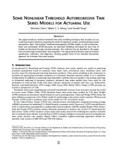
and economic forecasting containing two different data sets shown in Section 5.2. 5.1. Building Settlement Prediction. The prediction of future building settlement, especially for high-rising building, is a hot topic in Structural Health Monitoring. However, it is very difficult to develop good mathematical models and thus yield accurate predictions for building settlement, which is caused by the problems of small sample size (settlement observations are relatively few), nonstationary (the statistical properties of the measurement change over time), and nonlinearity (it is difficult to use mathematical prediction models with linear structure) [33]. The application illustrated in this section is the future settlement forecasting for Changchun branch’s business building of China Everbright Bank. The building has a steel structure form, with 28 floors above ground, and a base area of 2176 square meters. There are ten observation points marked 𝐾1, 𝐾2, . . . , 𝐾10. Observation settlement series 𝑥𝑡(𝑘) (𝑘 = 1, 2, . . . , 10, 𝑡 = 1, 2, . . . , 18), corresponding to each observation point 𝐾1, 𝐾2, . . . , 𝐾10, was got [34]. See Figure 1 for the data sets. It can be seen that the problems of small sample size, nonlinear, and nonstationary all exist. The last 3 settlement values are predicted based on the former 15 data. The GM(1,1) model, GM(1,1) rolling model, and AR model with linear interpolation [34] are adopted as reference methods for comparisons. Before AR model construction, the sample size of each data set is increased from 18 to 35 through linear interpolation; that is, a new (𝑘) (𝑘) )/2 is inserted between 𝑥𝑖(𝑘) and 𝑥𝑖+1 ,𝑖 = data (𝑥𝑖(𝑘) + 𝑥𝑖+1 1, 2, . . . , 17, 𝑘 = 1, 2, . . . , 10. And this is so called AR model with linear interpolation. To demonstrate the effectiveness and reasonability, the prediction results are analyzed by the index of average relative (𝑘) ̂𝑡(𝑘) | × 100/𝑥𝑡(𝑘) , percentage error ARPE = (1/10) ∑10 𝑘=1 |𝑥𝑡 − 𝑥 (𝑘) 𝑡 = 16, 17, 18, where 𝑥̂𝑡 is the prediction result corresponding to observation point 𝑘 = 1, 2, . . . , 10. The comparative results are listed in Table 6, which show that the most precise forecast is given by ARPRM, the following one is obtained by AR model with linear interpolation, and a considerably unreasonable accuracy is got by the GM(1,1) model and GM(1,1) rolling model. One problem worth noticing is that, in the AR model with linear interpolation processing procedure, the former 32 values of the interpolation series are utilized to conduct a 5-step-ahead prediction. And the forecasting result of the last 3 settlement values at 𝑡 = 16, 17, 18, which correspond to 𝑡∗ = 33, 35, 37 in the interpolated sequence,


7 2

0

−2

−4

K5 K3

K2

−6

K4

Settlement value (mm)

Settlement value (mm)

0 K1

K6

−2

K10

−4

K7 K9

−6

K8

−8 0

3

12

9

6

15

18

−8

0

3

6

9

12

15

18

t

t (a)

(b)

Figure 1: (a) Settlement sequence for observational point 𝐾1 to 𝐾5. (b) Settlement sequence for observational point 𝐾6 to 𝐾10.

Annual Chinese power load/(kW·h)

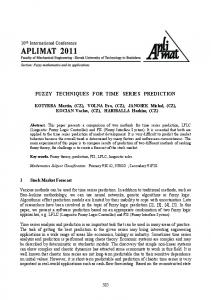
5.2. Economic Forecasting. In this section, our empirical study is also devoted to the comparison of our forecasting procedure with GM(1,1) model, GM(1,1) rolling model, and AR model with linear interpolation. The economic data sets include Chinese annual power load data [35] and Chinese annual gross domestic product (GDP) data [36] from 1987 to 2002, seen in Figures 2 and 3. We predict the latest two data with the former 14 for Chinese annual power load and GDP. The index of relative percentage error RPE = |𝑥𝑡 − 𝑥̂𝑡 | × 100/𝑥𝑡 is used to demonstrate the accuracy. The comparative results for each economic data set are listed in Tables 7 and 8. Table 7 shows that ARPRM derives the best prediction accuracy, and GM(1,1) model and GM(1,1) rolling model also give good forecast results for the Chinese annual power load forecast. Although AR model with linear interpolation provides the worst prediction, its accuracy is still acceptable. A similar conclusion with Section 5.1 can be obtained for the Chinese annual GDP prediction results. Based on the empirical study discussed above, it can be concluded that prediction accuracy of ARPRM and AR model with linear interpolation method is relatively stable. Precision of GM(1,1) model and GM(1,1) rolling model is considerably good when data set show an exponential trend, such as Chinese annual power load. Otherwise, the prediction accuracy of GM(1,1) model and GM(1,1) rolling model cannot be satisfied when nonexponential data exist. In addition, GM(1,1) rolling approach derives a better prediction precise compared with GM(1,1) model, and this is the superiority of the rolling mechanism.

16000 14000 12000 10000 8000 6000 4000 1986

1988

1990

1992

1994

1996

1998

2000

2002

Time (year)

Figure 2: Chinese annual power load data.

Annual Chinese GDP/Billion RMB

can be derived. In can be seen that the 32nd value, obtained ∗(𝑘) (𝑘) (𝑘) = (𝑥15 + 𝑥16 )/2, contains the information interpolation 𝑥32 (𝑘) of 𝑥16 that we want to predict. Actually, this interpolation ∗(𝑘) cannot be utilized in the forecasting. value 𝑥32

10000

8000

6000

4000

2000 1986 1988 1990 1992 1994 1996 Time (year)

1998 2000 2002

Figure 3: Chinese annual GDP.

8

Mathematical Problems in Engineering Table 6: ARPE of the prediction results (%).

ARPE

ARPRM

GM(1,1) model

GM(1,1) rolling model

AR model with linear interpolation

𝑡 = 16 𝑡 = 17 𝑡 = 18

3.87 7.46 12.15

30.96 48.75 71.23

30.96 44.80 65.98

3.69 11.66 18.17

Table 7: ARPE of the Chinese annual power load prediction results (%). ARPE

ARPRM

GM(1,1) model



𝑡 = 15 𝑡 = 16

3.08 0.14

0.68 4.17

0.68 4.42

0.08 7.37

Table 8: ARPE of the Chinese annual GDP prediction results (%). ARPE

ARPRM

GM(1,1) model



𝑡 = 15 𝑡 = 16

5.77 7.61

23.22 31.53

23.22 32.50

1.83 10.18

6. Conclusions This study presents a novel approach to settle the small sample time series prediction problem in the presence of unstable. One should construct an ARPRM model independently based on the metabolism sample in every prediction step. In other words, the model order and parameters are modified in each new forecasting step. This modification is much helpful to improve the prediction accuracy in small sample circumstance. We should note that the autoregressive in this study, which can model nonstationary sequences, is different from the AR method in the literature, which has to satisfy the stationarity requirement. Simulation study first conducts a general verification, then monitors the performance of the ARPRM method while varying the sample size and nonlinearity dynamic mechanism, and finally checks whether the reasonability depends on the variance of the innovation. We also performed statistical analysis to demonstrate the significance of the observed trends. Results show that factors including sample size, nonlinearity dynamic mechanism, significance of trends, and innovation variance do impacts on the performance of the proposed methodology. Specifically, we found that the nonlinearity plays a much more important role in forecasting performance than trend significance. For the same simulation model, precision will be enhanced while increasing sample size or reducing the innovation variance. Meanwhile, the established approach will illustrate a better property for the dynamic mechanisms that show a stronger linearity. Comparing the results in simulation study in Section 4, it can be seen that innovation variance (the uncertainty or randomness) has a greater effect on the performance. Empirical applications with building settlement prediction and economic forecasting are also included. The results show that the proposed method outperforms the Grey prediction model GM(1,1) and GM(1,1) rolling model, and AR

model with linear interpolation, and also illustrate a promise for future applications in small sample time series prediction.

Conflict of Interests The authors declare that there is no conflict of interest regarding the publication of this paper.

Acknowledgments The authors are grateful to the anonymous reviewers and the editor for their critical and constructive comments on this paper. This study was cosupported by the National Natural Science Foundation of China (Grant no. 11202011), National Basic Research Program of China (973 Program) (Grant no. 2012CB720000), and Fundamental Research Funds for the Central Universities (Grant no. YWK13HK11).

References [1] F. Busetti and J. Marcucci, “Comparing forecast accuracy: a Monte Carlo investigation,” International Journal of Forecasting, vol. 29, no. 1, pp. 13–27, 2013. [2] W. K. Wong, M. Xia, and W. C. Chu, “Adaptive neural network model for time-series forecasting,” European Journal of Operational Research, vol. 207, no. 2, pp. 807–816, 2010. [3] S. Makridakis, S. C. Wheelwright, and R. J. Hyndman, Forecasting-Methods and Applications, John Wiley & Sons, New York, NY, USA, 3rd edition, 1998. [4] J. D. Farmer and J. J. Sidorowich, “Predicting chaotic time series,” Physical Review Letters, vol. 59, no. 8, pp. 845–848, 1987. [5] Y.-H. Lin and P.-C. Lee, “Novel high-precision grey forecasting model,” Automation in Construction, vol. 16, no. 6, pp. 771–777, 2007. [6] P. Pinson, “Very-short-term probabilistic forecasting of wind power with generalized logit-normal distributions,” Journal of


[7]

[8] [9]

[10]

[11]

[12]

[13]

[14]

[15]

[16]

[17]

[18] [19]

[20]

[21]

[22] [23]

[24]

the Royal Statistical Society C: Applied Statistics, vol. 61, no. 4, pp. 555–576, 2012. P. G. Zhang, “Time series forecasting using a hybrid ARIMA and neural network model,” Neurocomputing, vol. 50, pp. 159– 175, 2003. J. D. Hamilton, Time Series Analysis, Princeton University Press, Princeton, NJ, USA, 1994. S. Liu, E. A. Maharaj, and B. Inder, “Polarization of forecast densities: a new approach to time series classification,” Computational Statistics & Data Analysis, vol. 70, pp. 345–361, 2014. A. Gelman and J. Hill, Data Analysis Using Regression and Multilevel/Hierarchical Models, Cambridge University Press, Cambridge, UK, 2007. M. Hofmann, C. Gatu, and E. J. Kontoghiorghes, “Efficient algorithms for computing the best subset regression models for large-scale problems,” Computational Statistics & Data Analysis, vol. 52, no. 1, pp. 16–29, 2007. R. Ghazali, A. Jaafar Hussain, N. Mohd Nawi, and B. Mohamad, “Non-stationary and stationary prediction of financial time series using dynamic ridge polynomial neural network,” Neurocomputing, vol. 72, no. 10–12, pp. 2359–2367, 2009. E. Kayacan, B. Ulutas, and O. Kaynak, “Grey system theorybased models in time series prediction,” Expert Systems with Applications, vol. 37, no. 2, pp. 1784–1789, 2010. G. Rubio, H. Pomares, I. Rojas, and L. J. Herrera, “A heuristic method for parameter selection in LS-SVM: application to time series prediction,” International Journal of Forecasting, vol. 27, no. 3, pp. 725–739, 2011. G. Huerta and M. West, “Priors and component structures in autoregressive time series models,” Journal of the Royal Statistical Society B: Statistical Methodology, vol. 61, no. 4, pp. 881–899, 1999. G. Huerta and M. West, “Bayesian inference on periodicities and component spectral structure in time series,” Journal of Time Series Analysis, vol. 20, no. 4, pp. 401–416, 1999. E. J. McCoy and D. A. Stephens, “Bayesian time series analysis of periodic behaviour and spectral structure,” International Journal of Forecasting, vol. 20, no. 4, pp. 713–730, 2004. M. A. Sharaf, D. L. Illman, and B. R. Kowalski, Chemometrics, John Wiley & Sons, New York, NY, USA, 1986. W. Zheng and A. Tropsha, “Novel variable selection quantitative structure-property relationship approach based on the Knearest-neighbor principle,” Journal of Chemical Information and Computer Sciences, vol. 40, no. 1, pp. 185–194, 2000. A. Porta, G. Baselli, S. Guzzetti, M. Pagani, A. Malliani, and S. Cerutti, “Prediction of short cardiovascular variability signals based on conditional distribution,” IEEE Transactions on Biomedical Engineering, vol. 47, no. 12, pp. 1555–1564, 2000. J. H. Stock and M. W. Watson, “A comparison of linear and nonlinear univariate models for forecasting macroeconomic time series,” in Cointegration, Causality and Forecasting, R. F. Engle and H. White, Eds., Oxford University Press, Oxford, UK, 1999. M. P. Clements and D. F. Hendry, Forecasting Economic Time Series, Cambridge University Press, Cambridge, UK, 1998. J. Bai and P. Perron, “Estimating and testing linear models with multiple structural changes,” Econometrica, vol. 66, no. 1, pp. 47– 78, 1998. J. Bai and P. Perron, “Computation and analysis of multiple structural change models,” Journal of Applied Econometrics, vol. 18, no. 1, pp. 1–22, 2003.

9 [25] K. L. Wen, Grey Systems, Yang’s Scientific Press, Tucson, Ariz, USA, 2004. [26] D. Akay and M. Atak, “Grey prediction with rolling mechanism for electricity demand forecasting of Turkey,” Energy, vol. 32, no. 9, pp. 1670–1675, 2007. [27] W. W. S. Wei, Time Series Analysis, Addison Wesley, Redwood City, Calif, USA, 2nd edition, 2006. [28] P. Sørensen, N. A. Cutululis, A. Vigueras-Rodr´ıguez et al., “Power fluctuations from large wind farms,” IEEE Transactions on Power Systems, vol. 22, no. 3, pp. 958–965, 2007. [29] V. Akhmatov, “Influence of wind direction on intense power fluctuations in large ofshore windfamrs in the North Sea,” Wind Engineering, vol. 31, no. 1, pp. 59–64, 2007. [30] M. di Rienzo, G. Parati, G. Mancia, A. Pedotti, and P. Castiglioni, “Investigating baroreflex control of circulation using signal processing techniques,” Engineering in Medicine and Biology Magazine, vol. 16, no. 5, pp. 86–95, 1997. [31] A. Porta, P. Castiglioni, M. D. Rienzo et al., “Information domain analysis of the spontaneous baroreflex during pharmacological challenges,” Autonomic Neuroscience: Basic and Clinical, vol. 178, pp. 67–75, 2013. [32] H. Akaike, “A new look at the statistical model identification,” IEEE Transactions on Automatic Control, vol. 19, pp. 716–723, 1974, System identification and time-series analysis. [33] H. Sohn, C. R. Farrar, F. M. Hemez et al., “A review of structural health monitoring literature: 1996–2001,” Tech. Rep. LA-13976MS, Los Alamos National Laboratory, Los Alamos, NM, USA, 2004. [34] X. Lin, Application of Time Series Analysis to the Buildings Deformation Monitor, Ji Lin Univercity, Changchun, China, 2005. [35] China Electric Power Committee, China Electric Power Yearbook 2003, China Electric Power Publishing House, Beijing, China, 2003. [36] National Bureau of Statistics of China, China Statistical Yearbook 2003, China Statistics Press, Beijing, China, 2003.

Advances in

Operations Research Hindawi Publishing Corporation http://www.hindawi.com

Volume 2014

Advances in

Decision Sciences Hindawi Publishing Corporation http://www.hindawi.com

Volume 2014

Journal of

Applied Mathematics

Algebra

Hindawi Publishing Corporation http://www.hindawi.com


Volume 2014

Journal of

Probability and Statistics Volume 2014

The Scientific World Journal Hindawi Publishing Corporation http://www.hindawi.com


Volume 2014

International Journal of

Differential Equations Hindawi Publishing Corporation http://www.hindawi.com

Volume 2014

Volume 2014

Submit your manuscripts at http://www.hindawi.com International Journal of

Advances in

Combinatorics Hindawi Publishing Corporation http://www.hindawi.com

Mathematical Physics Hindawi Publishing Corporation http://www.hindawi.com

Volume 2014

Journal of

Complex Analysis Hindawi Publishing Corporation http://www.hindawi.com

Volume 2014

International Journal of Mathematics and Mathematical Sciences


Journal of

Mathematics Hindawi Publishing Corporation http://www.hindawi.com

Volume 2014


Volume 2014

Volume 2014


Volume 2014

Discrete Mathematics

Journal of

Volume 2014


Discrete Dynamics in Nature and Society

Journal of

Function Spaces Hindawi Publishing Corporation http://www.hindawi.com

Abstract and Applied Analysis

Volume 2014


Volume 2014


Volume 2014

International Journal of

Journal of

Stochastic Analysis

Optimization



Volume 2014

Volume 2014