AVA: Automated Interpretation of Dynamically Detected Anomalies Anton Babenko
Leonardo Mariani
Fabrizio Pastore
University of Milano Bicocca viale Sarca, 336 20126 - Milano, Italy
University of Milano Bicocca viale Sarca, 336 20126 - Milano, Italy
University of Milano Bicocca viale Sarca, 336 20126 - Milano, Italy
[email protected]
[email protected]
[email protected]
ABSTRACT
1.
Dynamic analysis techniques have been extensively adopted to discover causes of observed failures. In particular, anomaly detection techniques can infer behavioral models from observed legal executions and compare failing executions with the inferred models to automatically identify the likely anomalous events that caused observed failures. Unfortunately the output of these techniques is limited to a set of independent suspicious anomalous events that does not capture the structure and the rationale of the differences between the correct and the failing executions. Thus, testers spend a relevant amount of time and effort to investigate executions and interpret these differences, reducing effectiveness of anomaly detection techniques. In this paper, we present Automata Violations Analyzer (AVA), a technique to automatically produce candidate interpretations of detected failures from anomalies identified by anomaly detection techniques. Interpretations capture the rationale of the differences between legal and failing executions with user understandable patterns that simplify identification of failure causes. The empirical validation with synthetic cases and third-party systems shows that AVA produces useful interpretations.
Anomaly detection techniques can support testers by automatically providing information about the unexpected events that have been observed in failing executions [13, 19, 11, 14, 27, 20, 26]. Focusing failure investigation on the information provided by these techniques often facilitates the understanding of the possible failure causes and simplify the localization of faults. Anomaly detection techniques usually work in two steps. In the first step, they generate a model of the legal behavior of a target system by tracing successful executions at testingtime, and then synthesizing models from the collected traces. In the second step, they compare the set of events detected during failing executions with the generated models to identify the anomalous events that will be presented to testers.
INTRODUCTION
0
1
2
3
Figure 1: A sample FSA used for anomaly detection.
Categories and Subject Descriptors D.2.5 [Software Engineering]: Testing and Debugging— Debugging aids, Tracing, Monitors; D.2.4 [Software Engineering]: Software/Program Verification—Validation
General Terms Verification
Keywords Anomaly detection, Dynamic Analysis
Permission to make digital or hard copies of all or part of this work for personal or classroom use is granted without fee provided that copies are not made or distributed for profit or commercial advantage and that copies bear this notice and the full citation on the first page. To copy otherwise, to republish, to post on servers or to redistribute to lists, requires prior specific permission and/or a fee. ISSTA’09, July 19–23, 2009, Chicago, Illinois, USA. Copyright 2009 ACM 978-1-60558-338-9/09/07 ...$5.00.
Even if data about anomalous events can be useful, in many cases investigating and interpreting such data can be extremely time consuming. Consider the case of a technique that derives the Finite State Automaton (FSA) shown in Figure 1 to detect anomalies. The FSA specifies that the target system usually generates the following sequence of events during correct executions: a file is opened, data are written in the file, the file is closed and finally sent through the network. In case a fault causes the file to not being closed, the anomaly detection technique would compare the sequence of events File.open, File.write, . . . , File.write, sendFile, observed in the failing execution, with the model. The result would be that the event sendFile is not accepted by the model, and sendFile would be presented to testers as anomalous event. Testers may erroneously think that something is wrong in the functionality for sending files, and they would start their investigation from components and libraries for managing file transfer. Once this investigation failed, testers would probably consider other possibilities and identify the right cause of the failure. This simple investigation may require several minutes or even hours to be completed. In case many anomalous events or complex re-arrangement of events are detected in failing
executions, e.g., interleaved events, postponed events, etc., the effort required to interpret and investigate anomalous events can be extremely high, with a dramatic loss of costeffectiveness of the technology. In this paper, we present a technique, called Automata Violation Analyzer (AVA), that automatically analyzes anomalous events identified by dynamic analysis techniques that infer FSA. The technique produces multiple interpretations of the detected anomalies, prioritizes them according to likelihood to explain differences between correct and failing executions, and presents the final result to testers. We focus on FSA because they are commonly used to represent component behaviors and interaction protocols, can be inferred by many algorithms [3, 1, 14], and are used by several anomaly detection techniques [1, 13, 20, 26, 14]. We integrated AVA with Log File Analysis (LFA), a technique developed for automated analysis of log files [13]. We experienced the integrated solution with both synthetic cases and third-party systems. Synthetic cases are used to simulate the different kinds of anomalies that can be experienced in software systems. Third-party systems are used to validate our solution with large applications. Empirical results show that AVA correctly presents a suitable interpretation of failure causes within the fifth interpretation of the ranking. The paper is organized as follow. Section 2 summarizes the main steps of the AVA technique. Section 3 describes LFA. Section 4 presents strategies to identify basic interpretations from detected anomalies. Section 5 presents strategies to identify composite interpretations from detected anomalies. Section 6 describes the prioritization criterion used to order interpretations. Section 7 presents empirical results obtained with synthetic cases and third-party systems. Section 8 discusses related work. Finally, Section 9 concludes the work.
2.
AVA
AVA can automatically provide an effective interpretation to a set of anomalies that has been detected by an anomaly detection technique that uses inferred FSAs to represent the expected behavior of software systems. Thus, the complete solution is the result of the integration of two main techniques: an anomaly detection technique and AVA. The anomaly detection technique is responsible for monitoring a target system, deriving a model of the expected behavior, and identifying anomalous events in failing executions. AVA is responsible for interpreting data, identifying candidate explanations to observed problems and prioritizing the results. In the next section, we shortly describe LFA, the technique for anomaly detection that we integrated in our solution [13]. Here we summarize the three main phases of AVA: identify basic interpretations, identify composite interpretations, and prioritize interpretations. Identify basic interpretations consists of analyzing both anomalies and inferred models used to identify such anomalies to generate a more relevant, even if simple, interpretation about the unexpected events. For instance, the anomalous sendFile event identified with the model in Figure 1 generated by a failing execution that did not close the file before sending it through the network can be more relevantly explained as a missing File.close event. Identify composite interpretations consists of analyzing and combining the available set of simple interpretations
to identify richer interpretations of failing executions. For instance, if both a missing event and the addition in the future of the same missing event are identified as simple interpretations, a postponed event represents a more precise interpretations of the failing execution. Prioritize interpretations consists of ordering basic and composite interpretations according to their likelihood to effectively explain differences between correct and failing executions. Ordering interpretations is useful to start the investigation of failure causes from good interpretations, and avoid the investigation of interpretations with little relevance.
3.
LOG FILE ANALYSIS
LFA is a dynamic analysis technique that automatically identifies anomalous events in log files recorded during failing executions [13]. LFA is based on three main phases: monitoring, model generation and failure analysis. Monitoring consists of collecting traces of correct executions from target systems. A trace is a sequence of events annotated with attribute values. Monitoring takes typically place at testing time, when it is simple to distinguish failing and correct executions. Model generation is the most complex phase of the technique and consists of generating a FSA that summarizes and generalizes all the collected traces. LFA initially processes trace files to automatically identify event names and attribute values. This operation is executed because LFA does not require the complete knowledge of the log format in advance, but heuristically infers the format. It is sufficient that event names and their attribute values are recorded in a text file separated by a known character. In other words it is only known when an event entry (event name followed by attribute values) begins and ends. Thank to this feature, it is extremely simple to adapt LFA to different log formats. Since attribute values often capture information that is specific to a given execution, but with little relevance when compared with other executions, such as the case of process identifiers, LFA pre-processes attribute values to extract more general and reusable information than concrete attribute values. In particular, LFA eliminates attribute values and modifies event names to incorporate information about the regularity of the distribution of those values across events. The rewriting of the event names is based on the identification of recurrent definition-use patterns across attribute values. For instance, if an analyzed log file includes a trace like start p1210, start p1084, stop p1210, stop p1084 where start and stop are event names and p1210 and p1084 are attribute values, LFA rewrites this trace as start_A, start_B, stop_A, stop_B where only event names occur1 . The rewritten trace has the benefit to include information about the expected attribute values, i.e., processes are started and stopped in the same order, even if it only includes event names without attribute values. Thus, the rewritten traces can be used to infer mod1 this example presents the simplest rewriting strategy available in LFA.
els capable to reveal failures that depend on attribute values. Let us consider the sequence of events start p4567, start p1234, stop p1234, stop p4567 which starts and stops processes with a different order than the previous trace. Let us also suppose that a failure occurs when this example sequence is observed. According to the previous strategy, the sequence would be rewritten as start_A, start_B, stop_B, stop_A. If we compare the two rewritten sequences, we discover that the first two events match (start_A and start_B), while the third and the fourth differ (stop_B and stop_A). This difference successfully indicates that processes are terminated with an unexpected order. Simply ignoring attribute values and only matching event names would not have revealed such difference. LFA includes mechanisms to automatically and heuristically identify likely related attributes, and independently rewrite different groups of homogeneous attributes. For instance, attribute values that indicate IP addresses and values that indicate meters would be rewritten and verified independently. Thus avoiding comparisons of unrelated attributes. LFA can derive models at different levels of granularity. For instance, it is possible to derive a unique model that specifies the behavior of the whole system, or to derive one model for each component that is monitored, to better focus on the events generated by each unit. More details about these mechanisms, further technicalities to handle multiple attribute values associated with events, and to increase robustness with respect to noise and incidental values can be found in [13]. For the purpose of the work presented in this paper, it is sufficient to know that LFA considers attribute values in the analysis even if it infers plain FSA. The model generation phase is completed by using kBehavior to infer the final FSA that summarizes and generalizes the rewritten traces provided as input [14]. When a failure is investigated, LFA reads the trace recorded during the failing execution and uses this trace to extend the model that represents correct executions. Several techniques simply compare a trace with a model to indicate the first event that is not accepted by the model. This strategy hinders visibility of many anomalies that may be located after the first one. Thus a little noise can heavily reduce effectiveness of the technique. To overcome this issue, LFA does not check whether the model accepts the trace or not, but extends the model considering the trace as an extra input (kBehavior provides the capability to incrementally extend FSA by processing additional traces). The extended model will generate both the language generated by the original model and the trace that corresponds to the failing execution. All the changes introduced during the extension are interpreted by LFA as unexpected event sequences that occurred in the failing execution. According to experiments reported in [13], LFA can identify a small set of anomalous events (between 0.01% and 28.57% of the total number of recorded events) with an average precision of 0.67 when suitable configurations are selected by testers. Even if a precision of 0.67 indicates that a relevant percentage of the anomalies presented to testers are in effect related to failures, interpreting these data can still be hard and time consuming.
4.
BASIC INTERPRETATIONS
The first operation executed by AVA consists of automatically identifying basic interpretations, i.e., interpretations of the anomalies detected in a failing execution specified according to a catalog of user-understandable basic anomaly patterns. Formally, an interpretation is a triple , where anomaly pattern is the name of an anomaly pattern; confidence value is a confidence value in the range 0 to 1 that specifies how much the anomaly pattern well describes anomalies observed in the failing execution; and extra info specifies additional information that easy the understanding of the interpretation. Basic interpretations are derived by locally analyzing single anomalies (the way we implemented locality is presented in Section 4.1). An example basic interpretation is . The first item delete specifies that the interpretation refers to the delete anomaly pattern. The confidence value 1 indicates perfect confidence on the interpretation, thus the only difference between the expected behavior and the observed behavior consists of deleted events. The last element of the triple specifies that only the event F ile.close has been deleted, and presents both the observed event sequence and the expected correct sequence that is closest to the observed one. Section 4.2 describes how we compute confidence values. The identification of basic interpretations is based on two steps: (1) define scope and expected behaviors, and (2) align and score basic anomaly patters. Define scope and identify expected behaviors consists of identifying the legal behaviors accepted by the inferred FSA that are close to the anomaly under analysis. Align and score basic patterns consists of executing a customized string alignment algorithm to compare possible behaviors with the failing execution and measure how well each basic anomaly patterns describes the observed anomaly.
4.1
Define scope and expected behaviors
AVA analyzes each anomaly by comparing the expected event sequences and the observed event sequence. To reduce the size of the problem and concentrate the analysis on the target anomaly, the comparison is restricted to the expected and observed events that are close to the place where the anomaly has been detected. The exact scope of the analysis depends on the kind of analyzed anomaly. Since LFA represents anomalies as extensions of FSAs, the kind of anomalies to be analyzed can be classified according to the type of extension introduced by LFA. In particular, LFA can extend a model in three possible ways: adding a branch, adding a tail, and adding a final state.
Branch extension A branch extension consists of extending a FSA with the addition of a new branch, as shown in Figure 2. A new branch has an extension start point and an extension end point. The extension start point is the state of the FSA augmented with a new outgoing transition. The extension end point is the state of the FSA augmented with a new incoming transition. We can have two kinds of branch extensions: branches
pointing to the future and branches pointing to the past. We have a branch pointing to the future when the extension end point is reachable from the extension start point. This extension indicates that a new behavior has been observed instead of an expected behavior. We have a branch pointing to the past when the extension end point is not reachable from the extension start point in the original FSA. This extension indicates that an expected behavior has been unexpectedly observed multiple times. extension start point
a
...
extension end point
b
newB
a
newA
b doC
doA
0
doB
doC
2
1
3
...
doF
doD
4
doG
sequences obtained by sequences of max length 1: covering a state at most twice: doB doC doD
5
sequences of max length 1: doF doG
set of local expected behaviors considered in the analysis of an anomaly resulted in a branch extension: seq1) doB doC doD doF seq2) doB doC doD doG
...
sequence observed in the failing execution: doA doB newA newB doC doF … subsequence selected for the local analysis: doB newA newB doC doF
0
1
sequences of max length k1
... sequences obtained by covering a state at most twice
8
9 sequences of max length k2
Figure 3: An example set of behaviors considered in the analysis of a branch extension pointing to the future
set of local expected behaviors considered in the analysis of an anomaly resulted in a branch extension
length of the branch = l extension end point
Figure 2: A branch extension pointing to the future We define the scope of the local analysis depending on the kind of branch that has been added. In the case of a branch pointing to the future, we consider behaviors immediately preceding the anomaly, i.e., immediately preceding the extension start point, alternative to the anomaly, i.e., between the extension start and end points, and immediately following the anomaly, i.e., immediately following the extension end point. In particular, we consider the event sequences that can be obtained by concatenating the sequences of maximum length k1 that can be generated before the extension start point, the sequences of events that can be generated between the extension start point and the extension end point by traversing each state at most twice, and the sequences of events of maximum length k2 that can be generated after the extension end point. Parameters k1 and k2 are integer values defined by testers to tune the scope of the local analysis. We extend the boundaries of the local analysis outside extension start and end points because some interpretations can depend on events located before or after the extension points, e.g., postponed events and added events. Figure 2 visually shows the set of events that are considered in the local analysis of a branch pointing to the future. The subsequence of the events observed in the failing execution to be compared with the expected behaviors is selected with an analogous strategy, i.e., we consider the k1 events before the first event in the branch pointing to the future, the events in the branch pointing to the future, and the k2 events after the last event in the branch pointing to the future. Figure 3 shows the expected and observed sequences that are considered for the analysis with an example FSA and k1 = k2 = 1. In the case of a branch pointing to the past, we consider behaviors immediately preceding the anomaly, i.e., immediately preceding the extension start point, and immediately following the anomaly, i.e., immediately following the ex-
a
...
extension start point
b
... 0
1
... sequences of max length k1
8
9 sequences of max length (l+k2)
set of local expected behaviors considered in the analysis of an anomaly resulted in a branch extension
Figure 4: A branch extension pointing to the past
tension start point. In particular, we consider the event sequences that can be obtained by concatenating the sequences of maximum length k1 that can be generated before the extension start point and the sequences of events of maximum length k2 +l that can be generated after the extension start point, where l is the length of the branch pointing to the past. We take into account the length l of the branch generated by the anomaly to consider expected sequences with the same length than the subsequence considered for the failing execution. Figure 4 visually shows the set of events that are considered in the local analysis of a branch pointing to the past. We adopt an analogous strategy to select the subsequence of the events observed in the failing execution to be compared with the expected behaviors. In this case we consider the k1 events before the first event in the branch pointing to the past, the l events in the branch and the k2 events after the last event in the branch. Figure 5 shows the expected and observed sequences that are considered for the analysis with an example FSA and k1 = k2 = 2.
doF
newB doA 0
doB
b newA
doC 2
1
a
pected and observed sequences that are considered for the analysis with an example FSA and k1 = 2.
3
4
sequences of max length 2
doH
doF
doD
5
doG
doD
doL 6
7
sequences of max length (2+3=5)
newA
set of local expected behaviors considered in the analysis of an anomaly resulted in a branch extension: seq1) doC doD doF doH doL seq2) doC doD doG doH doL
doB
a
b
doC
doD
doE
doA
2
1
0
sequence observed in the failing execution: doA doB doC doD newA doF newB doC doD doG... subsequence selected for the local analysis: doC doD newA doF newB doC doD
3
sequences of max length 2: doA doB
Figure 5: An example set of behaviors considered in the analysis of a branch extension pointing to the past
4
...
sequences of max length 2: doC doD
set of local expected behaviors considered in the analysis of an anomaly resulted in a tail extension: seq1) doA doB doC doD
length of the tail = l sequence observed in the failing execution: doA doB newA doD subsequence selected for the local analysis: doA doB newA doD
extension start point
a
...
b
Figure 7: An example set of behaviors considered in the analysis of a tail extension
... 0
1
sequences of max length k1
2
Final state extension
sequences of max length l
extension point
... set of local expected behaviors considered in the analysis of an anomaly resulted in a tail extension
0
1
2
Figure 6: Tail extension no local expected behaviors considered in the analysis
Tail extension A tail extension consists of extending a FSA with the addition of a new tail, as shown in Figure 6. A new tail has an extension start point and a final state at the end of the tail. The extension start point is the state of the FSA which is augmented with a new outgoing transition. We define the scope of the analysis as the set of behaviors immediately preceding the anomaly, i.e., immediately preceding the extension start point, and immediately following the anomaly, i.e., immediately following the extension start point. In particular, we consider the event sequences that can be obtained by concatenating the sequences of maximum length k1 that can be generated before the extension start point with the sequences of events of maximum length l that can be generated after the extension start point, where l is the length of the tail (this choice guarantees the analysis of expected and failing sequences of the same length). Figure 6 visually shows the set of events that are considered in the local analysis of a tail. The subsequence of the observed behavior to be compared with expected behaviors is selected with an analogous strategy, i.e., we consider the k1 events before the first event in the tail and the l events in the tail. Figure 7 shows the ex-
Figure 8: Final state extension A final state extension consists of extending a FSA by replacing a regular state with a final state, as shown in Figure 8. A final state extension has an extension point which is the replaced state. This kind of extension is a special case because there are no unexpected events: the execution simply terminated at an anticipated time. In this case, local analysis is not needed because the anticipated interruption of the execution is identified with perfect confidence.
4.2
Align and score basic patterns
In the previous step, we selected the expected behaviors to be considered for local analysis. In this step, we compare each expected behavior with the sequence observed in the failing execution to interpret differences. These differences will be presented to testers as likely failure causes. To evaluate the relevance of a given interpretation, we compute its confidence values as the distance between each pair . A distance
is a real value in the range 0..1 that indicates how well a given interpretation fits the case under analysis. Traces collected during failing executions often include noise, i.e., events that are not accepted by the model and are not directly related to the investigated failure. Since LFA extends a FSA with a new trace by matching subsequences with sub-automata, and adding the extra states and transitions necessary to accept the whole trace, presence of noisy events can modify the sequences in the added branches or even cause the addition of new branches. To be applicable to large and complex cases, the strategy to recognize anomaly patterns must also work when extensions include noise. To this end, we use a string alignment algorithm that compares the local expected behavior with the local anomalous behavior and finds a proper fitting of events, despite presence of noisy data. We run our string alignment algorithm with different configurations corresponding to the kind of basic interpretation that is investigated. Each possible alignment of the two analyzed event sequences is associated with a score that indicates how much the two strings are close according to the selected configuration. For example, an observed and an expected sequence that only differs for deleted events will be extremely close according to the delete interpretation. The string alignment algorithm that we use is a modified version of the Needleman-Wunsch global alignment algorithm [17]. Our modified version can be configured to evaluate the differences between two aligned strings according to different weights. Depending on the alignment, we can have four results when comparing two aligned symbols: match, mismatch, deleteGap, and addGap. Figure 9 shows these cases. We have a match when there is the same symbol at the same position. We have a mismatch when there are two different symbols at the same position. We have a deleteGap when there is a symbol in the expected sequence and a gap in the observed sequence. We have an addGap when there is a gap in the expected sequence and a symbol in the observed sequence. Gaps are automatically introduced by the alignment algorithm to find the best correspondence between the two strings under analysis. We modified the alignment algorithm to support a different evaluation for the deleteGap and addGap. The original version of the algorithm cannot distinguish between these gaps. We modified the algorithm because gaps have not the same semantics in our domain, e.g., a deleteGap is a strongly favorable indication of deleted events, while an addGap is against this same interpretation.
The final score assigned to each possible alignment is computed by summing the weights associated with each symbol in the aligned sequence and then normalizing in the range 0..1 by dividing for the number of places (a place can be a symbol or a gap) in the aligned sequences. This score indicates the confidence value of the interpretation. We look for basic interpretations by defining configurations, i.e., sets of weights assigned to the possible result of symbol comparison, that positively evaluate matchings and differences that are consistent with the investigated interpretation, and negatively evaluate differences that are not consistent with the investigated interpretation. We defined four basic interpretations: delete, insert, replace and final state. In the following, we present the configuration of each basic interpretation, and we show with an example how each configuration is evaluated. It is worth to mention that interpretations are decorated with extra information that specifies the expected sequence that is closest to the anomalous sequence and the start state of the anomalous behavior.
Delete A delete interpretation is associated with the following weights: match = +1 mismatch = −1 deleteGap = +1 addGap = −1 Since we are analyzing an anomaly, it is not possible that all events match, thus the maximum evaluation is obtained when we have matches and some deleted events. Eventual noise represented by the presence of addGap and mismatch decreases the value of the interpretation. If we consider the sendFile example presented in the Introduction, the best alignment according to the configuration of a delete interpretation is shown in Figure 10. The example shows the case of a pure deleted event and the normalized value of the interpretation is in effect 44 = 1. Best alignment according to Delete: expected sequence: File.open File.write File.close sendFile observed sequence: File.open File.write sendFile
match +1
match +1
deleteGap +1
match +1
resulting sum = +4
Sequences to be aligned: expected sequence: doA doB doC doD doE observed sequence: doA doF doL doD doE
Figure 10: Example of a delete interpretation.
Possible alignment: expected sequence: doA doB doC doD doE observed sequence: doA doF doL doD doE
Insert An insert interpretation is associated with the following weights:
match
addGap mismatch
deleteGap
Figure 9: Example alignment.
match = +1 mismatch = −1 deleteGap = −1 addGap = +1
Since we are analyzing an anomaly, it is not possible that all events match, thus the maximum evaluation is obtained when we have matches and some added events. Eventual noise represented by the presence of deleteGap and mismatch decreases the value of the interpretation. Figure 11 shows an example interpretation of an insert. The example shows the case of a execution with mostly, but not purely, added events. In fact, the normalized value of the interpretation is 5 = 0.71. 7 Best alignment according to Insert: expected sequence: doA doB doC observed sequence: doA doB doExtra doExtra doExtra -
match +1
match +1
doD doD
addGap addGap addGap deleteGap +1 +1 -1 +1
match +1
resulting sum = +5
Figure 11: Example of an insert interpretation.
Replace A replace interpretation is associated with the following weights: match = +1 mismatch = +1 deleteGap = −1 addGap = −1 Since we are analyzing an anomaly, it is not possible that all events match, thus the maximum evaluation is obtained when we have matches and some mismatching events. Eventual noise represented by the presence of deleteGap and addGap decreases the value of the interpretation. Figure 12 shows an example interpretation of a replace. The example shows the case of an execution with mostly, but not purely, replaced events. In fact, the normalized value of the interpretation is 64 = 0.67. Best alignment according to Replace: expected sequence: doA doB doC observed sequence: doA doB doOther
match +1
match +1
doD doOther
mismatch mismatch +1 +1
doE -
doF doF
deleteGap -1
match +1
resulting sum = +4
Figure 12: Example of a replace interpretation.
Final state A final state interpretation does not require fine grained analysis to be discovered. In fact, every time a final state extension is detected, a final state interpretation with perfect confidence is generated. This interpretation indicates that the application terminated earlier than expected. Since with high probability a failing execution terminates differently than a regular execution, AVA frequently generates this interpretation. However, it exists at most one occurrence of this interpretation per analyzed failure. Thus,
this interpretation does not change readability of the output, while providing the useful information about the point where the application terminated its execution.
5.
COMPOSITE INTERPRETATIONS
Basic interpretations can be useful in many cases, however there exist further interesting interpretations that can be discovered by combining basic interpretations. We define a composite interpretation as an interpretation that is function of basic or composite interpretations. In the context of this work, we defined three composite interpretations: anticipation, posticipation and swap. In the following, we describe composite interpretations and show a few examples.
Anticipation An anticipation is the case of an event that occurs earlier than expected. We analyze anomalies to discover if an anticipation occurred in all the cases where we detect two basic interpretations I, D, where I is an insert or replacement interpretation, D is a delete or replacement interpretation, and I occurs before D in the trace recorded during the failing execution. To discover if an anticipation occurred, we define I.newEvents as the sequence of all the events in the observed sequence that are classified as added or mismatched, and D.removedEvents as the sequence that includes all the events in the expected sequence that are classified as deleted or mismatched. To discover if there are common symbols with same order between these two sequences (thus suggesting an anticipation), we align I.newEvents with D.removedEvents by using the following configuration: match = +1 mismatch = 0 deleteGap = 0 addGap = 0 The sequence alig of the symbols that match between I.newEvents and D.removedEvents after string alignment represents the events that have been anticipated. The sequence notAlig, which consists of the events that do not match after string alignment, includes events that are only added in the first interpretation, only deleted in the second interpretation or appear with the wrong order. If the number of aligned events is 0, we cannot have an anticipation. If we have at least 1 aligned event, we have a behavior that can be interpret as an anticipation, even if it may be associated with a low confidence value. We compute the confidence value of the anticipation by positively counting the events that are anticipated and the ones that match, and negatively counting the differences that do not contribute to the anticipation. In particular, if the interpretation I has I.m matches, I.n mismatches, I.a addGaps and I.d deleteGaps, and the interpretation D has D.m matches, D.n mismatches, D.a addGaps and D.d deleteGaps, and the sequence notAlig is further split into notAlig.g gaps and notAlig.n mismatches, the confidence value of the interpretation is computed as: 2∗]alig−2∗]notAlig.n−]notAlig.g+]I.m+]D.m−]I.d−]D.a length(I)+length(D)
where ] indicates the number of events in the sequence that follows.
Note that I.m, I.a, D.m and D.d do not appear explicitly in the formula for computing confidence value because events in these sequences have been used to generate the sequences alig and notAlig. Moreover, events in alig and notAlig.n are multiplied by a factor of 2 because two symbols (1 symbol per analyzed string) contribute to generate the case. Example insert interpretation: expected sequence: doA doB - doC observed sequence: doA doE doF doG doH doC Example delete interpretation: expected sequence: doI doL doF doG - doM observed sequence: doI - doN doM Sets specific to anticipation I.newEvents = doE doF doG doH D.removedEvents = doL doF doG Aligned sequences: doE doF doG doH doL doF doG alig = doF doG notAlig.n = doL notAlig.g = doH
A swap is the case of a sequence of events that are anticipated by replacing others that are posticipated. This interpretation can be easily discovered by combining the anticipation with the posticipation. In particular, if both such interpretations have been discovered for an observed trace, we also generate a swap interpretation with a confidence value given by the average value of the confidence values for the anticipation and the posticipation.
6.
General sets I.m = doA doC D.m = doI doM I.d = / D.a = doN
score =
Swap
2*2-2*1-1+2+2-0-1 6+6
= 0.33
confidence value =(0.33+1)/2=0.665 (normalized score)
Figure 13: Example of anticipation interpretation. Figure 13 shows an example application of the anticipation interpretation.
Posticipation The case of the posticipation is symmetric to the anticipation. A posticipation consists of events that occur later than expected. We analyze anomalies to discover if a posticipation occurred in all the cases where we detect two basic interpretations D, I, where D is a delete or replacement interpretation, I is an insert or replacement interpretation, and D occurs before I in the trace recorded during the failing execution. To discover if a posticipation occurred, we define D.removedEvents as the sequence that includes all the events in the expected sequence that are classified as deleted or mismatched, and I.newEvents as the sequence of all the events in the observed sequence that are classified as added or mismatched. To discover if there are common symbols with proper ordering between these two sequences (thus suggesting a posticipation), we align D.removedEvents and I.newEvents with the same configuration used for the anticipation. The sequence alig of the symbols that match after string alignment represents the events that have been posticipated. The sequence notAlig indicates events that are only deleted in the first interpretation, only added in the second interpretation or appear with the wrong order. If the number of aligned events is 0, we cannot have a posticipation. If we have at least 1 aligned event, we have a behavior that can be interpret as a posticipation, even if it may be associated with a low confidence value. We compute the confidence value of the posticipation by positively counting the events that are posticipated and the ones that match, and negatively counting the differences that do not contribute to the posticipation, resulting in the same formula used for the anticipation.
PRIORITIZE INTERPRETATIONS
Discovery of basic and composite interpretations ends with a list of possible interpretations that have a confidence value greater than 0. Since each anomaly can be compared with several possible expected behaviors, depending from the structure of the inferred FSA, and each pair < anomalous behavior, expected behavior > can have multiple explanations, the list of candidate interpretations can be large. For instance, if an inferred FSA specifies that the system under analysis can continue its execution in three possible ways just after the point where an anomaly has been detected, the anomalous behavior is compared with 3 possible expected behaviors. Considering that until now we have defined 4 possible types of basic interpretations, and 3 types of composites interpretations, the technique may produce tens of interpretations with confidence value greater than 0. To avoid having testers inspecting data with little interest, we rework the output produced by AVA in two steps: data aggregation and prioritization of the results. Data aggregation consists of building a unique representation of equivalent interpretations. The same interpretations for a same anomaly are represented as a single interpretation associated with the best confidence value. For instance, if a same anomaly has 3 possible explanations as an insert interpretation with confidence value 0.9, 0.7 and 0.2, we display insert only once with confidence value 0.9. If necessary, the tester can expand this information and see the other equivalent interpretations that have been hidden. This reduction is applied to both basic and composite interpretations. Finally, the overall set of resulting interpretations are globally ordered according to their confidence values. Since testers use AVA to look for explanations of observed failures, we present first explanations with high confidence values, thus clearly explaining differences between the expected behavior and the observed behavior, then the ones with low confidence value, which can be harder to read.
7.
EMPIRICAL VALIDATION
Interpretations are more descriptive than plain lists of suspicious events by construction. The empirical work aims at demonstrating that interpretations can describe real failure causes and that AVA can effectively discover them. In particular, we show that (1) AVA discovers interpretations that describe the differences between observed and expected behaviors, when these differences match our patterns, and (2) failure causes that can be described as AVA interpretations occur in real systems. To this end, we designed two empirical investigations. The first investigation focuses on a set of synthetic cases that have been automatically generated by our toolset. These cases cover the possible structure of the differences between expected and observed behaviors. We show that AVA effec-
Anomaly Type delete finalState insert replacement anticipation posticipation swap
Cases 36 36 36 36 180 180 180
ranking of the perfect 1