In particular: â We currently view average-case complexity as referring to the per- .... that some NP problems are not merely hard in the worst-case, but are rather.
Average Case Complexity, Revisited Oded Goldreich
Abstract. More than two decades elapsed since Levin set forth a theory of average-case complexity. In this survey we present the basic aspects of this theory as well as some of the main results regarding it. The current presentation deviates from our old “Notes on Levin’s Theory of Average-Case Complexity” (ECCC, TR97-058, 1997) in several aspects. In particular: – We currently view average-case complexity as referring to the performance on “average” (or rather typical) instances, and not as the average performance on random instances. (Thus, it may be more justified to refer to this theory by the name typical-case complexity, but we retain the name average-case for historical reasons.) – We include a treatment of search problems, and a presentation of the reduction of “NP with sampleable distributions” to “NP with P-computable distributions” (due to Impagliazzo and Levin, 31st FOCS, 1990). – We include Livne’s result (ECCC, TR06-122, 2006) by which all natural NPC-problems have average-case complete versions. This result seems to shed doubt on the association of P-computable distributions with natural distributions. Keywords: Average-Case Complexity.
This text has been revised based on [6, Sec. 10.2].
1
Introduction
In light of the apparent infeasibility of solving numerous useful computational problems, it is natural to ask whether these problems can be relaxed such that the relaxation is both useful and allows for feasible solving procedures. We stress two aspects about the foregoing question: on one hand, the relaxation should be sufficiently good for the intended applications; but, on the other hand, it should be significantly different from the original formulation of the problem so to escape the infeasibility of the latter. We note that whether a relaxation is adequate for an intended application depends on the application, and thus much of the material in this chapter is less robust (or generic) than the treatment of the non-relaxed computational problems. One commonly considered type of relaxation refers to the computational problems themselves; that is, for each problem instance we extend the set of admissible solutions. In the context of search problems this means settling for
102
solutions that have a value that is “sufficiently close” to the value of the optimal solution (with respect to some value function). Needless to say, the specific meaning of ‘sufficiently close’ is part of the definition of the relaxed problem. In the context of decision problems this means that for some instances both answers are considered valid; specifically, we shall consider promise problems in which the no-instances are “far” from the yes-instances in some adequate sense (which is part of the definition of the relaxed problem). In this survey, we consider a different type of relaxation. We do not relax the computational problems themselves, but rather the notion of solving them efficiently. Specifcally, this type of relaxation deviates from the requirement that the solver provides an adequate answer on each valid instance. Instead, the behavior of the solver is analyzed with respect to a predetermined input distribution (or a class of such distributions), and bad behavior may occur with negligible probability where the probability is taken over this input distribution. That is, we replace worst-case analysis by average-case (or rather typical-case) analysis. Needless to say, a major component in this approach is limiting the class of distributions in a way that, on one hand, allows for various types of natural distributions and, on the other hand, prevents the collapse of the corresponding notion of average-case hardness to the standard notion of worst-case hardness. 1.1
The basic mindframe of average-case complexity
The common approach of complexity theory is termed worst-case complexity, because it refers to the performance of potential algorithms on each legitimate instance (and hence to the performance on the worst possible instance). That is, computational problems were defined as referring to a set of instances and performance guarantees were required to hold for each instance in this set. In contrast, average-case complexity allows ignoring a negligible measure of the possible instances, where the identity of the ignored instances is determined by the analysis of potential solvers and not by the problem’s statement. A few comments are in place. Firstly, as just hinted, the standard statement of the worst-case complexity of a computational problem (especially one having a promise) may also ignores some instances (i.e., those considered inadmissible or violating the promise), but these instances are determined by the problem’s statement. In contrast, the inputs ignored in average-case complexity are not inadmissible in any inherent sense (and are certainly not identified as such by the problem’s statement). It is just that they are viewed as exceptional when claiming that a specific algorithm solve the problem; that is, these exceptional instances are determined by the analysis of that algorithm. Needless to say, these exceptional instances ought to be rare (i.e., occur with negligible probability). The last sentence raises a couple of issues. Most importantly, a distribution on the set of admissible instances has to be specified. In fact, we shall consider a new type of computational problems, each consisting of a standard computational problem coupled with a probability distribution on instances. Consequently, the question of which distributions should be considered in a theory of average-case
103
complexity arises. This question and numerous other definitional issues will be addressed in Section 2.1. Before proceeding, let us spell out the rather straightforward motivation to the study of the average-case complexity of computational problems: It is that, in real-life applications, one may be perfectly happy with an algorithm that solves the problem fast on almost all instances that arise in the relevant application. That is, one may be willing to tolerate error provided that it occurs with negligible probability, where the probability is taken over the distribution of instances encountered in the application. The study of average-case complexity is aimed at exploring the possible benefit of such a relaxation, distinguishing cases in which a benefit exists from cases in which it does not exist. A key aspect in such a study is a good modeling of the type of distributions (of instances) that are encountered in natural algorithmic applications. Let us consider the foregoing motivation from a slightly different perspective: The conjecture that P = 6 N P (or rather N P 6⊆ BPP) only asserts that intractability is a feature of some instances of some problems in N P. These intractable instances may be very rare and pathological. The theory of averagecase complexity addresses the question of whether intractability can also be a feature of “typical” instances (i.e., whether intractable instances may occur with noticeable probability with respect to some simple distributions). Needless to say, the meaningfulness of the latter question depends on restricting the class of distributions such that only simple (rather than pathological) distributions are allowed. We shall consider two such classes of distributions (see Section 2.1 and Section 3.2, respectively) and show that if intractability occurs with respect to the wider class then it occurs also with respect to the more restricted class (see Theorem 14). An average-case version of the P = 6 N P question. Indeed, a fundamental question that arises is whether every natural computational problem can be solved efficiently when restricting attention to typical instances? The conjecture that underlies this section is that, for a well-motivated choice of definitions, the answer is negative; that is, our conjecture is that the “distributional version” of NP is not contained in the average-case (or typical-case) version of P. This means that some NP problems are not merely hard in the worst-case, but are rather “typically hard” (i.e., hard on typical instances drawn from some simple distribution). This suggests that hard instances may occur in natural algorithmic applications (and not only in cryptographic (or other “adversarial”) applications that are design on purpose to produce hard instances).1 1
We highlight two differences between the current context (of natural algorithmic applications) and the context of cryptography. Firstly, in the current context and when referring to problems that are typically hard, the simplicity of the underlying input distribution is of great concern: the simpler this distribution, the more appealing the hardness assertion becomes. This concern is irrelevant in the context of cryptography. On the other hand (see, e.g., [5]), cryptographic applications require the ability to efficiently generate hard instances together with corresponding solutions.
104
The foregoing conjecture motivates the development of an average-case analogue of NP-completeness, which will be presented in this survey. In particular, this (average-case) theory identifies distributional problems that are “typically hard” provided that distributional problems that are “typically hard” exist at all. If one believes the foregoing conjecture then, for such complete (distributional) problems, one should not seek algorithms that solve these problems efficiently on typical instances. 1.2
Organization
A significant part of our exposition is devoted to the definitional issues that arise when developing a general theory of average-case complexity. These issues are discussed in Section 2.1. In Section 2.2 we prove the existence of distributional problems that are “NP-complete” in the corresponding average-case complexity sense. Furthermore, we show how to obtain such a distributional version for any natural NP-complete decision problem. In Section 2.3 we extend the treatment to randomized algorithms. Additional ramifications are presented in Section 3.
2
The Basic Theory
In this section we provide a basic treatment of the theory of average-case complexity, while postponing important ramifications to Section 3. The basic treatment consists of the preferred definitional choices for the main concepts as well as the identification of complete problems for a natural class of average-case computational problems. 2.1
Definitional issues
The theory of average-case complexity is more subtle than may appear at first thought. In addition to the generic conceptual difficulty involved in defining relaxations, difficulties arise from the “interface” between standard probabilistic analysis and the conventions of complexity theory. This is most striking in the definition of the class of feasible average-case computations. Referring to the theory of worst-case complexity as a guideline, we shall address the following aspects of the analogous theory of average-case complexity. 1. Setting the general framework. We shall consider distributional problems, which are standard computational problems coupled with distributions on the relevant instances. 2. Identifying the class of feasible (distributional) problems. Seeking an averagecase analogue of classes such as P, we shall reject the first definition that comes to mind (i.e., the naive notion of “average polynomial-time”), briefly discuss several related alternatives, and adopt one of them for the main treatment.
105
3. Identifying the class of interesting (distributional) problems. Seeking an averagecase analogue of the class N P, we shall avoid both the extreme of allowing arbitrary distributions (which collapses average-case hardness to worst-case hardness) and the opposite extreme of confining the treatment to a single distribution such as the uniform distribution. 4. Developing an adequate notion of reduction among (distributional) problems. As in the theory of worst-case complexity, this notion should preserve feasible solveability (in the current distributional context). We now turn to the actual treatment of each of the aforementioned aspects. Step 1: Defining distributional problems. Focusing on decision problems, we define distributional problems as pairs consisting of a decision problem and a probability ensemble.2 For simplicity, here a probability ensemble {Xn }n∈N is a sequence of random variables such that Xn ranges over {0, 1}n. Thus, (S, {Xn }n∈N ) is the distributional problem consisting of the problem of deciding membership in the set S with respect to the probability ensemble {Xn }n∈N . (The treatment of search problem is similar; see Section 3.1.) We denote the uniform probability ensemble by U = {Un }n∈N ; that is, Un is uniform over {0, 1}n. Step 2: Identifying the class of feasible problems. The first idea that comes to mind is defining the problem (S, {Xn }n∈N ) as feasible (on the average) if there exists an algorithm A that solves S such that the average running time of A on Xn is bounded by a polynomial in n (i.e., there exists a polynomial p such that E[tA (Xn )] ≤ p(n), where tA (x) denotes the running-time of A on input x). The problem with this definition is that it is very sensitive to the model of computation and is not closed under algorithmic composition. Both deficiencies are a consequence of the fact that tA may be polynomial on the average with ′ respect to {Xn }n∈N but t2A may fail to be so (e.g., consider tA (x′ x′′ ) = 2|x | if ′ ′′ ′ ′′ ′ ′′ 2 x = x and tA (x x ) = |x x | otherwise, coupled with the uniform distribution over {0, 1}n). We conclude that the average running-time of algorithms is not a robust notion. We also doubt the soundness of the appeal of this notion, and view the typical running time of algorithms (as defined next) as a more natural notion. Thus, we shall consider an algorithm as feasible if its running-time is typically polynomial.3 2
3
We mention that even this choice is not evident. Specifically, Levin [10] (see discussion in [4]) advocates the use of a single probability distribution defined over the set of all strings. His argument is that this makes the theory less representationdependent. At the time we were convinced of his argument (see [4]), but currently we feel that the representation-dependent effects discussed in [4] are legitimate. Furthermore, the alternative formulation of [10, 4] comes across as unnatural and tends to confuse some readers. An alternative choice, taken by Levin [10] (see discussion in [4]), is considering as feasible (w.r.t X = {Xn }n∈N ) any algorithm that runs in time that is polynomial in a function that is linear on the average (w.r.t X); that is, requiring that there
106
We say that A is typically polynomial-time on X = {Xn }n∈N if there exists a polynomial p such that the probability that A runs more that p(n) steps on Xn is negligible (i.e., for every polynomial q and all sufficiently large n it holds that Pr[tA (Xn ) > p(n)] < 1/q(n)). The question is what is required in the “untypical” cases, and two possible definitions follow. 1. The simpler option is saying that (S, {Xn }n∈N ) is (typically) feasible if there exists an algorithm A that solves S such that A is typically polynomial-time on X = {Xn }n∈N . This effectively requires A to correctly solve S on each instance, which is more than was required in the motivational discussion. (Indeed, if the underlying motivation is ignoring rare cases, then we should ignore them altogether rather than ignoring them in a partial manner (i.e., only ignore their affect on the running-time).) 2. The alternative, which fits the motivational discussion, is saying that (S, X) is (typically) feasible if there exists an algorithm A such that A typically solves S on X in polynomial-time; that is, there exists a polynomial p such that the probability that on input Xn algorithm A either errs or runs more that p(n) steps is negligible. This formulation totally ignores the untypical instances. Indeed, in this case we may assume, without loss of generality, that A always runs in polynomial-time, but we shall not do so here (in order to facilitate viewing the first option as a special case of the current option). We stress that both alternatives actually define typical feasibility and not averagecase feasibility. To illustrate the difference between the two options, consider the distributional problem of deciding whether a uniformly selected (n-vertex) graph is 3-colorable. Intuitively, this problem is “typically trivial” (with respect to the uniform distribution),4 because the algorithm may always say no and be wrong with exponentially vanishing probability. Indeed, this trivial algorithm is admissible by the second approach, but not by the first approach. In light of the foregoing discussions, we adopt the second approach. Definition 1 (the class tpcP): We say that A typically solves (S, {Xn }n∈N ) in polynomial-time if there exists a polynomial p such that the probability that on input Xn algorithm A either errs or runs more that p(n) steps is negligible.5 We denote by tpcP the class of distributional problems that are typically solvable in polynomial-time.
4
5
exists a polynomial p and a function ℓ : {0, 1}∗ → N such that t(x) ≤ p(ℓ(x)) for every x and E[ℓ(Xn )] = O(n). This definition is robust (i.e., it does not suffer from the aforementioned deficiencies) and is arguably as “natural” as the naive definition (i.e., E[tA (Xn )] ≤ poly(n)). In contrast, testing whether a given graph is 3-colorable seems “typically hard” for other distributions (see, e.g., Theorem 7). Needless to say, in the latter distributions both yes-instances and no-instances appear with noticeable probability. Recall that a function µ : N → N is negligible if for every positive polynomial q and all sufficiently large n it holds that µ(n) < 1/q(n). We say that A errs on x if A(x) differs from the indicator value of the predicate x ∈ S.
107
Clearly, for every S ∈ P and every probability ensemble X, it holds that (S, X) ∈ tpcP. However, tpcP contains also distributional problems (S, X) with S 6∈ P (albeit this assertion refers to unnatural distributional versions of problems not in P). The big question, which underlies the theory of average-case complexity, is whether all natural distributional versions of N P are in tpcP. Thus, we turn to identify such versions. Step 3: Identifying the class of interesting problems. Seeking to identify reasonable distributional versions of N P, we note that two extreme choices should be avoided. On the one hand, we must limit the class of admissible distributions so as to prevent the collapse of average-case hardness to worst-case hardness (by a selection of a pathological distribution that resides on the “worst case” instances). On the other hand, we should allow for various types of natural distributions rather than confining attention merely to the uniform distribution.6 Recall that our aim is addressing all possible input distributions that may occur in applications, and thus there is no justification for confining attention to the uniform distribution. Still, arguably, the distributions occuring in applications are “relatively simple” and so we seek to identify a class of simple distributions. One such notion (of simple distributions) underlies the following definition, while a more liberal notion will be presented in Section 3.2. Definition 2 (the class distN P): We say that a probability ensemble X = {Xn }n∈N is simple if there exists a polynomial time algorithm that, on any input x ∈ {0, 1}∗, outputs Pr[X|x| ≤ x], where the inequality refers to the standard lexicographic order of strings. We denote by distN P the class of distributional problems consisting of decision problems in N P coupled with simple probability ensembles. Note that the uniform probability ensemble is simple, but so are many other “simple” probability ensembles. Actually, it makes sense to relax the definition such that the algorithm is only required to output an approximation of Pr[X|x| ≤ x], say, to within a factor of 1 ± 2−2|x|. We note that Definition 2 interprets simplicity in computational terms; specifically, as the feasibility of answering very basic questions regarding the probability distribution (i.e., determining the probability mass assigned to a single (n-bit long) string and even to an interval of such strings). Doudts regarding Definition 2. We admit that the identification of simple distributions as the class of interesting distribution is significantly more questionable than any other identification advocated in this book. Nevertheless, we believe that we were fully justified in rejecting both the aforementioned extremes (i.e., 6
Confining attention to the uniform distribution seems misguided by the naive belief according to which this distribution is the only one relevant to applications. In contrast, we believe that, for most natural applications, the uniform distribution over instances is not relevant at all.
108
of either allowing all distributions or allowing only the uniform distribution). Yet, the reader may wonder whether or not we have struck the right balance between “generality” and “simplicity” (in the intuitive sense). One specific concern is that we might have restricted the class of distributions too much. We briefly address this concern next. A more intuitive and very robust class of distributions, which seems to contain all distributions that may occur in applications, is the class of polynomialtime sampleable probability ensembles (treated in Section 3.2). Fortunately, the combination of the results presented in Section 2.2 and Section 3.2 seems to retrospectively endorse the choice underlying Definition 2. Specifically, we note that enlarging the class of distributions weakens the conjecture that the corresponding class of distributional NP problems contains infeasible problems. On the other hand, the conclusion that a specific distributional problem is not feasible becomes more appealing when the problem belongs to a smaller class that corresponds to a restricted definition of admissible distributions. Now, the combined results of Section 2.2 and Section 3.2 assert that a conjecture that refers to the larger class of polynomial-time sampleable ensembles implies a conclusion that refers to a (very) simple probability ensemble (which resides in the smaller class). Thus, the current setting in which both the conjecture and the conclusion refer to simple probability ensembles may be viewed as just an intermediate step. Does distN P contain only feasible problems? Indeed, the big question in the current context is whether distN P is contained in tpcP. A positive answer (especially if extended to sampleable ensembles) would deem the P-vs-NP Question to be of little practical significant. However, our daily experience as well as much research effort indicate that some NP problems are not merely hard in the worstcase, but rather “typically hard”. This leads to the conjecture that distN P is not contained in tpcP. Needless to say, the latter conjecture implies P = 6 N P, and thus we should not expect to see a proof of it. In particular, we should not expect to see a proof that some specific problem in distN P is not in tpcP. What we may hope to see is “distN P-complete” problems; that is, problems in distN P that are not in tpcP unless the entire class distN P is contained in tpcP. An adequate notion of a reduction is used towards formulating this possibility. Step 4: Defining reductions among (distributional) problems. Intuitively, such reductions must preserve average-case feasibility. Thus, in addition to the standard conditions (i.e., that the reduction be efficiently computable and yield a correct result), we require that the reduction “respects” the probability distribution of the corresponding distributional problems. Specifically, the reduction should not map very likely instances of the first (“starting”) problem to rare instances of the second (“target”) problem. Otherwise, having a typically polynomial-time algorithm for the second distributional problem does not necessarily yield such an algorithm for the first distributional problem. Following is the adequate analogue of a Cook reduction (i.e., general polynomial-time re-
109
duction), and the analogue of a Karp-reduction (many-to-one reduction) can be easily derived as a special case.7 Definition 3 (reductions among distributional problems): We say that the oracle machine M reduces the distributional problem (S, X) to the distributional problem (T, Y ) if the following three conditions hold. 1. Efficiency: The machine M runs in polynomial-time.8 2. Validity: For every x ∈ {0, 1}∗, it holds that M T (x) = 1 if an only if x ∈ S, where M T (x) denotes the output of the oracle machine M on input x and access to an oracle for T . 3. Domination:9 The probability that, on input Xn and oracle access to T , machine M makes the query y is upper-bounded by poly(|y|) · Pr[Y|y| = y]. That is, there exists a polynomial p such that, for every y ∈ {0, 1}∗ and every n ∈ N, it holds that Pr[Q(Xn ) ∋ y] ≤ p(|y|) · Pr[Y|y| = y],
(1)
where Q(x) denotes the set of queries made by M on input x and oracle access to T . In addition, we require that the reduction does not make too short queries; that is, there exists a polynomial p′ such that if y ∈ Q(x) then p′ (|y|) ≥ |x|. In this case we say that the distributional problem (S, X) is reducible to the distributional problem (T, Y ). The l.h.s. of Eq. (1) refers to the probability that, on input distributed as Xn , the reduction makes the query y. This probability is required not to exceed the probability that y occurs in the distribution Y|y| by more than a polynomial factor in |y|. In this case we say that the l.h.s. of Eq. (1) is dominated by Pr[Y|y| = y]. Indeed, the domination condition is the only aspect of Definition 3 that extends beyond the worst-case treatment of reductions and refers to the distributional setting. The domination condition does not insist that the distribution induced by Q(X) equals Y , but rather allows some slackness that, in turn, is bounded so to guarantee preservation of typical feasibility. 10 7
8
9
10
See Footnote 9. We mention that the special case of many-to-one reductions, which suffices for the distN P-completeness results (e.g., Theorem 5). In fact, one may relax the requirement and only require that M is typically polynomial-time with respect to X. The validity condition may also be relaxed similarly. Let us spell out the meaning of Eq. (1) in the special case of many-to-one reductions (i.e., M T (x) = 1 if and only if f (x) ∈ T , where f is a polynomial-time computable function): in this case Pr[Q(Xn ) ∋ y] is replaced by Pr[f (Xn ) = y]. That is, Eq. (1) simplifies to Pr[f (Xn ) = y] ≤ p(|y|) · Pr[Y|y| = y]. Indeed, this condition holds vacuously for any y that is not in the image of f . We stress that the notion of domination is incomparable to the notion of statistical (resp., computational) indistinguishability. On one hand, domination is a local re-
110
Proposition 4 (typical feasibility is preserved by reduction): Suppose that the distributional problem (S, X) is reducible to the distributional problem (T, Y ), and that (T, Y ) ∈ tpcP. Then, (S, X) ∈ tpcP. Proof Sketch: Let M , Q, p, and p′ be as in Definition 3, and suppose that A is an algorithm that typically solves (T, Y ) in polynomial-time. Let B denote the set of instances on which A errs (or runs more than polynomial time), and def
Bm = B ∩ {0, 1}m. By the domination condition, for every n, it holds that Pr[M A (Xn ) errs] ≤ Pr[Q(Xn ) ∩ B 6= ∅] X X ≤ Pr[Q(Xn ) ∋ y] m:p′ (m)≥n y∈Bm
≤
X
X
p(m) · Pr[Ym = y]
m:p′ (m)≥n y∈Bm
≤
X
p(m) · Pr[Ym ∈ Bm ]
m:p′ (m)≥n
where the second (resp., third) inequality uses the additional (resp., main) guarantee in the domination condition. It follows that the probability that M A errs on Xn is negligible (as a function of n). Perspective. We note that the reducibility arguments that are extensively used in cryptopgraphy (see, e.g., [5, Chap. 2]) are actually reductions in the spirit of Definition 3 (except that they refer to different types of computational tasks). 2.2
Complete problems
Recall that our conjecture is that distN P is not contained in tpcP, which in turn strengthens the conjecture P = 6 N P (making infeasibility a typical phenomenon rather than a worst-case one). Having no hope of proving that distN P is not contained in tpcP, we turn to the study of complete problems with respect to that conjecture. Specifically, we say that a distributional problem (S, X) is distN P-complete if (S, X) ∈ distN P and every (S ′ , X ′ ) ∈ distN P is reducible to (S, X) (under Definition 3). Distributional Bounded Halting. Recall that it is quite easy to prove the mere existence of NP-complete problems and that many natural problems are quirement (i.e., it compares the two distribution on a point-by-point basis), whereas indistinguishability is a global requirement (which allows rare exceptions). On the other hand, domination does not require approximately equal values, but rather a ratio that is bounded in one direction. Indeed, domination is not symmetric. We comment that a more relaxed notion of domination that allows rare violations (as in Footnote 8) suffices for the preservation of typical feasibility.
111
NP-complete. In contrast, in the current context, establishing completeness results is quite hard. This should not be surprising in light of the restricted type of reductions allowed in the current context. The restriction (captured by the domination condition) requires that “typical” instances of one problem should not be mapped to “untypical” instances of the other problem. In contrast, it is fair to say that standard Karp-reductions (used in establishing NP-completeness results) map “typical” instances of one problem to somewhat “bizarre” instances of the second problem. Thus, the current section may be viewed as a study of reductions that do not commit this sin.11 Theorem 5 (distN P-completeness): distN P contains a distributional problem (T, Y ) such that each distributional problem in distN P is reducible (per Definition 3) to (T, Y ). Furthermore, the reductions are via many-to-one mappings. Proof: We start by introducing such a (distributional) problem, which is a natural distributional version of the “universal decision problem”, denoted Su , and often referred to as Bounded Halting. Specifically, we define Su such that the instance hM, x, 1t i is in Su if there exists y ∈ ∪i≤t {0, 1}i such that machine M accepts the input pair (x, y) within t steps. We couple Su with the “quasi-uniform” probability ensemble U ′ that assigns to the instance hM, x, 1t i a probability mass proportional to 2−(|M|+|x|). Specifically, for every hM, x, 1t i it holds that 2−(|M|+|x|) � Pr[Un′ = hM, x, 1t i] = (2) n 2
def
def
where n = |hM, x, 1t i| = |M | + |x| + t. Note that, under a suitable natural encoding, the ensemble U ′ is indeed simple.12 The reader can easily verify that the generic reduction used when reducing any set in N P to Su (see the proof of [6, Thm. 2.19]), fails to reduce distN P to (Su , U ′ ). Specifically, in some cases (see next paragraph), these reductions do not satisfy the domination condition. Indeed, the difficulty is that we have to reduce all distN P problems (i.e., pairs consisting of decision problems and simple distributions) to one single distributional problem (i.e., (Su , U ′ )). In contrast, considering the distributions induced by the aforementioned reductions, we end up with many distributional versions of Su , and furthermore the corresponding distributions are very different (and are not necessarily dominated by a single distribution).
11
12
The latter assertion is somewhat controversial. While this assertion seems totally justified with respect to the proof of Theorem 5, opinions regarding the proof of Theorem 7 may differ. For example, we may encode hM, x, 1t i, where M = σ1 · · · σk ∈ {0, `1}´k and x = τ1 · · · τℓ ∈ {0, 1}ℓ , by the string σ1 σ1 · · · σk σk 01τ1 τ1 · · · τℓ τℓ 01t . Then n2 · Pr[Un′ ≤ hM, x, 1t i] equals (i|M |,|x|,t − 1) + 2−|M | · |{M ′ ∈ {0, 1}|M | : M ′ < M }| + 2−(|M |+|x|) · |{x′ ∈ {0, 1}|x| : x′ ≤ x}|, where ik,ℓ,t is the ranking of {k, k + ℓ} among all 2-subsets of [k + ℓ + t].
112
Let us take a closer look at the aforementioned generic reduction (of S to Su ), when applied to an arbitrary (S, X) ∈ distN P. This reduction maps an instance x to a triple (MS , x, 1pS (|x|) ), where MS is a machine verifying membership in S (while using adequate NP-witnesses) and pS is an adequate polynomial. The problem is that x may have relatively large probability mass (i.e., it may be that Pr[X|x| = x] ≫ 2−|x| ) while (MS , x, 1pS (|x|) ) has “uniform” probability mass (i.e., hMS , x, 1pS (|x|) i has probability mass smaller than 2−|x| in U ′ ). This violates the domination condition, and thus an alternative reduction is required. The key to the alternative reduction is an (efficiently computable) encoding of strings taken from an arbitrary simple distribution by strings that have a similar probability mass under the uniform distribution. This means that the encoding should shrink strings that have relatively large probability mass under the original distribution. Specifically, this encoding will map x (taken from the ensemble {Xn }n∈N ) to a codeword x′ of length that is upper-bounded by the logarithm of ′ 1/Pr[X|x| = x], ensuring that Pr[X|x| = x] = O(2−|x | ). Accordingly, the reduction ′ will map x to a triple (MS,X , x′ , 1p (|x|) ), where |x′ | < O(1)+ log2 (1/Pr[X|x| = x]) and MS,X is an algorithm that (given x′ and x) first verifies that x′ is a proper encoding of x and next applies the standard verification (i.e., MS ) of the problem S. Such a reduction will be shown to satisfy all three conditions (i.e., efficiency, validity, and domination). Thus, instead of forcing the structure of the original distribution X on the target distribution U ′ , the reduction will incorporate the structure of X in the reduced instance. A key ingredient in making this possible is the fact that X is simple (as per Definition 2). With the foregoing motivation in mind, we now turn to the actual proof; that is, proving that any (S, X) ∈ distN P is reducible to (Su , U ′ ). The following technical lemma is the basis of the reduction. In this lemma as well as in the sequel, it will be convenient to consider the (accumulative) distribution function def
of the probability ensemble X. That is, we consider µ(x) = Pr[X|x| ≤ x], and note that µ : {0, 1}∗ → [0, 1] is polynomial-time computable (because X satisfies Definition 2). Coding Lemma:13 Let µ : {0, 1}∗ → [0, 1] be a polynomial-time computable function that is monotonically non-decreasing over {0, 1}n for every n (i.e., ′ µ(x′ ) ≤ µ(x′′ ) for any x′ < x′′ ∈ {0, 1}|x | ). For x ∈ {0, 1}n \ {0n }, let x − 1 denote the string preceding x in the lexicographic order of n-bit long strings. Then there exist an encoding function Cµ that satisfies the following three conditions. 1. Compression: For every x it holds that |Cµ (x)| ≤ 1 + min{|x|, log2 (1/µ′ (x))}, def
def
where µ′ (x) = µ(x) − µ(x − 1) if x 6∈ {0}∗ and µ′ (0n ) = µ(0n ) otherwise. 2. Efficient Encoding: The function Cµ is computable in polynomial-time. 13
The lemma actually refers to {0, 1}n , for any fixed value of n, but the efficiency condition is stated more easily when allowing n to vary (and using the standard asymptotic analysis of algorithms). Actually, the lemma is somewhat easier to state and establish for polynomial-time computable functions that are monotonically nondecreasing over {0, 1}∗ (rather than over {0, 1}n ); see [4, Sec. 3].
113
3. Unique Decoding: For every n ∈ N, when restricted to {0, 1}n, the function Cµ is one-to-one (i.e., if Cµ (x) = Cµ (x′ ) and |x| = |x′ | then x = x′ ). Proof: The function Cµ is defined as follows. If µ′ (x) ≤ 2−|x| then Cµ (x) = 0x (i.e., in this case x serves as its own encoding). Otherwise (i.e., µ′ (x) > 2−|x| ) then Cµ (x) = 1z, where z is chosen such that |z| ≤ log2 (1/µ′ (x)) and the mapping of n-bit strings to their encoding is one-to-one. Loosely speaking, z is selected to equal the shortest binary expansion of a number in the interval (µ(x) − µ′ (x), µ(x)]. Bearing in mind that this interval has length µ′ (x) and that the different intervals are disjoint, we obtain the desired encoding. Details follows. We focus on the case that µ′ (x) > 2−|x|, and detail the way that z is selected (for the encoding Cµ (x) = 1z). If x > 0|x| and µ(x) < 1, then we let z be the longest common prefix of the binary expansions of µ(x − 1) and µ(x); for example, if µ(1010) = 0.10010 and µ(1011) = 0.10101111 then Cµ (1011) = 1z with z = 10. Thus, in this case 0.z1 is in the interval (µ(x − 1), µ(x)] (i.e., µ(x − 1) < 0.z1 ≤ µ(x)). For x = 0|x|, we let z be the longest common prefix of the binary expansions of 0 and µ(x) and again 0.z1 is in the relevant interval (i.e., (0, µ(x)]). Finally, for x such that µ(x) = 1 and µ(x−1) < 1, we let z be the longest common prefix of the binary expansions of µ(x − 1) and 1 − 2−|x|−1, and again 0.z1 is in (µ(x − 1), µ(x)] (because µ′ (x) > 2−|x| and µ(x − 1) < µ(x) = 1 imply that µ(x − 1) < 1 − 2−|x| < µ(x)). Note that if µ(x) = µ(x − 1) = 1 then µ′ (x) = 0 < 2−|x| . We now verify that the foregoing Cµ satisfies the conditions of the lemma. We start with the compression condition. Clearly, if µ′ (x) ≤ 2−|x| then |Cµ (x)| = 1 + |x| ≤ 1 + log2 (1/µ′ (x)). On the other hand, suppose that µ′ (x) > 2−|x| and let us focus on the sub-case that x > 0|x| and µ(x) < 1. Let z = z1 · · · zℓ be the longest common prefix of the binary expansions of µ(x − 1) and µ(x). Then, µ(x − 1) = 0.z0u and µ(x) = 0.z1v, where u, v ∈ {0, 1}∗. We infer that poly(|x|) ℓ ℓ X X X µ′ (x) = µ(x) − µ(x − 1) ≤ 2−i zi + 2−i − 2−i zi < 2−|z| , i=1
i=ℓ+1
i=1
and |z| < log2 (1/µ′ (x)) ≤ |x| follows. Thus, |Cµ (x)| ≤ 1 + min(|x|, log2 (1/µ′ (x))) holds in both cases. Clearly, Cµ can be computed in polynomial-time by computing µ(x − 1) and µ(x). Finally, note that Cµ satisfies the unique decoding condition, by separately considering the two aforementioned cases (i.e., Cµ (x) = 0x and Cµ (x) = 1z). Specifically, in the second case (i.e., Cµ (x) = 1z), use the fact that µ(x − 1) < 0.z1 ≤ µ(x). In order to obtain an encoding that is one-to-one when applied to strings of different lengths, we augment Cµ in the obvious manner; that is, we consider def
Cµ′ (x) = (|x|, Cµ (x)), which may be implemented as Cµ′ (x) = σ1 σ1 · · · σℓ σℓ 01Cµ (x) where σ1 · · · σℓ is the binary expansion of |x|. Note that |Cµ′ (x)| = O(log |x|) + |Cµ (x)| and that Cµ′ is one-to-one (over {0, 1}∗).
114
The machine associated with (S, X). Let µ be the accumulative probability function associated with the probability ensemble X, and MS be the polynomial-time machine that verifies membership in S while using adequate NP-witnesses (i.e., x ∈ S if and only if there exists y ∈ {0, 1}poly(|x|) such that M (x, y) = 1). Using the encoding function Cµ′ , we introduce an algorithm MS,µ with the intension of reducing the distributional problem (S, X) to (Su , U ′ ) such that all instances (of S) are mapped to triples in which the first element equals MS,µ . Machine MS,µ is given an alleged encoding (under Cµ′ ) of an instance to S along with an alleged proof that the corresponding instance is in S, and verifies these claims in the obvious manner. That is, on input x′ and hx, yi, machine MS,µ first verifies that x′ = Cµ′ (x), and next verifiers that x ∈ S by running MS (x, y). Thus, MS,µ verifies membership in the set S ′ = {Cµ′ (x) : x ∈ S}, while using proofs of the form hx, yi such that MS (x, y) = 1 (for the instance Cµ′ (x)).14 The reduction. We maps an instance x (of S) to the triple (MS,µ , Cµ′ (x), 1p(|x|) ), def
where p(n) = pS (n) + pC (n) such that pS is a polynomial representing the running-time of MS and pC is a polynomial representing the running-time of the encoding algorithm. Analyzing the reduction. Our goal is proving that the foregoing mapping constitutes a reduction of (S, X) to (Su , U ′ ). We verify the corresponding three requirements (of Definition 3). 1. Using the fact that Cµ′ is polynomial-time computable (and noting that p is a polynomial), it follows that the foregoing mapping can be computed in polynomial-time. 2. Recall that, on input (x′ , hx, yi), machine MS,µ accepts if and only if x′ = Cµ′ (x) and MS accepts (x, y) within pS (|x|) steps. Using the fact that Cµ′ (x) uniquely determines x, it follows that x ∈ S if and only if Cµ′ (x) ∈ S ′ , which in turn holds if and only if there exists a string y such that MS,µ accepts (Cµ′ (x), hx, yi) in at most p(|x|) steps. Thus, x ∈ S if and only if (MS,µ , Cµ′ (x), 1p(|x|) ) ∈ Su , and the validity condition follows. 3. In order to verify the domination condition, we first note that the foregoing mapping is one-to-one (because the transformation x → Cµ′ (x) is one-toone). Next, we note that it suffices to consider instances of Su that have a preimage under the foregoing mapping (since instances with no preimage trivially satisfy the domination condition). Each of these instances (i.e., each image of this mapping) is a triple with the first element equal to MS,µ and the second element being an encoding under Cµ′ . By the definition of U ′ , for every such image hMS,µ , Cµ′ (x), 1p(|x|) i ∈ {0, 1}n, it holds that � �−1 ′ n Pr[Un′ = hMS,µ , Cµ′ (x), 1p(|x|) i] = · 2−(|MS,µ |+|Cµ (x)|) 2 > c · n−2 · 2−(|Cµ (x)|+O(log |x|)) , 14
Note that |y| = poly(|x|), but |x| = poly(|Cµ′ (x)|) does not necessarily hold (and so S ′ is not necessarily in N P). As we shall see, the latter point is immaterial.
115
where c = 2−|MS,µ |−1 is a constant depending only on S and µ (i.e., on the distributional problem (S, X)). Thus, for some positive polynomial q, we have Pr[Un′ = hMS,µ , Cµ′ (x), 1p(|x|) i] > 2−|Cµ (x)| /q(n). (3) By virtue of the compression condition (of the Coding Lemma), we have ′ 2−|Cµ (x)| ≥ 2−1−min(|x|,log2 (1/µ (x))) . It follows that 2−|Cµ (x)| ≥ Pr[X|x| = x]/2.
(4)
Recalling that x is the only preimage that is mapped to hMS,µ , Cµ′ (x), 1p(|x|) i and combining Eq. (3) & (4), we establish the domination condition. The theorem follows. Reflections: The proof of Theorem 5 highlights the fact that the reduction used in establishing the NP-completeness of Su does not introduce much structure in the reduced instances (i.e., does not reduce the original problem to a “highly structured special case” of the target problem). Put in other words, unlike more advanced worst-case reductions, this reduction does not map “random” (i.e., uniformly distributed) instances to highly structured instances (which occur with negligible probability under the uniform distribution). Thus, the reduction used in establishing the NP-completeness of Su suffices for reducing any distributional problem in distN P to a distributional problem consisting of Su coupled with some simple probability ensemble. 15 However, Theorem 5 states more than the latter assertion. That is, it states that any distributional problem in distN P is reducible to the same distributional version of Su . Indeed, the effort involved in proving Theorem 5 was due to the need for mapping instances taken from any simple probability ensemble (which may not be the uniform ensemble) to instances distributed in a manner that is dominated by a single probability ensemble (i.e., the quasi-uniform ensemble U ′ ). Other distN P-complete problems. Once we have established the existence of one distN P-complete problem, we may establish the distN P-completeness of other problems (in distN P) by reducing some distN P-complete problem to them (and relying on the transitivity of reductions).16 Thus, the difficulties encountered in the proof of Theorem 5 are no longer relevant. Unfortunately, a seemingly more severe difficulty arises: almost all known reductions in the theory of NP-completeness work by introducing much structure in the reduced instances (i.e., they actually reduce to highly structured special cases). Furthermore, this structure is too complex in the sense that the distribution of reduced instances 15
16
Note that this cannot be said of most known Karp-reductions, which do map random instances to highly structured ones. When establishing the transitivity of reductions, it is again essential to use the additional guarantee in the domination condition. Compare Proposition 4.
116
does not seem simple (in the sense of Definition 2). Actually, as demonstrated next, the problem is not the existence of a structure in the reduced instances but rather the complexity of this structure. In particular, if the aforementioned reduction is “monotone” and “length regular” then the distribution of the reduced instances is simple enough (i.e., is simple in the sense of Definition 2): Proposition 6 (sufficient condition for distN P-completeness): Suppose that f is a Karp-reduction of the set S to the set T such that, for every x′ , x′′ ∈ {0, 1}∗, the following two conditions hold: 1. (f is monotone): If x′ < x′′ then f (x′ ) < f (x′′ ), where the inequalities refer to the standard lexicographic order of strings.17 2. (f is length-regular): |x′ | = |x′′ | if and only if |f (x′ )| = |f (x′′ )|. Then, if there exists an ensemble X such that (S, X) is distN P-complete, then there exists an ensemble Y such that (T, Y ) is distN P-complete. Proof Sketch: Note that the monotonicity of f implies that f is one-to-one and that for every x it holds that f (x) ≥ x. Furthermore, as shown next, f is polynomial-time invertible. Intuitively, the fact that f is both monotone and polynomial-time computable implies that a preimage can be found by a binary search. Specifically, given y = f (x), we search for x by iteratively halving the interval of potential solutions, which is initialized to [0, y] (since x ≤ f (x)). Note that if this search is invoked on a string y that is not in the image of f , then it terminates while detecting this fact. Relying on the fact that f is one-to-one (and length-regular), we define the probability ensemble Y = {Yn }n∈N such that for every x it holds that Pr[Y|f (x)| = f (x)] = Pr[X|x| = x]. Specifically, letting ℓ(m) = |f (1m )| and noting that ℓ is one-to-one and monotonically non-decreasing, we define Pr[X|x| = x] if x = f −1 (y) if ∃m s.t. y ∈ {0, 1}ℓ(m) \ {f (x) : x ∈ {0, 1}m } Pr[Y|y| = y] = 0 −|y| 2 otherwise (i.e., if |y| 6∈ {ℓ(m) : m ∈ N})18 . Clearly, (S, X) is reducible to (T, Y ) (via the Karp-reduction f , which, due to our construction of Y , also satisfies the domination condition). Thus, using the hypothesis that distN P is reducible to (S, X) and the transitivity of reductions, it follows that every problem in distN P is reducible to (T, Y ). The key observation, to be established next, is that Y is a simple probability ensemble, and it follows that (T, Y ) is in distN P. Loosely speaking, the simplicity of Y follows by combining the simplicity of X and the properties of f (i.e., the fact that f is monotone, length-regular, and
17
18
In particular, if |z ′ | < |z ′′ | then z ′ < z ′′ . Recall that for |z ′ | = |z ′′ | it holds that z ′ < z ′′ if and only if there exists w, u′ , u′′ ∈ {0, 1}∗ such that z ′ = w0u′ and z ′′ = w1u′′ . Having Yn be uniform in this case is a rather arbitrary choice, which is merely aimed at guaranteeing a “simple” distribution on n-bit strings (also in this case).
117
polynomial-time invertible). The monotonicity and length-regularity of f implies that Pr[Y|f (x)| ≤ f (x)] = Pr[X|x| ≤ x]. More generally, for any y ∈ {0, 1}ℓ(m), it holds that Pr[Yℓ(m) ≤ y] = Pr[Xm ≤ x], where x is the lexicographicly largest string such that f (x) ≤ y (and, indeed, if |x| < m then Pr[Yℓ(m) ≤ y] = Pr[Xm ≤ x] = 0).19 Note that this x can be found in polynomial-time by the inverting algorithm sketched in the first paragraph of the proof. Thus, we may compute Pr[Y|y| ≤ y] by finding the adequate x and computing Pr[X|x| ≤ x]. Using the hypothesis that X is simple, it follows that Y is simple (and the proposition follows). On the existence of adequate Karp-reductions. Proposition 6 implies that a sufficient condition for the distN P-completeness of a distributional version of a (NP-complete) set T is the existence of an adequate Karp-reduction from the set Su to the set T ; that is, this Karp-reduction should be monotone and lengthregular. While the length-regularity condition seems easy to impose (by using adequate padding), the monotonicity condition seems more problematic. Fortunately, it turns out that the monotonicity condition can also be imposed by using adequate padding (or rather an adequate “marking” – see [6, Exer. 2.30] and [6, Exer. 10.21]. We highlight the fact that the existence of an adequate padding (or “marking”) is a property of the set T itself, and mention that all popular NP-complete sets satisfy it. Observing that any Karp-reduction to a “monotonically markable” set T can be transformed into a Karp-reduction (to T ) that is monotone and length-regular, we conclude that any natural NP-complete decision problem can be coupled with a simple probability ensemble such that the resulting distributional problem is distN P-complete. As a concrete illustration of this thesis, we state the corresponding (formal) result for the twenty-one NPcomplete problems treated in Karp’s paper on NP-completeness [9]. Theorem 7 (a modest version of a general thesis): For each of the twenty-one NP-complete problems treated in [9] there exists a simple probability ensemble such that the combined distributional problem is distN P-complete. The said list of problems includes SAT, Clique, and 3-Colorability. 2.3
Probabilistic versions
The definitions in Section 2.1 can be extended so to account for randomized computations. For example, extending Definition 1, we have: Definition 8 (the class tpcBPP): For a probabilistic algorithm A, a Boolean function f , and a time-bound function t : N → N, we say that the string x is t-bad for A with respect to f if with probability exceeding 1/3, on input x, either A(x) 6= f (x) or A runs more that t(|x|) steps. We say that A typically solves 19
We also note that the case in which |y| is not in the image of ℓ can be easily detected and taken care off accordingly.
118
(S, {Xn }n∈N ) in probabilistic polynomial-time if there exists a polynomial p such that the probability that Xn is p-bad for A with respect to the characteristic function of S is negligible. We denote by tpcBPP the class of distributional problems that are typically solvable in probabilistic polynomial-time. The definition of reductions can be similarly extended. This means that in Definition 3, both M T (x) and Q(x) (mentioned in Items 2 and 3, respectively) are random variables rather than fixed objects. Furthermore, validity is required to hold (for every input) only with probability 2/3, where the probability space refers only to the internal coin tosses of the reduction. Randomized reductions are closed under composition and preserve typical feasibility. Randomized reductions allow the presentation of a distN P-complete problem that refers to the (perfectly) uniform ensemble. Recall that Theorem 5 establishes the distN P-completeness of (Su , U ′ ), where U ′ is a quasi-uniform � ′ t −(|M|+|x|) n ensemble (i.e., Pr[Un = hM, x, 1 i] = 2 / 2 , where n = |hM, x, 1t i|). ′ We first note that (Su , U ) can be randomly reduced to (Su′ , U ′′ ), where Su′ =� {hM, x, zi : hM, x, 1|z| i ∈ Su } and Pr[Un′′ = hM, x, zi] = 2−(|M|+|x|+|z|)/ n2 for every hM, x, zi ∈ {0, 1}n. The randomized reduction consists of mapping hM, x, 1t i to hM, x, zi, where z is uniformly selected in {0, 1}t. Recalling that U = {Un }n∈N denotes the uniform probability ensemble (i.e., Un is uniformly distributed on strings of length n) and using a suitable encoding we get. Proposition 9 (distN P-completeness w.r.t the uniform distribition): There exists S ∈ N P such that every (S ′ , X ′ ) ∈ distN P is randomly reducible to (S, U ). Proof Sketch: By the forgoing discussion, every (S ′ , X ′ ) ∈ distN P is randomly reducible to (Su′ , U ′′ ), where the reduction goes through (Su , U ′ ). Thus, we focus on reducing (Su′ , U ′′ ) to (Su′′ , U ), where Su′′ ∈ N P is defined as follows. The string binℓ (|u|) · binℓ (|v|) · u · v · w is in Su′′ if and only if hu, v, wi ∈ Su′ and ℓ = ⌈log2 |uvw|⌉ + 1, where binℓ (i) denotes the ℓ-bit long binary encoding of the integer i ∈ [2ℓ−1 ] (i.e., the encoding is padded with zeros to a total length of ℓ). The reduction maps hM, x, zi to the string binℓ (|x|) · binℓ (|M |) · M · x · z, where ℓ = ⌈log2 (|M | + |x| + |z|)⌉ + 1. Noting that this reduction satisfies all conditions of Definition 3, the proposition follows.
3
Ramifications
In our opinion, the most problematic aspect of the theory described in Section 2 is the choice to focus on simple probability ensembles, which in turn restricts “distributional versions of NP” to the class distN P (Definition 2). As indicated Section 2.1, this restriction raises two opposite concerns (i.e., that distN P is either too wide or too narrow).20 Here we address the concern that the class of simple probability ensembles is too restricted, and consequently that the conjecture 20
On one hand, if the definition of distN P were too liberal, then membership in distN P would mean less than one may desire. On the other hand, if distN P were too restricted, then the conjecture that distN P contains hard problems would have been very questionable.
119
distN P 6⊆ tpcBPP is too strong (which would mean that distN P-completeness is a weak evidence for typical-case hardness). An appealing extension of the class of simple probability ensembles is presented in Section 3.2, yielding an corresponding extension of distN P, and it is shown that if this extension of distN P is not contained in tpcBPP, then distN P itself is not contained in tpcBPP. Consequently, distN P-complete problems enjoy the benefit of both being in the more restricted class (i.e., distN P) and being hard as long as some problems in the extended class is hard. A different extension appears in Section 3.1, where we extend the treatment from decision problems to search problems. This extension is motivated by the realization that search problem are actually of greater importance to real-life applications (see, e.g., discussions in [6, Sec. 2.1.1]) and hence a theory motivated by real-life applications must address such problems, as we do next. Prerequisites: For the technical development of Section 3.1, we assume familiarity with the notion of unique solution and results regarding it (see, e.g., [6, Sec. 6.2.3]). For the technical development of Section 3.2, we assume familiarity with hashing functions (see, e.g., [6, Apdx. D.2]). In addition, the technical development of Section 3.2 relies on Section 3.1. 3.1
Search versus Decision
Indeed, as in the case of worst-case complexity, search problems are at least as important as decision problems. Thus, an average-case treatment of search problems is indeed called for. We first present distributional versions of the search problem classes PF and PC (which correspond to P and N P, resp.),21 following the underlying principles of the definitions of tpcP and distN P. Definition 10 (the classes tpcPF and distPC): We consider only polynomially bounded search problems; that is, binary relations R ⊆ {0, 1}∗ × {0, 1}∗ such that for some polynomial q it holds that (x, y) ∈ R implies |y| ≤ q(|x|). We use the def
def
notation R(x) = {y : (x, y) ∈ R} and SR = {x : R(x) 6= ∅}. – A distributional search problem consists of a polynomially bounded search problem coupled with a probability ensemble. – The class tpcPF consists of all distributional search problems that are typically solvable in polynomial-time. That is, (R, {Xn }n∈N ) ∈ tpcPF if there exists an algorithm A and a polynomial p such that the probability that on 21
Specifically PF (standing for Polynomial-time Find) is the class of efficiently solvable search problems; that is, R ∈ PF if there exists a polynomial-time algorithm that def on input x replies with y ∈ R(x) = {z : (x, z) ∈ R} (and with ⊥ if R(x) = ∅). The class PC (standing for Polynomial-time Check) is the class of search problems having efficiently checkable solutions; that is, the search problem of a polynomially bounded relation R ⊆ {0, 1}∗ × {0, 1}∗ is in PC if there exists a polynomial time algorithm A such that, for every x and y, it holds that A(x, y) = 1 if and only if (x, y) ∈ R. For more deatils, see [6, Sec. 2.1.1].
120
input Xn algorithm A either errs or runs more that p(n) steps is negligible, where A errs on x ∈ SR if A(x) 6∈ R(x) and errs on x 6∈ SR if A(x) 6= ⊥. – A distributional search problem (R, X) is in distPC if R ∈ PC and X is simple (as in Definition 2). Likewise, the class tpcBPPF consists of all distributional search problems that are typically solvable in probabilistic polynomial-time (cf., Definition 8). The definitions of reductions among distributional problems, presented in the context of decision problem, extend to search problems. Fortunately, as in the context of worst-case complexity, the study of distributional search problems “reduces” to the study of distributional decision problems. Theorem 11 (reducing search to decision): distPC ⊆ tpcBPPF if and only if distN P ⊆ tpcBPP. Furthermore, every problem in distN P is reducible to some problem in distPC, and every problem in distPC is randomly reducible to some problem in distN P. Proof Sketch: The furthermore part is analogous to the actual contents of the proof that the devision and search versions of the P-vs-NP question are equivalent (see, e.g., [6, Thm. 2.6] and [6, Thm. 2.16]). Indeed the standard reduction of N P to PC extends to the current context. Specifically, for any S ∈ N P, we consider a relation R ∈ PC such that S = {x : R(x) 6= ∅}, and note that, for any probability ensemble X, the identity transformation reduces (S, X) to (R, X). A difficulty arises in the opposite direction. Recall that in the standard reduction of PC to N P, one reduces the search problem of R ∈ PC to deciding ′ def membership in SR = {hx, y ′ i : ∃y ′′ s.t. (x, y ′ y ′′ ) ∈ R} ∈ N P. The difficulty encountered here is that, on input x, this reduction makes queries of the form hx, y ′ i, where y ′ is a prefix of some string in R(x). These queries may induce a distribution that is not dominated by any simple distribution. Thus, we seek an alternative reduction. As a warm-up, let us assume for a moment that R has unique solutions; that is, for every x it holds that |R(x)| ≤ 1. In this case we may easily reduce ′′ the search problem of R ∈ PC to deciding membership in SR ∈ N P, where ′′ hx, i, σi ∈ SR if and only if R(x) contains a string in which the ith bit equals σ. Specifically, on input x, the reduction issues the queries hx, i, σi, where i ∈ [ℓ] (with ℓ = poly(|x|)) and σ ∈ {0, 1}, which allows for determining the single string in the set R(x) ⊆ {0, 1}ℓ (whenever |R(x)| = 1). The point is that this reduction can be used to reduce any (R, X) ∈ distPC (having unique solutions) ′′ to (SR , X ′′ ) ∈ distN P, where X ′′ equally distributes the probability mass of x (under X) to all the tuples hx, i, σi; that is, for every i ∈ [ℓ] and σ ∈ {0, 1}, it ′′ holds that Pr[X|hx,i,σi| = hx, i, σi] equals Pr[X|x| = x]/2ℓ. Unfortunately, in the general case, R may not have unique solutions. Nevertheless, applying the main idea that underlies the reduction of NP to “uniqueNP” (cf. [6, Thm. 6.29]), this difficulty can be overcome. We first note that the
121
foregoing mapping of instances of the distributional problem (R, X) ∈ distPC ′′ to instances of (SR , X ′′ ) ∈ distN P satisfies the efficiency and domination conditions even in the case that R does not have unique solutions. What may possibly fail (in the general case) is the validity condition (i.e., if |R(x)| > 1 then we may fail to recover any element of R(x)). Recall that the core of the reduction of NP to unique-NP is a randomized mapping of instances x (of any R ∈ PC) to triples of the form (x, m, h) such that m is uniformly distributed in [ℓ] and h is uniformly distributed in a family of hashing function Hℓm , where ℓ = poly(|x|) and Hℓm is a family of pairwise indepence hashing functions. Furthermore, if R(x) 6= ∅ then, with probability Ω(1/ℓ) over the choices of m ∈ [ℓ] and h ∈ Hℓm , there exists a unique y ∈ R(x) def
such that h(y) = 0m . Defining R′ (x, m, h) = {y ∈ R(x) : h(y) = 0m }, this yields a randomized reduction of the search problem of R to the search problem of R′ such that with noticeable probability22 the reduction maps instances that have solutions to instances having a unique solution. Furthermore, this reduction can be used to reduce any (R, X) ∈ distPC to (R′ , X ′ ) ∈ distPC, where X ′ distributes the probability mass of x (under X) to all the triples (x, m, h) such ′ that for every m ∈ [ℓ] and h ∈ Hℓm it holds that Pr[X|(x,m,h)| = (x, m, h)] equals m Pr[X|x| = x]/(ℓ·|Hℓ |). (Note that with a suitable encoding, X ′ is indeed simple.) The theorem follows by combining the two aforementioned reductions. That is, we first apply the randomized reduction of (R, X) to (R′ , X ′ ), and next reduce the resulting instance to an instance of the corresponding decision problem ′′ ′′ ′′ (SR is obtained by modifying X ′ (rather than X). The combined ′ , X ), where X randomized mapping satisfies the efficiency and domination conditions, and is valid with noticeable probability. The error probability can be made negligible by straightforward amplification.
3.2
Simple versus sampleable distributions
Recall that the definition of simple probability ensembles (underlying Definition 2) requires that the accumulating distribution function is polynomial-time computable. Recall that µ : {0, 1}∗ → [0, 1] is called the accumulating distribution function of X = {Xn }n∈N if for every n ∈ N and x ∈ {0, 1}n it holds that def
µ(x) = Pr[Xn ≤ x], where the inequality refers to the standard lexicographic order of n-bit strings. As argued in Section 2.1, the requirement that the accumulating distribution function is polynomial-time computable imposes severe restrictions on the set of admissible ensembles. Furthermore, it seems that these simple ensembles are indeed “simple” in some intuitive sense, and that they represent a reasonable (alas disputable) model of distributions that may occur in practice. Still, in light 22
Recall that the probability of an event is said to be noticeable (in a relevant parameter) if it is greater than the reciprocal of some positive polynomial. In the context of randomized reductions, the relevant parameter is the length of the input to the reduction.
122
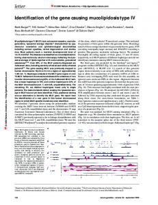
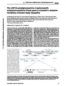
of the fear that this model is too restrictive (and consequently that distN Phardness is weak evidence for typical-case hardness), we seek a maximalistic model of distributions that may occur in practice. Such a model is provided by the notion of polynomial-time sampleable ensembles (underlying Definition 12). Our maximality thesis is based on the belief that the real world should be modeled as a feasible randomized process (rather than as an arbitrary process). This belief implies that all objects encountered in the world may be viewed as samples generated by a feasible randomized process. Definition 12 (sampleable ensembles and the class sampN P): We say that a probability ensemble X = {Xn }n∈N is (polynomial-time) sampleable if there exists a probabilistic polynomial-time algorithm A such that for every x ∈ {0, 1}∗ it holds that Pr[A(1|x| ) = x] = Pr[X|x| = x]. We denote by sampN P the class of distributional problems consisting of decision problems in N P coupled with sampleable probability ensembles. We first note that all simple probability ensembles are indeed sampleable, and thus distN P ⊆ sampN P. On the other hand, there exist sampleable probability ensembles that do not seem simple (and so it seems that distN P ⊂ sampN P). Extending the scope of distributional problems (from distN P to sampN P) facilitates the presentation of complete distributional problems. We first note that it is easy to prove that every natural NP-complete problem has a distributional version in sampN P that is distN P-hard. Furthermore, it is possible to prove that all natural NP-complete problem have distributional versions that are sampN P-complete. (In both cases, “natural” means that the corresponding Karp-reductions do not shrink the input, which is a weaker condition than the one in Proposition 6.) Theorem 13 (sampN P-completeness): Suppose that S ∈ N P and that every set in N P is reducible to S by a Karp-reduction that does not shrink the input. Then, there exists a polynomial-time sampleable ensemble X such that any problem in sampN P is reducible to (S, X) The proof of Theorem 13 is based on the observation that there exists a polynomialtime sampleable ensemble that dominates all polynomial-time sampleable ensembles. The existence of this ensemble is based on the notion of a universal (sampling) machine. Theorem 13 establishes a rich theory of sampN P-completeness, but does not relate this theory to the previously presented theory of distN P-completeness (see Figure 1). This is essentially done in the next theorem, which asserts that the existence of typically hard problems in sampN P implies their existence in distN P. Theorem 14 (sampN P-completeness versus distN P-completeness): If sampN P is not contained in tpcBPP then distN P is not contained in tpcBPP. Thus, the two “typical-case complexity” versions of the P-vs-NP Question are equivalent. That is, if some “sampleable distribution” versions of NP are not
123
tpcBPP sampNP
distNP sampNP-complete [Thm 13]
distNP-complete [Thms 5 and 7]
Fig. 1. Two types of average-case completeness
typically feasible then some “simple distribution” versions of NP are not typically feasible. In particular, if sampN P-complete problems are not in tpcBPP then distN P-complete problems are not in tpcBPP. The foregoing assertions would all follow if sampN P were (randomly) reducible to distN P (i.e., if every problem in sampN P were reducible (under a randomized version of Definition 3) to some problem in distN P); but, unfortunately, we do not know whether such reductions exist. Yet, underlying the proof of Theorem 14 is a more liberal notion of a reduction among distributional problems. Proof Sketch: We shall prove that if distN P is contained in tpcBPP then the same holds for sampN P (i.e., sampN P is contained in tpcBPP). Relying on Theorem 11 and an analogous result for the sampleable classes, it suffices to show that if distPC is contained in tpcBPPF, then the sampleable version of distPC, denoted sampPC, is contained in tpcBPPF. This will be shown by showing that, under a relaxed notion of a randomized reduction, every problem in sampPC is reduced to some problem in distPC. Loosely speaking, this relaxed notion (of a randomized reduction) only requires that the validity and domination conditions (of Definition 3 (when adapted to randomized reductions)) hold with respect to a noticeable fraction of the probability space of the reduction.23 We start by formulating this notion, when referring to distributional search problems. Definition: A relaxed reduction of the distributional problem (R, X) to the distributional problem (T, Y ) is a probabilistic polynomial-time oracle machine M that satisfies the following conditions with respect to a family of sets {Ωx ⊆ {0, 1}m(|x|) : x ∈ {0, 1}∗ }, where m(|x|) = poly(|x|) denotes an upper-bound on the number of the internal coin tosses of M on input x: 23
We warn that the existence of such a relaxed reduction between two specific distributional problems does not necessarily imply the existence of a corresponding (standard average-case) reduction. Specifically, although standard validity can be guaranteed (for problems in PC) by repeated invocations of the reduction, such a process will not redeem the violation of the standard domination condition.
124
Density (of Ωx ): There exists a noticeable function ρ : N → [0, 1] (i.e., ρ(n) > 1/poly(n)) such that, for every x ∈ {0, 1}∗, it holds that |Ωx | ≥ ρ(|x|)·2m(|x|) . Validity (with respect to Ωx ): For every r ∈ Ωx the reduction yields a correct answer; that is, M T (x, r) ∈ R(x) if R(x) 6= ∅ and M T (x, r) = ⊥ otherwise, where M T (x, r) denotes the execution of M on input x, internal coins r, and oracle access to T . Domination (with respect to Ωx ): There exists a positive polynomial p such that, for every y ∈ {0, 1}∗ and every n ∈ N, it holds that Pr[Q′ (Xn ) ∋ y] ≤ p(|y|) · Pr[Y|y| = y],
(5)
where Q′ (x) is a random variable, defined over the set Ωx , representing the set of queries made by M on input x, coins in Ωx , and oracle access to T . That is, Q′ (x) is defined by uniformly selecting r ∈ Ωx and considering the set of queries made by M on input x, internal coins r, and oracle access to T . (In addition, as in Definition 3, we also require that the reduction does not make too short queries.) The reader may verify that this relaxed notion of a reduction preserves typical feasibility; that is, for R ∈ PC, if there exists a relaxed reduction of (R, X) to (T, Y ) and (T, Y ) is in tpcBPPF then (R, X) is in tpcBPPF. The key observation is that the analysis may discard the case that, on input x, the reduction selects coins not in Ωx . Indeed, the queries made in that case may be untypical and the answers received may be wrong, but this is immaterial. What matter is that, on input x, with noticeable probability the reduction selects coins in Ωx , and produces “typical with respect to Y ” queries (by virtue of the relaxed domination condition). Such typical queries are answered correctly by the algorithm that typically solves (T, Y ), and if x has a solution then these answers yield a correct solution to x (by virtue of the relaxed validity condition). Thus, if x has a solution then with noticeable probability the reduction outputs a correct solution. On the other hand, the reduction never outputs a wrong solution (even when using coins not in Ωx ), because incorrect solutions are detected by relying on R ∈ PC. Our goal is presenting, for every (R, X) ∈ sampPC, a relaxed reduction of (R, X) to a related problem (R′ , X ′ ) ∈ distPC. (We use the standard notation X = {Xn }n∈N and X ′ = {Xn′ }n∈N .) An oversimplified case: For starters, suppose that Xn is uniformly distributed on some set Sn ⊆ {0, 1}n and that there is a polynomial-time computable and invertible mapping µ of Sn to {0, 1}ℓ(n), where ℓ(n) = log2 |Sn |. Then, mapping ′ x to 1|x|−ℓ(|x|)0µ(x), we obtain a reduction of (R, X) to (R′ , X ′ ), where Xn+1 n−ℓ(n) ℓ(n) ′ n−ℓ(n) −1 is uniform over {1 0v : v ∈ {0, 1} } and R (1 0v) = R(µ (v)) (or, equivalently, R(x) = R′ (1|x|−ℓ(|x|)0µ(x))). Note that X ′ is a simple ensemble and R′ ∈ PC; hence, (R′ , X ′ ) ∈ distPC. Also note that the foregoing mapping is indeed a valid reduction (i.e., it satisfies the efficiency, validity, and domination conditions). Thus, (R, X) is reduced to a problem in distPC (and indeed the relaxation was not used here).
125
A simple but more instructive case: Next, we drop the assumption that there is a polynomial-time computable and invertible mapping µ of Sn to {0, 1}ℓ(n), but maintain the assumption that Xn is uniform on some set Sn ⊆ {0, 1}n and assume that |Sn | = 2ℓ(n) is easily computable (from n). In this case, we may map x ∈ {0, 1}n to its image under a suitable randomly chosen hashing function h, which in particular maps n-bit strings to ℓ(n)-bit strings. That is, we randomly map x to (h, 1n−ℓ(n) 0h(x)), where h is uniformly selected in a set ℓ(n) Hn of suitable hash functions (i.e., pairwise independent ones). This calls for redefining R′ such that R′ (h, 1n−ℓ(n) 0v) corresponds to the preimages of v under h that are in Sn . Assuming that h is a 1-1 mapping of Sn to {0, 1}ℓ(n), we may define R′ (h, 1n−ℓ(n) 0v) = R(x) such that x is the unique string satisfying x ∈ Sn and h(x) = v, where the condition x ∈ Sn may be verified by providing the internal coins of the sampling procedure that generate x. Denoting the sampling procedure of X by S, and letting S(1n , r) denote the output of S on input 1n and internal coins r, we actually redefine R′ as R′ (h, 1n−ℓ(n) 0v) = {hr, yi : h(S(1n , r)) = v ∧ y ∈ R(S(1n , r))}.
(6)
We note that hr, yi ∈ R′ (h, 1|x|−ℓ(|x|)0h(x)) yields a desired solution y ∈ R(x) if S(1|x| , r) = x, but otherwise “all bets are off” (since y will be a solution for S(1|x| , r) 6= x). Now, although typically h will not be a 1-1 mapping of Sn to {0, 1}ℓ(n), it is the case that for each x ∈ Sn , with constant probability over the choice of h, it holds that h(x) has a unique preimage in Sn under h. In this case hr, yi ∈ R′ (h, 1|x|−ℓ(|x|)0h(x)) implies S(1|x| , r) = x (which, in turn, implies y ∈ R(x)). We claim that the randomized mapping of x to (h, 1n−ℓ(n) 0h(x)), ℓ(|x|) where h is uniformly selected in H|x| , yields a relaxed reduction of (R, X) ℓ(n)
to (R′ , X ′ ), where Xn′ ′ is uniform over Hn × {1n−ℓ(n) 0v : v ∈ {0, 1}ℓ(n)}. Needless to say, the claim refers to the reduction that (on input x, makes the query (h, 1n−ℓ(n) 0h(x)), and) returns y if the oracle answer equals hr, yi and y ∈ R(x). ℓ(|x|) The claim is proved by considering the set Ωx of choices of h ∈ H|x| for which x ∈ Sn is the only preimage of h(x) under h that resides in Sn (i.e., |{x′ ∈ Sn : h(x′ ) = h(x)}| = 1). In this case (i.e., h ∈ Ωx ) it holds that hr, yi ∈ R′ (h, 1|x|−ℓ(|x|)0h(x)) implies that S(1|x| , r) = x and y ∈ R(x), and the (relaxed) validity condition follows. The (relaxed) domination condition follows by noting that Pr[Xn = x] ≈ 2−ℓ(|x|), that x is mapped to (h, 1|x|−ℓ(|x|)0h(x)) with ℓ(|x|) probability 1/|H|x| |, and that x is the only preimage of (h, 1|x|−ℓ(|x|)0h(x)) under the mapping (among x′ ∈ Sn such that Ωx′ ∋ h). Before going any further, let us highlight the importance of hashing Xn to ℓ(n)-bit strings. On one hand, this mapping is “sufficiently” one-to-one, and thus (with constant probability) the solution provided for the hashed instance (i.e., h(x)) yield a solution for the original instance (i.e., x). This guarantees the validity of the reduction. On the other hand, for a typical h, the mapping of Xn to h(Xn ) covers the relevant range almost uniformly. This guarantees that the reduction satisfies the domination condition. Note that these two phenomena
126
impose conflicting requirements that are both met at the correct value of ℓ; that is, the one-to-one condition requires ℓ(n) ≥ log2 |Sn |, whereas an almost uniform cover requires ℓ(n) ≤ log2 |Sn |. Also note that ℓ(n) = log2 (1/Pr[Xn = x]) for every x in the support of Xn ; the latter quantity will be in our focus in the general case. The general case: Finally, we get rid of the assumption that Xn is uniformly distributed over some subset of {0, 1}n . All that we know is that there exists a probabilistic polynomial-time (“sampling”) algorithm S such that S(1n ) is distributed identically to Xn . In this (general) case, we map instances of (R, X) according to their probability mass such that x is mapped to an instance (of R′ ) that consists of (h, h(x)) and additional information, where h is a random hash function mapping n-bit long strings to ℓx -bit long strings such that def
ℓx = ⌈log2 (1/Pr[X|x| = x])⌉.
(7)
Since (in the general case) there may be more than 2ℓx strings in the support of Xn , we need to augment the reduced instance in order to ensure that it is uniquely associated with x. The basic idea is augmenting the mapping of x to (h, h(x)) with additional information that restricts Xn to strings that occur with probability at least 2−ℓx . Indeed, when Xn is restricted in this way, the value of h(Xn ) uniquely determines Xn . Let q(n) denote the randomness complexity of S and S(1n , r) denote the output of S on input 1n and internal coin tosses r ∈ {0, 1}q(n) . Then, we randomly map x to (h, h(x), h′ , v ′ ), where h : {0, 1}|x| → {0, 1}ℓx and h′ : {0, 1}q(|x|) → {0, 1}q(|x|)−ℓx are random hash functions and v ′ ∈ {0, 1}q(|x|)−ℓx is uniformly distributed. The instance (h, v, h′ , v ′ ) of the redefined search problem R′ has solutions that consists of pairs hr, yi such that h(S(1n , r)) = v ∧ h′ (r) = v ′ and y ∈ R(S(1n , r)). As we shall see, this augmentation guarantees that, with constant probability (over the choice of h, h′ , v ′ ), the solutions to the reduced instance (h, h(x), h′ , v ′ ) correspond to the solutions to the original instance x. The foregoing description assumes that, on input x, we can efficiently determine ℓx , which is an assumption that cannot be justified. Instead, we select ℓ uniformly in {0, 1, ..., q(|x|)}, and so with noticeable probability we do select the correct value (i.e., Pr[ℓ = ℓx ] = 1/(q(|x|)+1) = 1/poly(|x|)). For clarity, we make n and ℓ explicit in the reduced instance. Thus, we randomly map x ∈ {0, 1}n to ′ q(n)−ℓ (1n , 1ℓ , h, h(x), h′ , v ′ ) ∈ {0, 1}n , where ℓ ∈ {0, 1, ..., q(n)}, h ∈ Hnℓ , h′ ∈ Hq(n) , and v ′ ∈ {0, 1}q(n)−ℓ are uniformly distributed in the corresponding sets.24 This mapping will be used to reduce (R, X) to (R′ , X ′ ), where R′ and X ′ = {Xn′ ′ }n′ ∈N are redefined (yet again). Specifically, we let R′ (1n , 1ℓ , h, v, h′ , v ′ ) = {hr, yi : h(S(1n , r)) = v ∧ h′ (r) = v ′ ∧ y ∈ R(S(1n , r))} (8) 24
As in other places, a suitable encoding will be used such that the reduction maps strings of the same length to strings of the same length (i.e., n-bit string are mapped to n′ -bit strings, for n′ = poly(n)). For example, we may encode h1n , 1ℓ , h, h(x), h′ , v ′ i as 1n 01ℓ 01q(n)−ℓ 0hhihh(x)ihh′ ihv ′ i, where each hwi denotes an encoding of w by a string of length (n′ − (n + q(n) + 3))/4.
127
and Xn′ ′ assigns equal probability to each Xn′ ,ℓ (for ℓ ∈ {0, 1, ..., n}), where each q(n)−ℓ Xn′ ,ℓ is isomorphic to the uniform distribution over Hnℓ × {0, 1}ℓ × Hq(n) × {0, 1}q(n)−ℓ. Note that indeed (R′ , X ′ ) ∈ distPC. The foregoing randomized mapping is analyzed by considering the correct choice for ℓ; that is, on input x, we focus on the choice ℓ = ℓx . Under this conditioning (as we shall show), with constant probability over the choice of h, h′ and v ′ , the instance x is the only value in the support of Xn that is mapped to 6 ∅. It (1n , 1ℓx , h, h(x), h′ , v ′ ) and satisfies {r : h(S(1n , r)) = h(x) ∧ h′ (r) = v ′ } = follows that (for such h, h′ and v ′ ) any solution hr, yi ∈ R′ (1n , 1ℓx , h, h(x), h′ , v ′ ) satisfies S(1n , r) = x and thus y ∈ R(x), which means that the (relaxed) validity condition is satisfied. The (relaxed) domination condition is satisfied too, because (conditioned on ℓ = ℓx and for such h, h′ , v ′ ) the probability that Xn is mapped to (1n , 1ℓx , h, h(x), h′ , v ′ ) approximately equals Pr[Xn′ ′ ,ℓx = (1n , 1ℓx , h, h(x), h′ , v ′ )]. We now turn to analyze the probability, over the choice of h, h′ and v ′ , that the instance x is the only value in the support of Xn that is mapped to 6 ∅. (1n , 1ℓx , h, h(x), h′ , v ′ ) and satisfies {r : h(S(1n , r)) = h(x) ∧ h′ (r) = v ′ } = Firstly, we note that |{r : S(1n , r) = x}| ≥ 2q(n)−ℓx , and thus, with constant q(n)−ℓ probability over the choice of h′ ∈ Hq(n) x and v ′ ∈ {0, 1}q(n)−ℓx , there exists r that satisfies S(1n , r) = x and h′ (r) = v ′ . Furthermore, with constant probability q(n)−ℓ over the choice of h′ ∈ Hq(n) x and v ′ ∈ {0, 1}q(n)−ℓx , it also holds that there are at most O(2ℓx ) strings r such that h′ (r) = v ′ . Fixing such h′ and v ′ , we let Sh′ ,v′ = {S(1n , r) : h′ (r) = v ′ } and we note that, with constant probability over the choice of h ∈ Hnℓx , it holds that x is the only string in Sh′ ,v′ that is mapped to h(x) under h. Thus, with constant probability over the choice of h, h′ and v ′ , the instance x is the only value in the support of Xn that is mapped 6 ∅. to (1n , 1ℓx , h, h(x), h′ , v ′ ) and satisfies {r : h(S(1n , r)) = h(x) ∧ h′ (r) = v ′ } = The theorem follows.
Reflection: Theorem 14 implies that if sampN P is not contained in tpcBPP then every distN P-complete problem is not in tpcBPP. This means that the hardness of some distributional problems that refer to sampleable distributions implies the hardness of some distributional problems that refer to simple distributions. Furthermore, by Proposition 9, this implies the hardness of distributional problems that refer to the uniform distribution. Thus, hardness with respect to some distribution in an utmost wide class (which arguably captures all distributions that may occur in practice) implies hardness with respect to a single simple distribution (which arguably is the simplest one).
Relation to one-way functions. We note that the existence of one-way functions (see, e.g., [5, Chap. 2]) implies the existence of problems in sampPC that are not in tpcBPPF (which in turn implies the existence of such problems in distPC). Specifically, for a length-preserving one-way function f , consider the distribu-
128
tional search problem (Rf , {f (Un )}n∈N ), where Rf = {(f (r), r) : r ∈ {0, 1}∗}.25 On the other hand, it is not known whether the existence of a problem in sampPC\tpcBPPF implies the existence of one-way functions. In particular, the existence of a problem (R, X) in sampPC \ tpcBPPF represents the feasibility of generating hard instances for the search problem R, whereas the existence of one-way function represents the feasibility of generating instance-solution pairs such that the instances are hard to solve. Indeed, the gap refers to whether or not hard instances can be efficiently generated together with corresponding solutions. Our world view is thus depicted in Figure 2, where lower levels indicate seemingly weaker assumptions.
one-way functions exist
distNP is not in tpcBPP (equiv., sampNP is not in tpcBPP)
P is different than NP Fig. 2. Worst-case vs average-case assumptions
Bibliographic Notes The theory of average-case complexity was initiated by Levin [10], who in particular proved Theorem 5. In light of the laconic nature of the original text [10], we refer the interested reader to a survey [4], which provides a more detailed exposition of the definitions suggested by Levin as well as a discussion of the considerations underlying these suggestions. As noted in Section 2.1, the current text uses a variant of the original definitions. In particular, our definition of “typical-case feasibility” differs from the original definition of “average-case feasibility” in totally discarding exceptional instances and in even allowing the algorithm to fail on them (and not merely run for an excessive amount of time). The alternative definition was suggested by several researchers, and appears as a special case of the general treatment provided in [2]. Turning to Section 2.2, we note that while the existence of distN P-complete problems (cf. Theorem 5) was established in Levin’s original paper [10], the exis25
Note that the distribution f (Un ) is uniform in the special case that f is a permutation over {0, 1}n .
129
tence of distN P-complete versions of all natural NP-complete decision problems (cf. Theorem 7) was established more than two decades later in [11]. Section 3 is based on [1, 8]. Specifically, Theorem 11 (or rather the reduction of search to decision) is due to [1] and so is the introduction of the class sampN P. A version of Theorem 14 was proven in [8], and our proof follows their ideas, which in turn are closely related to the ideas underlying the construction of pseudorandom generators based on any one-way function [7]. Recall that we know of the existence of problems in distN P that are hard provided sampN P contains hard problems. However, these distributional problems do not seem very natural (i.e., they either refer to somewhat generic decision problems such as Su or to somewhat contrived probability ensembles (cf. Theorem 7)). The presentation of distN P-complete problems that combine a more natural decision problem (like SAT or Clique) with a more natural probability ensemble is an open problem. A natural question at this point is what have we gained by relaxing the requirements. In the context of average-case complexity, the negative side seems more prevailing (at least in the sense of being more systematic). In particular, assuming the existence of one-way functions, every natural NP-complete problem has a distributional version that is (typical-case) hard, where this version refers to a sampleable ensemble (and, in fact, even to a simple ensemble). Furthermore, in this case, some problems in NP have hard distributional versions that refer to the uniform distribution.
References 1. S. Ben-David, B. Chor, O. Goldreich, and M. Luby. On the Theory of Average Case Complexity. Journal of Computer and System Science, Vol. 44 (2), pages 193–219, 1992. 2. A. Bogdanov and L. Trevisan. Average-case complexity. Foundations and Trends in Theoretical Computer Science, Vol. 2 (1), 2006. 3. S.A. Cook. The Complexity of Theorem Proving Procedures. In 3rd ACM Symposium on the Theory of Computing, pages 151–158, 1971. 4. O. Goldreich. Notes on Levin’s Theory of Average-Case Complexity. This volume. See also ECCC, TR97-058, Dec. 1997. 5. O. Goldreich. Foundation of Cryptography: Basic Tools. Cambridge University Press, 2001. 6. O. Goldreich. Computational Complexity: A Conceptual Perspective. Cambridge University Press, 2008. 7. J. H˚ astad, R. Impagliazzo, L.A. Levin and M. Luby. A Pseudorandom Generator from any One-way Function. SICOMP, Volume 28, Number 4, pages 1364–1396, 1999. Combines papers of Impagliazzo et al. (21st STOC, 1989) and H˚ astad (22nd STOC, 1990). 8. R. Impagliazzo and L.A. Levin. No Better Ways to Generate Hard NP Instances than Picking Uniformly at Random. In 31st IEEE Symposium on Foundations of Computer Science, pages 812–821, 1990. 9. R.M. Karp. Reducibility among Combinatorial Problems. In Complexity of Computer Computations, R.E. Miller and J.W. Thatcher (eds.), Plenum Press, pages 85–103, 1972.
130 10. L.A. Levin. Average Case Complete Problems. SIAM Journal on Computing, Vol. 15, pages 285–286, 1986. 11. N. Livne. All Natural NPC Problems Have Average-Case Complete Versions. ECCC, TR06-122, 2006.