Average-Optimal Single and Multiple Approximate String Matching

Average-Optimal Single and Multiple Approximate String Matching KIMMO FREDRIKSSON University of Joensuu and GONZALO NAVARRO University of Chile We present a new algorithm for multiple approximate string matching. It is based on reading backwards enough `-grams from text windows so as to prove that no occurrence can contain the part of the window read, and then shifting the window. We show analytically that our algorithm is optimal on average. Hence our first contribution is to fill an important gap in the area, since no average-optimal algorithm existed for multiple approximate string matching. We consider several variants and practical improvements to our algorithm, and show experimentally that they are resistant to the number of patterns and the fastest for low difference ratios, displacing the long-standing best algorithms. Hence our second contribution is to give a practical algorithm for this problem, by far better than any existing alternative in many cases of interest. On real life texts, our algorithm is especially interesting for computational biology applications. In particular, we show that our algorithm can be successfully used to search for one pattern, where many more competing algorithms exist. Our algorithm is also average-optimal in this case, being the second after that of Chang and Marr. However, our algorithm permits higher difference ratios than Chang and Marr, and this is our third contribution. In practice, our algorithm is competitive in this scenario too, being the fastest for low difference ratios and moderate alphabet sizes. This is our fourth contribution, which also answers affirmatively the question of whether a practical average-optimal approximate string matching algorithm existed. Categories and Subject Descriptors: F.2.2 [Analysis of algorithms and problem complexity]: Nonnumerical Algorithms and Problems—Pattern matching, Computations on discrete structures; H.3.3 [Information storage and retrieval]: Information Search and Retrieval—Search process General Terms: Algorithms, Theory Additional Key Words and Phrases: Algorithms, approximate string matching, optimality

Supported by the Academy of Finland, grant 202281 (first author), partially supported by Fondecyt grant 1-020831 (second author). Authors’ address: Kimmo Fredriksson, Department of Computer Science, P.O. Box 111, FI80101 Joensuu, Finland. Email: [email protected]. Gonzalo Navarro, Department of Computer Science, University of Chile, Blanco Encalada 2120, Santiago, Chile. Email: [email protected]. Permission to make digital/hard copy of all or part of this material without fee for personal or classroom use provided that the copies are not made or distributed for profit or commercial advantage, the ACM copyright/server notice, the title of the publication, and its date appear, and notice is given that copying is by permission of the ACM, Inc. To copy otherwise, to republish, to post on servers, or to redistribute to lists requires prior specific permission and/or a fee. c 20YY ACM 0000-0000/20YY/0000-0001 $5.00 ° ACM Journal Name, Vol. V, No. N, Month 20YY, Pages 1–45.

2

·

K. Fredriksson and G. Navarro

1. INTRODUCTION Approximate string matching is one of the main problems in classical string algorithms, with applications to text searching, computational biology, pattern recognition, etc. Given a text T1...n , a pattern P1...m , and a maximal number of differences permitted, k, we want to find all the text positions where the pattern matches the text up to k differences. The differences can be substituting, deleting or inserting a character. We call α = k/m the difference ratio, and σ the size of the alphabet Σ. A natural extension to the basic problem consists of multipattern searching, that is, searching for r patterns P 1 . . . P r simultaneously in order to report all their occurrences with at most k differences. This has also several applications such as virus and intrusion detection [Kumar and Spafford 1994], spelling [Kukich 1992], speech recognition [Dixon and Martin 1979], optical character recognition [Elliman and Lancaster 1990], handwriting recognition [Lopresti and Tomkins 1994], text retrieval under synonym or thesaurus expansion [Baeza-Yates and Ribeiro-Neto 1999], computational biology [Sankoff and Kruskal 1983; Waterman 1995], multidimensional approximate matching [Baeza-Yates and Navarro 2000], batch processing of single-pattern approximate searching, etc. Moreover, some single-pattern approximate search algorithms resort to multipattern searching of pattern pieces [Navarro and Baeza-Yates 2001]. Depending on the application, r may vary from a few to thousands of patterns. The naive approach is to perform r separate searches, so the goal is to do better. In this paper we use the terms “approximate matching” and “approximate searching” indistinctly, meaning the search for approximate occurrences of short strings (the patterns) inside a longer string (the text). This is one particular case of the wider concept of sequence alignment, pervasive in computational biology. Actually, the area of sequence alignment is divided into global alignment (where two strings are wholly compared), semi-global alignment (where one string is compared against any substring of the other, our focus in this paper), and local alignment (where all substrings of both strings are compared). Multiple alignment refers to comparing a set of strings so as to find common parts to all of them. Note that this is quite different from multiple string matching, where many (pattern) strings are compared against one (the text). For average case analyses of text search algorithms it is customary to assume random text and patterns drawn over a uniformly distributed alphabet. Averagecase complexity thus refers to averaging the cost of an algorithm over all possible texts of length n and patterns of length m, giving equal weight to each combination. The average complexity of a problem refers to the best possible average case of an algorithm solving the problem, and an average-optimal algorithm is one whose average-case complexity matches the average complexity of the problem. The single-pattern problem has received a lot of attention since the sixties [Navarro 2001]. After the first dynamic-programming-based O(mn) time solution to the problem [Sellers 1980], many faster techniques have been proposed, both for the worst and the average case. For low difference ratios (the most interesting case) the so-called filtration algorithms are the most efficient ones. These algorithms discard most of the text by checking for a necessary condition, and use another algorithm to verify the text areas that cannot be discarded. For filtration algoACM Journal Name, Vol. V, No. N, Month 20YY.

Average-Optimal Single and Multiple Approximate String Matching

·

3

rithms, the two important parameters are the filtration speed and the maximum difference ratio α up to which they work. Note that, in any case, one needs a good non-filtration algorithm to verify the text that the filter cannot discard. The best non-filtration algorithms are in practice by Baeza-Yates & Navarro [Baeza-Yates and Navarro 1999; Navarro and Baeza-Yates 2001], and by Myers [Myers 1999], with average complexities of O(kmn/w) and O(kn/w), respectively, where w is the length in bits of the computer word. In 1994, Chang & Marr [Chang and Marr 1994] showed that the average complexity of the problem is O((k + logσ m)n/m), and gave the first (filtration) algorithm that achieved that average√ optimal cost for α < 1/3 − O(1/ σ). In practice, the fastest algorithms, based on filtration, have a complexity of O(k logσ (m)n/m) and work for α < 1/ logσ m [Navarro and Baeza-Yates 1999]. Hence the quest for an average-optimal algorithm whose optimality shows up in practice has been advocated [Navarro and Raffinot 2002]. The multipattern problem has received much less attention, not because of lack of interest but because of its difficulty. There exist algorithms that search permitting only k = 1 difference [Muth and Manber 1996], that handle too few patterns [BaezaYates and Navarro 2002], that handle only low difference ratios [Baeza-Yates and Navarro 2002], and that handle only very short patterns [Hyyrö et al. 2004]. No effective algorithm exists to search for many patterns with intermediate difference ratio. Moreover, as the number of patterns grows, the difference ratios that can be handled get reduced, as the most effective algorithm [Baeza-Yates and Navarro 2002] works for α < 1/ logσ (rm). No optimal algorithms have been devised, and the existing algorithms are not that fast. Hence multiple approximate string matching is a rather undeveloped area. In this paper we present several contributions to the approximate search problem, for a single pattern and for multiple patterns: —We present a new algorithm for multiple approximate string matching. It is based on sliding a window over the text. At each window, we read backwards successive `-grams until we can prove that no pattern occurrence can contain those `-grams read. This is done by a preprocessing that counts the minimum number of differences needed to match each `-gram inside any pattern. Then the window is displaced far enough to avoid containing the scanned `-grams. —We show analytically that the average √ complexity of our algorithm is O((k + logσ (rm))n/m) for α < 1/2 − O(1/ σ). We show that this is average-optimal, which makes our algorithm the first average-optimal multiple approximate string matching algorithm. If applied to a single pattern, the algorithm is also optimal, like that of Chang & Marr. However, our algorithm works√for higher difference ratios, since Chang & Marr works only for α < 1/3 − O(1/ σ). —We consider several practical improvements to our algorithm, such as optimal choice of the window `-grams, reduction of the cost to check windows that cannot be discarded, reduction of preprocessing costs for many patterns, and so on. As a result, our algorithm turns out to be very competitive in practice, apart from theoretically optimal. —We perform exhaustive experiments to evaluate the different aspects of our algorithm and to compare it against others. We show that our algorithm is resistant ACM Journal Name, Vol. V, No. N, Month 20YY.

4

·


to the number of patterns and that it works well for low difference ratios. In these cases, our algorithm displaces the long-standing best algorithms [Muth and Manber 1996; Baeza-Yates and Navarro 2002] (since 1996) in most cases, largely improving their search times. Our algorithm is competitive even to search for one single pattern, where many more competing alternatives exist. In this case our algorithm becomes the fastest choice for low difference ratios and not very large alphabets. On real life texts, we show that our algorithm is especially interesting for computational biology applications (searching dna and proteins). —As a side contribution, we explore several variants of our algorithm, which turn out to be more or less direct extensions to multipattern searching of Chang & Marr [Chang and Marr 1994], let by Chang & Lawler [Chang and Lawler 1994], laq by Sutinen & Tarhio [Sutinen and Tarhio 1996]. We also consider combining the basic idea of laq with our main algorithm. In most cases our new algorithm is superior, although these variants are of interest in some particular situations. Hence we have positively settled the question of the existence of a practical average-optimal approximate string matching algorithm [Navarro and Raffinot 2002]. It is interesting that our algorithm is theoretically optimal for low and intermediate difference ratios, but good in practice only for low difference ratios. The reason has to do with the space requirement of our algorithm, that is polynomial but high, and that forces us in practice to use suboptimal parameter settings. Preliminary partial versions of this paper appeared in [Fredriksson and Navarro 2003; 2004]. 2. RELATED WORK In this section we cover the existing algorithms for multiple approximate string matching, as well as the techniques for simple approximate string matching that are relevant to our work. We explain them up to the level necessary to understand their relevance for us. 2.1 Multiple Approximate String Matching The naive approach to multipattern approximate searching is to perform r separate searches, one per pattern. If we use the optimal single-pattern algorithm [Chang and Marr 1994], the average search time becomes O((k+logσ m)rn/m) for the naive approach. On the other hand, if we use the classical O(mn) algorithm [Sellers 1980] the time is O(rmn). Few algorithms exist for multipattern approximate searching under the k differences model. The first one was presented by Muth and Manber [Muth and Manber 1996]. It permits searching with k = 1 differences only, but it is rather tolerant to the number of patterns r, which can reach the hundreds without affecting much the cost of the search. They show that, if an approximate occurrence of P in T ends at position j and we take P 0 = Tj−m+1...j , then there are character positions s and s0 such that P and P 0 become equal if we remove their s-th and s0 -th character, respectively. Therefore they take all the m choices of removing a single character of every pattern P i and store the rm strings in a hash table. Later, they consider every text window of the form Tj−m+1...j , and for each of the m choices of removing a single window character, they search for the resulting substring in ACM Journal Name, Vol. V, No. N, Month 20YY.


·

5

the hash table. If the substring is found in the table, they check the appropriate pattern in the text window. The preprocessing time is O(rm) and the average search time is O(mn(1 + rm2 /M )), where M is the size of the hash table. This adds up O(rm + nm(1 + rm2 /M )), which is O(m(r + n)) if M = Ω(m2 r). The time is basically independent of r if n is large enough. However, in order to permit a general number k of differences, they should consider every way of removing k characters from the windows, resulting in an O(mk (r + n)) time algorithm, which is clearly impractical for all but very small k values. Baeza-Yates and Navarro [Baeza-Yates and Navarro 2002] have presented several algorithms for this problem. One of them, partitioning into exact search, uses the fact that, if P is cut into k + 1 pieces, then at least one of the pieces appears inside every occurrence with no differences. Hence the algorithm splits every pattern into k + 1 pieces and searches for the r(k + 1) pieces with an exact multipattern search algorithm. The preprocessing takes O(rm) time. If they used an optimal multipattern exact search algorithm like MultiBDM [Crochemore and Rytter 1994], the search time would have been O(k logσ (rm)n/m) on average. For practical reasons they used another algorithm, more suitable to searching for short pieces (of length bm/(k + 1)c), albeit with worse theoretical complexity. This technique can be applied for α < 1/ logσ (rm), a limit that gets stricter as m or r increase. They also presented other algorithms that, although can handle higher difference ratios, are linear on r, which means that they give a speedup only up to a constant number c of patterns and then just divide the search into r/c groups that are searched for separately. Superimposition uses a standard search technique on a set of “superimposed” patterns, which means that the i-th character of the superimposition matches the i-th character of any of the superimposed patterns. Implemented over a newer bit-parallel algorithm [Myers p 1999], superimposition would yield average time O(rn/(σ(1−α)2 )) for α < 1−e r/σ on patterns shorter than the number of bits in the computer word, w (typically w = 32 or 64). Different techniques are used to cope with longer patterns, but the times are worse. Counting extends a single-pattern algorithm that slides a window of length m over the text checking in linear time whether it shares at least m − k characters with the pattern (regardless of the order). The multipattern version keeps several counters in a single computer word, achieving an average search time of O(rn log(m)/w) for α < e−m/σ . Hyyrö et al. [Hyyrö et al. 2004] have recently presented another bit-parallel technique to simultaneously search for a few short patterns. When m ≤ w, they need O(dr/bw/mcen) worst-case time instead of O(rn). On average this improves to O(dr/bw/ max(k, log m)cen). 2.2 Dynamic Programming and Myers’ Bit-parallel Algorithm The classical algorithm to find the approximate occurrences of pattern P inside text T [Sellers 1980] is to compute a matrix Ci,j for 0 ≤ i ≤ m and 0 ≤ j ≤ n, using dynamic programming as follows: Ci,0 = i ,

C0,j

=

0

Ci+1,j+1 = if Pi+1 = Tj+1 then Ci,j else 1 + min(Ci,j , Ci,j+1 , Ci+1,j ) ACM Journal Name, Vol. V, No. N, Month 20YY.

6

·


which can be computed, for example, column-wise. We need only the previous column in order to compute the current one. Every time the current column value Cm,j ≤ k we report text position j as the endpoint of an occurrence. The algorithm needs O(mn) time and O(m) space. The same matrix can be used to compute the edit distance (number of differences necessary to convert one string into the other) just by changing C0,j = j in the initial conditions. The distance is then Cm,n . One of the most successful non-filtration approximate string matching algorithms consists of a bit-parallel version of the dynamic programming matrix [Myers 1999]. On a computer word of w bits, the algorithm obtains O(mn/w) search time. The central idea is to represent the current column C∗,j using two streams of m bits, one indicating positive and the other negative differences of the form Ci,j − Ci−1,j . Since consecutive cells in C differ at most by ±1, this representation is sufficient. Myers manages to update those vectors in constant time per column. 2.3 The Algorithm of Tarhio and Ukkonen Tarhio and Ukkonen [Tarhio and Ukkonen 1993; Jokinen et al. 1996] presented the first filtration algorithm (1991), using a Boyer-Moore-like technique to filter the text. The idea is to align the pattern with a text window and scan the text backwards. The scanning ends where more than k “bad” text characters are found. A “bad” character is one that not only does not match the pattern position it is aligned with, but it also does not match any pattern character at a distance of k characters or less. More formally, assume that the window starts at text position j + 1, and therefore Tj+i is aligned with Pi . Then Tj+i is bad when Bad(i, Tj+i ), where Bad(i, c) has been precomputed as c 6∈ {Pi−k , Pi−k+1 , ..., Pi , ...Pi+k }. The idea of the bad characters is that we know for sure that we have to pay a difference to match them, that is, they will not match as a byproduct of inserting or deleting other characters. When more than k characters that are differences for sure are found, the current text window can be abandoned and shifted forward. If, on the other hand, the beginning of the window is reached, the area Tj+1−k..j+m must be checked with a classical algorithm. To know how much can we shift the window, the authors show that there is no point in shifting P to a new position j 0 where none of the k + 1 text characters that are at the end of the current window (Tj+m−k , ...Tj+m ) match the corresponding character of P , that is, where Tj+m−s 6= Pm−s−(j 0 −j) . If those differences are fixed with substitutions we make k + 1 differences, and if they can be fixed with less than k + 1 operations, then it is because we aligned some of the involved pattern and text characters using insertions and deletions. In this case, we would have obtained the same effect aligning the matching characters from start. So for each pattern position i ∈ {m − k..m} and each text character a that could be aligned to position i (that is, for all a ∈ Σ) the shift to align a in the pattern is precomputed, that is, Shif t(i, a) = mins>0 {Pi−s = a} (or m if no such s exists). Later, the shift for the window is computed as mini∈m−k..m Shif t(i, Tj+i ). This last minimum is computed together with the backward window traversal. The (simplified) analysis [Tarhio and Ukkonen 1993; Navarro 2001] shows that the search time is O(k 2 n/σ), for α < e−(2k+1)/σ . The analysis is valid for m À σ > k. The algorithm is competitive in practice for low difference ratios. Interestingly, the ACM Journal Name, Vol. V, No. N, Month 20YY.


·

7

version k = 0 corresponds exactly to Horspool algorithm [Horspool 1980]. Like Horspool, it does not take proper advantage of very long patterns. 2.4 The Algorithm of Chang and Marr Chang and Marr [Chang and Marr 1994] show that no approximate search algorithm for a single pattern can be faster than O((k + logσ m)n/m) on the average. This is not hard to prove, and we give more details in Section 4. In the same paper [Chang and Marr 1994], Chang and Marr presented an algorithm achieving that optimal average time complexity. In the preprocessing phase they build a table D as follows. They choose a number ` in the range 1 ≤ ` ≤ d(m − k)/2e, whose exact value we will consider shortly. For every string S of length ` (`-gram), they search for S in P and store in D[S] the smallest number of differences needed to match S inside P (this is a number between 0 and `). Hence D requires space for σ ` entries and is computed in σ ` `m time. A numerical representation of Σ` permits constant time access to D. The text scanning phase consists of logically dividing the text into blocks of length b = d(m − k)/2e, which ensures that any approximate occurrence of P (which must be of length at least m−k) contains at least one whole block. Each block Tib+1...ib+b is processed as follows. They take the first `-gram of the block, S 1 = Tib+1...ib+` , and obtain D[S 1 ]. Then they take the next `-gram, S 2 = Tib+`+1...ib+2` , and obtain D[S 2 ], and so on. If, before reaching the end of the block, they have obtained P t 1≤t≤u D[S ] > k, then they can safely skip the block because no occurrence of P can contain the block, as merely matching those t `-grams anywhere inside P requires more than k differences. If, on the other hand, they reach the end of the block without surpassing k total differences, the block must be checked. In order to check for Tib+1...ib+b they run the classical dynamic programming algorithm over Tib+b+1−m−k...ib+m+k . In order to keep the space requirement polynomial in m, it is required that ` = O(logσ m). On the other hand, in order to achieve the claimed complexity, it is necessary that ` ≥ x logσ m for some constant x > √ 3, so the space is O(mx ). The optimal complexity holds as long as α < 1/3 − O(1/ σ). A somewhat related algorithm is let, by Chang & Lawler [Chang and Lawler 1994]. In this case the window is not fixed but slides over the text and they keep count of the minimum number of differences necessary to match the current window. To slide the window they include text at its right and discard from its left. let, however, does not permit approximate but just exact matching of the window substrings inside P , and therefore its tolerance to differences is lower. 2.5 The Approximate BNDM Algorithm Navarro and Raffinot [Navarro and Raffinot 2000] presented a novel approach based on suffix automata. A suffix automaton built over a string recognizes all the suffixes of the string. In [Navarro and Raffinot 2000], they adapted an exact string matching algorithm, BDM, to allow differences. The idea of the original BDM algorithm is as follows [Crochemore and Rytter 1994]. The deterministic suffix automaton of the reverse pattern is built, so it recognizes the reverse prefixes of the pattern. Then the pattern is aligned with a text window, and the window is scanned backwards with the automaton (this is ACM Journal Name, Vol. V, No. N, Month 20YY.

8

·


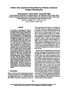
why the pattern is reversed). The automaton is active as long as what it has read is a substring of the pattern. Each time the automaton reaches a final state, it has seen a pattern prefix, so we remember the last time it happened. If the automaton arrives with active states to the beginning of the window then the pattern has been found, otherwise what is there is not a substring of the pattern and hence the pattern cannot be in the window. In any case the last window position that matched a pattern prefix gives the next initial window position. The algorithm BNDM [Navarro and Raffinot 2000] is a bit-parallel implementation of the nondeterministic suffix automaton, which is much faster in practice and allows searching for extended patterns. This nondeterministic automaton is then modified to match any suffix of the pattern with up to k differences, and then essentially the same BDM algorithm is applied. The window will be abandoned when no pattern substring matches with k differences what was read. The window is shifted to the next pattern prefix found with k differences. The matches must start exactly at the initial window position. The window length is m − k, not m, to ensure that if there is an occurrence starting at the window position then a substring of the pattern occurs in any suffix of the window (so we do not abandon the window before reaching the occurrence). Reaching the beginning of the window does not guarantee a match, however, so we have to check the area by computing edit distance from the beginning of the window (at most m + k text characters). In [Navarro 2001] it is shown that the algorithm inspects on average √ O(n(k + logσ (m)/m)) characters, and the filter works well for α < 1/2 − O(1/ σ). This looks optimal and works for higher difference ratios than Chang & Marr. However, characters cannot be inspected in constant time. In the original algorithm [Navarro and Raffinot 2000], the nondeterministic automaton is simulated in O(km/w) operations per character. Later [Hyyrö and Navarro 2002] this was improved to O(m/w) by adapting Myers’ bit-parallel simulation. However, optimality is attained only for m = O(w). In practice, the result is competitive for low difference ratios and for pattern lengths close to w. 3. OUR ALGORITHM We explain now the basic idea of our algorithm, and later consider different practical improvements. Given r search patterns P 1 . . . P r , the preprocessing fixes value ` (to be discussed later) and builds a table D : Σ` → N telling, for each possible `-gram, the minimum number of differences necessary to match the `-gram inside any of the patterns. Figure 1 illustrates. The scanning phase proceeds by sliding a window of length m − k over the text. The invariant is that any occurrence starting before the window has already been reported. For each window position i + 1 . . . i + m − k, we read successive `grams backwards, that is, S 1 = Ti+m−k−`+1...i+m−k , S 2 = Ti+m−k−2`+1...i+m−k−` , . . ., S t = Ti+m−k−t`+1...i+m−k−(t−1)` , and so on. Any occurrence starting at the beginning of the window must fully contain those P `-grams. We accumulate the D values for the successive `-grams read, Mu = 1≤t≤u D[S t ]. If, at some point, the ACM Journal Name, Vol. V, No. N, Month 20YY.

·


P 1 = aacaccgaaa

P 2 = gaacgaacac

9

P 3 = ttcggcccgg

aa

ac

ag

at

ca

cc

cg

ct

ga

gc

gg

gt

ta

tc

tg

tt

DP 1 DP 2 DP 3

0 0 2 ↓

0 0 1 ↓

1 1 1 ↓

1 1 1 ↓

0 0 1 ↓

0 1 0 ↓

0 0 0 ↓

1 1 1 ↓

0 0 1 ↓

1 1 0 ↓

1 1 0 ↓

1 1 1 ↓

1 1 1 ↓

1 1 0 ↓

1 1 1 ↓

2 2 0 ↓

D

0

0

1

1

0

0

0

1

0

0

0

1

1

0

1

0

Fig. 1. An example of the table D, computed for the set of three dna patterns and for ` = 2. For example, the 2-gram ga occurs in P 1 and P 2 with 0 errors and in P 3 with 1 error. The table D is obtained by taking the minimum of the table entries for each of the patterns.

Current window position is T25..33 : i T

...

24 c

25 c

26 t

27 a

28 g

29 g

30 t

31 a

32 a

33 t

34 t

35 t

36 a

37 c

...

42 a

43 g

...

M = D[T32...33 ] + D[T30..31 ] = D[at] + D[ta] = 2 > k ⇒ The window can be shifted past T [30]: i T

...

30 t

31 a

32 a

33 t

34 t

35 t

36 a

37 c

38 a

39 a

40 t

41 t

M = D[T38...39 ] + D[T36..37 ] + D[T34..35 ] + D[T32..33 ] = D[aa] + D[ac] + D[tt] + D[at] = 1 ≤ k ⇒ Must verify the area T31..41 . The next window position is T32..40 .

Fig. 2. An example of CanShift(24, D) using the D table of Figure 1. The parameters are m = 10, k = 1, and ` = 2.

sum Mu exceeds k, it is not possible to have an occurrence containing the sequence of `-grams read S u . . . S 1 , as merely matching those `-grams inside any pattern in any order needs more than k differences. Therefore, if at some point we obtain Mu > k, then we can safely shift the window to start at position i + m − k − t` + 2, which is the first position not containing the `-grams read. On the other hand, it might be that we read all the `-grams fully contained in the window and do not surpass threshold k. In this case we must check the text area of the window with a non-filtration algorithm, as it might contain an occurrence. We scan the text area Ti+1...i+m+k for each of the r patterns, so as to cover any possible occurrence starting at the beginning of the window and report any match found. Then, we shift the window by one position and resume the scanning. Figure 2 illustrates. The above scheme may report the same ending position of occurrence several ACM Journal Name, Vol. V, No. N, Month 20YY.

10

·


times, if there are several starting positions for it. A way to avoid this is to remember the last position scanned when verifying the text, c, so as to prevent retraversing the same text areas but just restarting from the point we left the last verification. We use Myers’ algorithm [Myers 1999] for the verification of single patterns, which makes the cost O(m2 /w) per pattern, being w the number of bits in the computer word. Figure 3 gives the code in its simplest form. We present next several improvements over the basic idea and change accordingly some modules of this code. Search is the main module, using variables i and c denoting the position preceding the first character of the window and the first position not yet verified, respectively. The verification algorithm must be reinitialized when verification must restart ahead of the last verified position, otherwise the last verification is resumed from position c. CanShift(i, D) considers window i + 1 . . . i + m − k and scans `-grams backwards from it until determining that it can be shifted or not. It returns a position pos such that the new window can start at position pos + 1. If pos = i it means that the window must be verified. Preprocess computes ` and D. The computation of ` takes the largest value such that it will not exceed the window length, the D table will fit in memory, and the preprocessing cost will not exceed the average search cost. Finally, MinDist(S, P ) computes the minimum edit distance of S inside P , using the formula of Section 2.2 to find the “pattern” S inside the “text” P . In this case 0 ≤ i ≤ ` and 0 ≤ j ≤ m, and it turns out to be more convenient for presenting our later developments to compute the matrix row-wise rather than column-wise. 3.1 Optimal Choice of `-grams The basic algorithm uses the last consecutive `-grams of the block in order to find more than k differences. This is simple, but not necessarily the best choice. Note that any set of non-overlapping `-grams found inside the window whose total number of differences inside P exceeds k permits us discarding the window. Hence the question of using the best possible set is raised. The optimization problem is as follows. Given the text window Ti+1...i+m−k we have m − k − ` + 1 possible `-grams, namely Ti+1...i+` , Ti+2...i+`+1 , . . ., Ti+m−k−`+1...i+m−kP . From this set we want a subset of non-overlapping `-grams S 1 . . . S u such that 1≤t≤u D[S t ] > k. Moreover, we want to process the set right to left and detect a good enough subset as soon as possible. This is solved by redefining Mu as the maximum sum that can be obtained using disjoint `-grams that start at positions i + u . . . i + m − k. Initially we start with Mu = 0 for m − k − ` + 2 < u ≤ m − k + 1. Then we traverse the block computing, for decreasing u values, Mu ←

max(D[Ti+u...i+u+`−1 ] + Mu+` , Mu+1 ),

(1)

where the first term accounts for the fact that we choose to use the `-gram that starts at u and add to it the best solution to the right that does not overlap this `-gram; and the second term accounts for the fact that we do not use the `-gram that starts at u. We compute Mu for decreasing u until either (i) Mu > k, in which case we shift the window, or (ii) u = 0, in which case we have to verify the window. Figure 4 ACM Journal Name, Vol. V, No. N, Month 20YY.


·

11

1 r Search (T1...n , P1...m . . . P1...m , k) 1. Preprocess ( ) 2. i ← 0, c ← 0 3. While i ≤ n − (m − k) Do 4. pos ← CanShift (i, D) 5. If pos = i Then 6. If i + 1 > c Then 7. Initialize verification algorithm 8. c←i+1 9. Run verification in text area Tc...i+m+k 10. c←i+m+k+1 11. pos ← pos + 1 12. i ← pos

CanShift (i, D) 1. M ←0 2. p←m−k 3. While p ≥ ` Do 4. p←p−` 5. M ← M + D[Ti+p+1...i+p+` ] 6. If M > k Then Return i + p + 1 7. Return i Preprocess ( ) 1. ` ← according to Eq. (4) 2. For S ∈ Σ` Do 3. D[S] ← ` 4. For i ∈ 1 . . . r Do 5. D[S] ← min(D[S], MinDist(S, P i )) MinDist (S1...` , P1...m ) 1. For j ∈ 0 . . . m Do Cj ← 0 2. For i ∈ 1 . . . ` Do 3. Cold ← C0 , C0 ← i 4. For j ∈ 1 . . . m Do 5. If Si = Pj Then Cnew ← Cold 6. Else Cnew ← 1 + min(Cold, Cj , Cj−1 ) 7. Cold ← Cj , Cj ← Cnew 8. Return min0≤j≤m Cj

Fig. 3. Simple description of the algorithm. The main variables are global in the rest of the paper, to simplify the presentation.

gives the code. Note that the cost of choosing the best set of `-grams is that, if we abandon the block after considering position x, then we work O(x/`) with the simple method and O(x) with the current one. (This assumes we can read an `-gram in constant time.) However, x itself may be smaller with the optimization method. ACM Journal Name, Vol. V, No. N, Month 20YY.

12

·


CanShift (i, D) 1. For u ∈ m − k − ` + 2 . . . m − k + 1 Do Mu ← 0 2. u←m−k−`+1 3. While u ≥ 0 Do 4. Mu ← max(D[Ti+u...i+u+`−1 ] + Mu+` , Mu+1 ) 5. If M > k Then Return i + u + 1 6. u←u−1 7. Return i

Fig. 4. Optimization technique to choose the set of overlapping `-grams that maximize the sum of differences. P1 P3

P2 P4

P1 P2

P3 P4

P1

Fig. 5.

P2

P3

P4

Pattern hierarchy for 4 patterns.

3.2 Hierarchical Verification On the windows that have to be verified, we could simply run the verification for every pattern, one by one. A more sophisticated choice is hierarchical verification (already presented in previous work [Baeza-Yates and Navarro 2002]). We form a tree whose nodes have the form [i, j] and represent the group of patterns P i . . . P j . The root is [1, r]. The leaves have the form [i, i]. Every internal node [i, j] has two children [i, b(i + j)/2c] and [b(i + j)/2c + 1, j]. The hierarchy is used as follows. For every internal node [i, j] we have a table D computed using the minimum distances between each `-gram and patterns P i . . . P j . This is done by computing first the leaves (that is, each pattern separately) and then computing every cell of D in the internal node as the minimum over the corresponding cell in its two children. In order to scan the text, we use the D table of the root node, which corresponds to the full set of patterns. Every time a window has to be verified with respect to a node in the hierarchy (at first, the root node), we rescan the window considering the two children of the current node. It is possible that the window can be discarded for both children, for one, or for none. We recursively repeat the process for every child that does not permit discarding the window, see Figure 5. If we process a leaf node and still have to verify the window, then we run the verification algorithm for the corresponding single pattern. The idea of using the hierarchy instead of plainly checking the r patterns one by one is that it is possible that the grouping of the patterns matches a block, but ACM Journal Name, Vol. V, No. N, Month 20YY.


·

13

PreprocessD (i) 1. For S ∈ Σ` Do 2. Di,i [S] ← MinDist(S, P i ) HierarchyPreprocess (i, j) 1. If i = j Then PreprocessD(i) 2. Else 3. p ← b(i + j)/2c 4. HierarchyPreprocess (i, p, S) 5. HierarchyPreprocess (p + 1, j, S) 6. For S ∈ Σ` Do 7. Di,j [S] ← min(Di,p [S], Dp+1,j [S]) Preprocess ( ) 1. ` ← according to Eq. (6) 2. HierarchyPreprocess(1, r)

Fig. 6. Preprocessing to build the hierarchy. It produces global tables Di,j to be used by HierarchyVerify. Table D is D1,r .

that none of its halves match. In this case we save verification time. On the other hand, the plain technique needs O(σ ` ) space, while hierarchical verification needs much more, O(rσ ` ). This means that, given an amount of main memory, we can use a larger ` with the plain technique, which may result in less verifications. Another possible drawback of hierarchical verification is that, in the worst case, it will work O(rm) to reach the leaves and still will pay O(rm2 /w) for all the verifications, just like the plain algorithm. However, if this becomes an issue, this means that the whole scheme will work poorly because α is too high. Figures 6 and 7 give code for hierarchical preprocessing and verification. Since now verification proceeds pattern-wise rather than as a block for all the patterns, we need to record in ci the last text position verified for P i . HierarchyVerify is in charge of doing all necessary verifications and finally shift the window. It first tries to discard the window for all the patterns in one shot. If not possible, it divides the set of patterns into two and yields the smallest shift among the two subsets. When faced against a single pattern that cannot shift the window, it verifies the window for that pattern. Note that verification would benefit if the patterns we group together are as similar as possible, in terms of numbers of differences. The more similar the patterns are, the larger are the average `-gram distances. A simple clustering method is to group consecutive patterns after sorting them as follows: We start with any pattern, follow with the pattern that minimizes the edit distance to the previous pattern, and so on. This simple clustering technique requires O(r2 m2 ) time. 3.3 Reducing Preprocessing Time Either if we use plain or hierarchical verification, preprocessing time is an issue. We have to search every pattern for every `-gram, resulting in O(r`mσ ` ) preprocessing time. In the case of hierarchical verification we pay an additional O(rσ ` ) time to ACM Journal Name, Vol. V, No. N, Month 20YY.

14

·


HierarchyVerify (i, j, pos) 1. npos ← CanShift(pos, Di,j ) 2. If pos 6= npos Then Return npos 3. If i 6= j Then 4. p ← b(i + j)/2c 5. Return min(HierarchyVerify(i, p, pos), HierarchyVerify(p + 1, j, pos)) 6. If pos + 1 > ci Then 7. Initialize verification algorithm of P i 8. ci ← pos + 1 9. Run verification for P i in text area Tci ...pos+m+k 10. ci ← pos + m + k + 1 11. Return npos + 1 1 r Search (T1...n , P1...m . . . P1...m , k) 1. Preprocess ( ) 2. For j ∈ 1 . . . r Do cj ← 0 3. i←0 4. While i ≤ n − (m − k) Do 5. i ← HierarchyVerify(1, r, i)

Fig. 7.

The search algorithm using hierarchical verification.

create the D tables of the internal nodes, but this is negligible compared to the cost to process the individual patterns. We present now a method to reduce the preprocessing time to O(rmσ ` ), which has been used before in the context of indexed approximate string matching [Navarro et al. 2000]. Instead of running the `-grams one by one over a pattern P , we form a trie data structure of all the `-grams. For every trie node whose path from the root spells out the string S, we compute the last row of the C matrix corresponding to searching for S inside P . For this sake we use the previous matrix row, which was computed for the parent node. Hence, if we traverse the trie using a classical depth first search recursion and compute a new matrix row at each invocation, then the execution stack contains the matrix computed up to now, so we use the row computed at the invoking process to compute the row of the invoked process. Since we work O(m) at every trie node and there are O(σ ` ) nodes, the overall process takes O(mσ ` ) time. It needs just space for the stack, O(m`). By repeating this over each pattern we obtain O(rmσ ` ) time. Note finally that the trie of `-grams does not need to be explicitly built, as we know that we have every possible `-gram and hence can use an implicit method to traverse all them without actually storing them. Only the minima over the final rows are stored into the corresponding D entries. Figure 8 shows the code. Actually, we use Myers’ algorithm [Myers 1999] rather than dynamic programming to compute the matrix rows, which makes the preprocessing time O(rmσ ` /w). For this sake we need to modify Myers’ algorithm so that it takes the `-gram as the text and P i as the pattern. This means that the matrix is transposed, so the current “column” starts with zeros and at the i-th step its first cell has the value i. The necessary modifications are simple and are described, for example, in [Hyyrö and Navarro 2002]. ACM Journal Name, Vol. V, No. N, Month 20YY.


·

15

RecPreprocessD (P, S, Cold, D) 1. If |S| = ` Then D[S] ← min0≤j≤m Coldj 2. Else 3. For s ∈ Σ Do 4. Cnew0 ← |S| 5. For j ∈ 1 . . . m Do 6. If s = Pj Then Cnewj ← Coldj−1 7. Else Cnewj ← 1 + min(Coldj−1 , Coldj , Cnewj−1 ) 8. RecProcessD (P, Ss, Cnew, D) PreprocessD (i) 1. For j ∈ 0 . . . m Do Cj ← 0 2. RecPreprocessD (P i , ε, C, Di,i )

Fig. 8.

Faster preprocessing for a single table. ε denotes the empty string.

The only complication is how to obtain the value min0≤j≤m C`,j from Myers’ compressed representation of C as a bit vector of increments and decrements. A solution is to use bit magic, so as to store preprocessed answers that give the total increment and minimum value for every bit mask of a given length. Since C is represented using two bit vectors of m bits (one for increments and the other for decrements), we need O(22x ) space in order to process the bit vector in O(m/x) time. A reasonable choice not affecting the time complexity is x = w/4 for 32-bit machines or x = w/8 for 64-bit machines (for a table of 216 entries). This was done, for example, in [Fredriksson 2003]. 3.4 Packing Counters Our final optimization resorts to bit-parallelism, that is, to storing several values inside the same computer word (this has been also used, for example, in the counting algorithm [Baeza-Yates and Navarro 2002]). For this sake we will denote the bitwise and operation as “&”, the or as “|”, and the bit complementation as “∼”. Shifting i positions to the left (right) is represented as “> i”), where the bits that fall are discarded and the new bits that enter are zero. We can also perform arithmetic operations over the computer words. We use exponentiation to denote bit repetition, such as 03 1 = 0001, and write the most significant bit at the leftmost position. In our process of adding up differences, we start with zero differences and grow at most up to k + ` differences before abandoning the window. This means that it suffices to use B = dlog2 (k + ` + 1)e bits to store a counter. Instead of taking minima over several patterns, we could separately store their counters in a single computer word C of w bits (w = 32 or 64 in current architectures). This means that we could store A = bw/Bc = O(w/ log k) counters in a single machine word C. Consequently, we should keep several difference counts in the same machine word of a D cell. We can still add up our counter and the corresponding D cell and all the counters will be added simultaneously, so the cost is exactly the same as for one single counter or pattern. ACM Journal Name, Vol. V, No. N, Month 20YY.

16

·


Every text window must be traversed until all the counters exceed k, so we need a mechanism to check for this condition over all the counters in a single operation. A solution is to initialize the counters not at zero but at 2B−1 −k −1, which ensures that the highest bit in each counter will be activated as soon as the counter reaches the value k + 1. However, this means that the values stored inside the counters may now reach 2B−1 + ` − 1. This will not cause overflow as long as 2B−1 + ` − 1 < 2B , that is, 2` ≤ 2B . So in fact B should be chosen such that 2B > max(k + `, 2` − 1). Moreover, we have to ensure that 2B−1 −k−1 ≥ 0 to properly initialize the counters. Overall, this means B = dlog2 max(k + ` + 1, 2`, 2k + 1)e. With this arrangement, in order to check whether all the counters have exceeded k, we simply check whether all the highest bits of all the counters are set. This is achieved using the bitwise and operation: Let H = (10B−1 )A be the bit mask where all the highest bits of the counters are set. Then, all the counters have exceeded k if and only if H & C = H. In this case we can abandon the window. Note that it is still possible that our counters overflow, because we can have that some of them have exceeded k + ` while others have not. We avoid using more bits for the counters and at the same time ensure that, once a counter has its highest bit set, it will stay with this bit set. Before adding C ← C + D[S], we remove all the highest bits from C, that is, we assign O ← H & C, and replace the simple sum by the assignment C ← ((C & ∼ H) + D[S]) | O. Since we have selected B such that ` ≤ 2B−1 , adding D[S] to a counter with its highest bit clear cannot cause an overflow. Note also that highest bits that are already set are always preserved. This technique permits us searching for A = bw/Bc patterns at the same time. If we have more patterns we resort to grouping. In a plain verification scenario, we can group r/A patterns in a single counter and search for the A groups simultaneously, with the advantage of having to verify only r/A patterns instead of all the r patterns whenever a window requires verification. In a hierarchical verification scenario, the result is that our hierarchy tree has arity A instead of two, and has no root. That is, there are A tree roots that are searched for together, and each root packs r/A patterns. If one such node has to be verified, then we consider its A children nodes (that pack r/A2 patterns each), all together, and so on. This reduces not only verification costs but also the preprocessing space, since we need less tables. We have also to consider how this is combined with the optimization algorithm of Section 3.1, since the best choice to maximize one counter may not be the best choice to maximize another. The solution is to pack also the different values of Mu in a single computer word. The operation of Eq. (1) can be perfectly done in parallel for several counters, as long as we replace the sum by the above technique to avoid overflows. The only obstacle is the maximum, but this has already been solved [Paul and Simon 1980]. If we have to compute max(X, Y ), where X and Y contain several counters properly aligned, in order to obtain the counter-wise maxima, we need an extra highest bit per counter, which is always zero. Say that counters have now B + 1 bits, counting this new highest bit. We precompute the bit mask J = (10B )A (where now A = bw/(B + 1)c) and perform the operation F ← ((X | J) − Y ) & J. The result is that, in F , each highest bit is set if and only if the counter of X is larger than that of Y . We now compute F ← F − (F >> B), so that the counters ACM Journal Name, Vol. V, No. N, Month 20YY.


·

17

CanShift (i, D) 1. B ← dlog2 max(k + ` + 1, 2`, 2k + 1)e 2. A ← bw/(B + 1)c 3. H ← (010B−1 )A 4. J ← (10B )A 5. For u ∈ m − k − ` + 2 . . . m − k + 1 Do 6. Mu ← (2B−1 − k − 1) × (0B 1)A 7. u←m−k−`+1 8. While u ≥ 0 Do 9. X ← Mu+` 10. O←X &H 11. X ← ((X & ∼ H) + D[Ti+u...i+u+`−1 ]) | O 12. Y ← Mu+1 13. F ← ((X | J) − Y ) & J 14. F ← F − (F >> B) 15. Mu ← (X & F ) | (Y & ∼ F ) 16. If H & Mu = H Then Return i + u + 1 17. u←u−1 18. Return i

Fig. 9. The bit-parallel version of CanShift. It requires that D is preprocessed by packing the values of A different patterns in the same way. Lines 1–6 can in fact be done once at preprocessing time.

Fig. 10. On top, the basic pattern hierarchy for 27 patterns. On the bottom, pattern hierarchy with bit-parallel counters (27 patterns).

where X is larger than Y have all their bits set in F , and the others have all the bits in zero. Finally, we choose the maxima as max(X, Y ) ← (X & F ) | (Y & ∼ F ). Figure 9 shows the bit-parallel version of the counter accumulation, and Figure 10 shows an example of pattern hierarchy. 4. ANALYSIS We start by analyzing our basic algorithm and proving its average-optimality. In particular, our basic analysis does not make any use of bit-parallelism, so as to be comparable with classical developments. Later we consider the impact of the ACM Journal Name, Vol. V, No. N, Month 20YY.

18

·


diverse practical improvements proposed on the average performance. This section can be safely skipped by readers interested only in the practical aspects of the algorithm. 4.1 Basic Algorithm We analyze an algorithm that is necessarily worse than ours for every possible text window, but simpler to analyze. In every text window, the simplified algorithm always reads 1 + bk/(c`)c consecutive `-grams, for some constant 0 < c < 1 that will be considered shortly. After having read them, it checks whether any of the `-grams produces less than c` differences in the D table. If there is at least one such `-gram, the window is verified and shifted by 1. Otherwise, we have at least 1 + bk/(c`)c > k/(c`) `-grams with at least c` differences each, so the sum of the differences exceeds k and we can shift the window to one position past the last character read. Note that, for this algorithm to work, we need to read 1 + bk/(c`)c `-grams from a text window. This is at most ` + k/c characters, a number that must not exceed the window length. This means that c must observe the limit ` + k/c ≤ m − k, that is, c ≥ k/(m − k − `). It should be clear that the real algorithm can never read more `-grams from any window than the simplified algorithm, can never verify a window that the simplified algorithm does not verify, and can never shift a window by less positions than the simplified algorithm. Hence an average-case analysis of this simplified algorithm is a pessimistic average-case analysis of the real algorithm. We later show that this pessimistic analysis is tight. Let us divide the windows we consider in the text into good and bad windows. A window is good if it does not trigger verifications, otherwise it is bad. We will consider separately the amount of work done over either type of window. In good windows we read at most ` + k/c characters. After this, the window is shifted by at least m − k − (` + k/c) + 1 characters. Therefore, it is not possible to work over more than bn/(m − k − (` + k/c) + 1)c good windows. Multiplying the maximum number of good windows we can process by the amount of work done inside a good window, we get an upper bound for the total work over good windows: µ ¶ ` + k/c `+k n = O n , (2) m − k − (` + k/c) + 1 m where we have assumed k + k/c < x(m − `) for some constant 0 < x < 1, that is, c > k/(x(m − `) − k). This is slightly stricter than our previous condition on c. Let us now focus on bad windows. Each bad window requires O(rm2 ) verification work, using plain dynamic programming over each pattern. We need to show that bad windows are unlikely enough. We start by restating two useful lemmas proved in [Chang and Marr 1994], rewritten in a way more convenient for us. Lemma 1 [Chang and Marr 1994] The probability that two random `-grams have a common subsequence of length (1 − c)` is at most aσ −d` /`, for constants a = (1+o(1))/(2πc(1−c)) and d = 1−c+2c logσ c+2(1−c) logσ (1−c).√The probability decreases exponentially for d > 0, which surely holds if c < 1 − e/ σ. Lemma 2 [Chang and Marr 1994] If S is an `-gram that matches inside a given ACM Journal Name, Vol. V, No. N, Month 20YY.


·

19

string P (larger than `) with less than c` differences, then S has a common subsequence of length ` − c` with some `-gram of P . Given Lemmas 1 and 2, the probability that a given `-gram matches with less than c` differences inside some P i is at most that of having a common subsequence of length ` − c` with some `-gram of some P i . The probability of this is at most mraσ −d` /`. Consequently, the probability that any of the considered `-grams in the current window matches is at most (1 + k/(c`))mraσ −d` /`. Hence, with probability (1 + k/(c`))mraσ −d` /` the window is bad and costs us O(m2 r). Being pessimistic, we can assume that all the n−(m−k)+1 text windows have their chance to trigger verifications (in fact only some text windows are given such a chance as we traverse the text). Therefore, the average total work on bad windows is upper bounded by (1 + k/(c`))mraσ −d` /` O(rm2 ) n = O(r2 m3 n(` + k/c)aσ −d` /`2 ).

(3)

As we see later, the complexity of good windows is optimal provided ` = O(logσ (rm)). To obtain overall optimality it is sufficient that the complexity of bad windows does not exceed that of good windows. Relating Eqs. (2) and (3) we obtain the following condition on `: 4 logσ m + 2 logσ r + logσ a − 2 logσ ` 4 logσ m + 2 logσ r − O(log log(mr)) = , d d and therefore a sufficient condition on ` that retains the optimality of good windows is 4 logσ m + 2 logσ r . (4) ` = 1 − c + 2c logσ c + 2(1 − c) logσ (1 − c) ` ≥

It is time to define the value √ for constant c. We are free to choose any constant k/(m − k/(x(m − `) − k) rm). Later, we test in practice how these techniques perform. 4.2 Improvements We analyze now the diverse practical optimizations proposed over our basic scheme, except for that of Section 3.3, that is already included in the basic analysis. The optimal choice of `-grams (Section 3.1), as explained, results in equal or better performance for every possible text window. Hence the average complexity cannot change because it is already optimal. On the other hand, if we do not use the optimization, we can manage to read whole `-grams in single computer instructions, for an average number of O((1 + k/ logσ (rm))n/m) instructions executed. This breaks the lower bound simply because the lower bound counts number of characters read and we are counting computer instructions. An `-gram must fit in a computer word of length log2 M because ` log2 σ ≤ log2 M, otherwise M is not enough to hold the σ ` entries of D. The fact that we use Myers’ algorithm [Myers 1999] instead of dynamic programming reduces the O(m2 ) costs in the verification and preprocessing to O(m2 /w). This does not change the complexities but it permits reducing ` a bit in practice. Let us now analyze the effect of hierarchical verification (Section 3.2). This time we start with r patterns, and if the block requires verification, we run two new scans for r/2 patterns, and continue the process until a single pattern asks for verification. Only then we perform the dynamic programming verification. Let p = (1 + k/(c`))maσ −d` /`. Then the probability of verifying the root node is pr. For a non-root node, the probability that it requires verification given that the parent requires verification is P r(child/parent) = P r(child ∧ parent)/P (parent) = P r(child)/P r(parent) = p(r/2)/(pr) = 1/2, since if the child requires verification then the parent requires verification. Then the number of times we scan the whole block is on average pr(2 + 2(1/2(2 + 2(1/2 . . .

= 2pr log2 r.

Hence the total character inspections for the scans that require verifications is O(pmr log r). Finally, each individual pattern is verified provided an `-gram of the text block matches inside it. This accounts for O(prm2 ) verification cost. Hence the overall cost of bad windows under hierarchical verification is µ ¶ (1 + k/(c`))am2 r(m + log r) −d` O σ n , ` which is clearly better than the cost with plain verification. The condition on ` to obtain the same search time of Eq. (5) is now ` ≥

logσ (m3 r(m + log2 r)) 3 logσ m + logσ r + logσ (m + log2 r) = , d 1 − c + 2c logσ c + 2(1 − c) logσ (1 − c)

(6)

ACM Journal Name, Vol. V, No. N, Month 20YY.

22

·


which is smaller and hence requires less preprocessing effort. This time the preprocessing cost is O(m4 r2 (m + log r)σ O(1) /w), lower than with plain verification (regardless of the “/w”). The space requirement of hierarchical verification, however, is 2rσ ` = 2m3 r2 (m + log2 r)σ O(1) , larger than with plain verification. However, we notice that it is only slightly larger, 1 + log(r)/m times rather than r times larger as initially supposed. The reason is that ` itself is smaller thanks to hierarchical verification. Therefore, it seems clear that hierarchical verification brings only benefits. Finally, let us consider the use of bit-parallel counters (Section 3.4). This time the arity of the tree is A = bw/(1 + dlog2 (k + 1)e)c and it has no root. We have r/A tables in the leaves of the hierarchical tree. The total space requirement is less than r/(A − 1) tables. The verification effort is now O(pmr logA r) for scanning and re-scanning, and O(prm2 ) for dynamic programming. This puts a less stringent condition on `: ` ≥

logσ (m3 r(m + logA r)) 3 logσ m + logσ r + logσ (m + logA r) = , d 1 − c + 2c logσ c + 2(1 − c) logσ (1 − c)

and reduces the preprocessing effort to O(m4 r2 (m + logA r)σ O(1) /w). The space requirement is dr/(A − 1)eσ ` = m3 r2 (m + logA r)σ O(1) /(A − 1). With plain verification the space requirement is still smaller, but the difference is this time even less significant. Actually, using bit-parallel counters the probability of having a bad window is reduced, because the sum of distances must exceed k inside some of the A groups. However, the difference goes unnoticed under our simplified analysis (where a window is bad if some considered `-gram matches with few enough differences inside any pattern). 5. SOME VARIANTS OF OUR ALGORITHM We briefly present in this section several variants of our algorithm. They are not analytically superior to our basic algorithm, but in some cases they turn out to be interesting alternatives in practice. 5.1 Direct Extension of Chang & Marr The algorithm of Chang & Marr [Chang and Marr 1994] (Section 2.4) can be directly extended to handle multiple patterns. We perform exactly the same preprocessing of our algorithm in order to build the D table and then the scanning phase is the same as in Section 2.4: If we surpass k differences inside a block we are sure that none of the patterns match, since there are t `-grams inside the block that need overall more than k differences in order to be found inside any pattern. Otherwise, we check the patterns one by one over the block. All the improvements we have proposed in Section 3 for our algorithm can be applied to this version too. Figure 11 gives the code, including hierarchical verification. HierarchyVerify is the same of Figure 7 except that the cj markers are not used. Rather, for block bi + 1 . . . bi + b we check the area Tib+b+1−m−k...ib+m+k as explained in Section 2.4. The other difference is inside Preprocess, where the computation of ` must be done according to the following analysis. ACM Journal Name, Vol. V, No. N, Month 20YY.


·

23

1 r Search (T1...n , P1...m . . . P1...m , k) 1. Preprocess ( ) 2. b ← d(m − k)/2e 3. For i ∈ 0 . . . bn/bc − 1 Do 4. HierarchyVerify (1, r, b · i)

Fig. 11.

Direct extension of Chang & Marr algorithm.

The analysis of this algorithm is a bit simpler than that of our central algorithm, because there are no sliding but just fixed windows. Overall, there are b2n/(m − k)c = O(n/m) windows to consider. Hence we can apply the same simplification of Section 4 and obtain a very similar result about the probability of a window being verified. There are two main differences, however. The first is that now there are O(n/m) candidates to bad windows, while in the original analysis there are potentially O(n) bad windows. Hence the overall complexity in this case is µ µ ¶¶ n k O (1 + k/(c`))m3 r2 aσ −d` /` + ` + , m c where the first summand corresponds to the average plain verification cost and the others to the average (fixed in our simplified model) block scanning cost. This slightly reduces the minimum value ` must have in order to achieve optimality to ` =

3 logσ m + 2 logσ r , 1 − c + 2c logσ c + 2(1 − c) logσ (1 − c)

so it is possible that this algorithm performs better than our central algorithm when the latter is unable of using the right ` because of memory limitations. The second difference is that windows are of length (m − k)/2 instead of m − k, and therefore `+k/c must not reach (m−k)/2. This reduces the difference ratio up √ to which the method is applicable to α < 1/3 − O(1/ σ), so we expect our central algorithm to work well for α values where this method does not work anymore. 5.2 A Linear Time Algorithm When the difference ratio becomes relatively high, it is possible that our central algorithm retraverses many times the same text in the scanning phase, apart from verifying a significant part of the text. A way to alleviate the first problem is to slide the window over the text `-gram by `-gram, updating the cumulative sum of D values over all the `-grams of the window. That is, the window contains t `-grams, where t = b(m − k + 1)/`c − 1. If we only consider text windows for the form Ti`+1...i`+t` , then we are sure that every occurrence contains a complete window. Then, if the `-grams inside the window add up more than k differences, we can move to the next window. Otherwise, before moving we must verify the area Ti`+t`−(m+k)...i`+(m+k) Since consecutive windows overlap with each other by t − 1 `-grams, we are able to update our difference accumulation from one text window to the next in constant time. This is rather easy, although it does not permit anymore the use of the optimization of Section 3.1. ACM Journal Name, Vol. V, No. N, Month 20YY.

24

·


1 r Search (T1...n , P1...m . . . P1...m , k) 1. Preprocess ( ) 2. t ← b(m − k + 1)/`c − 1 3. M ←0 4. For i ∈ 0 . . . t − 2 Do M ← M + D[Ti`+1...i`+` ] 5. For i ∈ t − 1 . . . bn/`c − 1 Do 6. M ← M + D[Ti`+1...i`+` ] 7. If M ≤ k Then Verify T(i−t)`−2k+2...(i−t+1)`+m+k 8. M ← M − D[T(i−t+1)`+1...(i−t+1)`+` ]

Fig. 12.

Our linear time algorithm. The verification area has been optimized a bit.

The resulting algorithm takes O(n) time. Its difference ratios of applicability are √ the same of our central algorithm, α < 1/2 − O(1/ σ), since this basically depends on the window length. Therefore, analytically the algorithm does not bring any benefit. However, we expect it to be of some interest in practice for high difference ratios. Figure 12 shows this algorithm. The verification can also be done hierarchically. The result reminds algorithm let of Chang & Lawler [Chang and Lawler 1994]. However, the latter used exact matching of varying-length window substrings, rather than approximate matching of length-` window substrings. As all the filters based on exact matching, the difference ratio of applicability of let is just α < 1/ logσ m + O(1). On the other hand, if ` = 1, then our linear time filter becomes an elaborate implementation of the counting filter [Grossi and Luccio 1989; Baeza-Yates and Navarro 2002]. 5.3 Enforcing Order Among `-grams Note that our algorithms do not induce order on the `-grams. They can appear in any order, as long as their total distance to the patterns is at most k. The filtering efficiency can still be improved by requiring that the `-grams from the pattern must appear in approximately same order in the text. This approach was used in [Sutinen and Tarhio 1996], in particular in algorithm laq. The idea is that we are interested in occurrences of P that fully contain the current window, so an `-gram at window position u` + 1 . . . u` + ` can only match inside Pu`−`+1...u`+`+k−1 = P(u−1)`+1...(u+1)`+k−1 , since larger displacements mean that the occurrence is also contained in an adjacent pattern area. Hence, the D table is processed in a slightly more complex way. We have t tables D, one per `-gram position in the window. Table Du gives distances to match an `-gram at position u` in the window, so it gives minimum distance in the area P(u−1)`+1...(u+1)`+k−1 instead of in the whole P . P At a given window i`+1 . . . i`+t` we compute Mi = 0≤u k. However, a stricter condition can be enforced. In an approximate occurrence of S 2 : S 1 inside the pattern, where pattern and window are aligned at their initial positions, S 2 cannot be closer than ` positions from the end of the pattern. Therefore, for S 2 we precompute a table D2 , which considers its best match in the area P1...m−` rather than P1...m . In general, S t is input to a table Dt , which is preprocessed so as to contain the number of differences of the best occurrence of its ACM Journal Name, Vol. V, No. N, Month 20YY.

26

·


P: T:

S3

S2

S1

text window Area for D1[S1] Area for D2[S2] Area for D3[S3]

Fig. 14. Pattern P aligned over a text window. The text window and `-grams correspond to the basic algorithm (Section 3) and for the algorithm of Section 5.4. The window is of length m − k. The areas correspond to the Section 5.4. All the areas for S t for the basic algorithm are the same as for D1 .

CanShift (i, D) 1. M ←0 2. p←m−k 3. t←1 4. While p ≥ ` Do 5. p←p−` 6. M ← M + Dt [Ti+p+1...i+p+` ] 7. If M > k Then Return i + p + 1 8. t←t+1 9. Return i

Fig. 15.

The algorithm for stricter matching condition.

argument inside P1...m−(t−1)` , for any of the patterns P . Hence, we will shift the window to positionP i + m − k − u` + 2 as soon as we find the first (that is, smallest) u u such that Mu = t=1 Dt [S t ] > k. The number of tables is U = b(m − k)/`c and the length of the area for DU is at most 2` − 1. Fig. 14 illustrates. Since Dt [S] ≥ D[S] for any t and S, the smallest u that permits shifting the window is never smaller than for the basic method. This means that, compared to the basic method, this variant never examines more `-grams, verifies more windows, nor shifts less. So this variant can never work more than the basic algorithm, and usually works less. In practice, however, it has to be shown whether the added complexity, preprocessing cost and memory usage of having several D tables instead of just one, pays off. The preprocessing cost is increased to O(r(σ ` (m/w + m) + U )) = O(rσ ` m). Fig. 15 gives the code. 5.5 Shifting Sooner We now aim at abandoning the window as soon as possible. Still the more powerful variant developed above is too permissive in this sense. Actually, the `-grams should match the pattern more or less at the same position they have in the window. We therefore combine the ideas of Sections 5.3 and 5.4. The idea is that we are interested in occurrences of P that start in the range i − ` + 1 . . . i + 1. Those that start before have already been reported and those that start after will be dealt with by the next windows. If the current window contains an approximate occurrence of P beginning in that range, then the `-gram ACM Journal Name, Vol. V, No. N, Month 20YY.


P: T:

S3

S2

·

27

S1

text window Area for D1[S1] Area for D2[S2] Area for D3[S3]

Fig. 16. Pattern P aligned over a text window. The areas for the algorithm of Section 5.5. The areas overlap by ` + k − 1 characters. The window length is U `.

at window position (t − 1)` + 1 . . . t` can only match inside P(t−1)`+1...t`+k . We have U = b(m − k − ` + 1)/`c tables Dt , one per `-gram position in the window. Table DU −t+1 gives distances to match the t-th window `-gram, so it gives minimum distance in the area P(t−1)`+1...t`+k instead of in the whole P , see Fig. 16. P At a given window, we compute Mu = 0≤t k and then shift the window. It is clear that Dt is computed over a narrower area that before, and therefore we detect sooner that the window can be shifted. The window is shifted sooner, working less per window. The problem this time is that it is not immediate how much can we shift the window. The information we have is only enough to establish that we can shift by `. Hence, although we shift the window sooner, we shift less. The price for shifting sooner has been too high. A way to obtain better shifting performance resorts to bit-parallelism. Values Dt [S] are in the range 0 . . . `. Let us define l, as the number bits necessary to store one value from each table Dt . If our computer word contains at least U l bits, then the following scheme can be applied. Let us define table D[S] = D1 [S] : D2 [S] : . . . : DU [S], where the U values have been concatenated, giving l bits to each, so as to form a larger number (D1 is in the Puarea of the most significant bits of D). Assume now that we accumulate Mu = t=1 (D[S t ] k, where the summation is precisely the content of the second field of Mu , counting from the left. In general, we can shift by s` whenever all the s leftmost fields of Mu exceed k. ACM Journal Name, Vol. V, No. N, Month 20YY.

28

·


CanShift (i, D) 1. l ← dlog2 max(k + ` + 1, 2`, 2k + 1)e 2. U = b(m − k − ` + 1)/`c 3. H ← (10l−1 )U 4. O ← 10U l−1 5. C ← (2l−1 − k − 1) × (0l−1 1)U 6. p ← U` 7. While p > 0 Do 8. p←p−` 9. C ← ((C & ∼ H) + D[Ti+p+1...i+p+` ]) | (C & H) 10. If C & O = O Then Return i + (U − 1 − blog2 ((C & H)∧ H)c/l)` 11. Return i

Fig. 17. CanShift with fast shifting. It requires that D is preprocessed as in laq. Lines 1–5 can in be done once at preprocessing time.

Let us consider the value for l. The values in Dt are in the range 0 . . . `. In our Mu counters we are only interested in the range 0 . . . k + 1, as knowing that the value is larger than k + 1 does not give us any further advantage. We can therefore apply the same bounding technique that was used in Section 3.4, so that l = O(log2 (k + `)) bits is sufficient. The problem with this method is how to compute the shift. Recall from the Section 3.4 that the bit mask C contains our counters, and the bit mask H has all the highest bits of the counters set, and zeros elsewhere. We want to shift by s` whenever the s leftmost highest counter bits in C are set. Let us rather consider Y = (C & H)∧ H, where “∧ ” is the bitwise “xor” operation, so now we are interested in how many leftmost highest counter bits in Y are not set. This means that we want to know which is the leftmost set bit in Y . If this corresponds to the s-th counter, then we can shift by (s − 1)`. But the leftmost bit set in Y is at position y = blog2 Y c, so we shift by (U −1−y/l)`. The logarithm can be computed fast by casting the number to float (which is fast in modern computers) and then extracting the exponent from the standardized real number representation. If there are less than U l bits in the computer word, there are several alternatives: space the `-grams in the window by more than `, prune the patterns to reduce m, or resort to using more computer words for the counters. In our implementation we have used a combination of the first and last alternatives: for long patterns we use simulated 64 bit words (in our 32 bit machine), directly supported by the compiler. If this is not enough, we use less counters, i.e. use spacing h, where h > `, for reading the `-grams. This requires that the areas are ` + h − 1 + k characters now, instead of 2` − 1 + k, and there are only b(m − k − h + 1)/hc tables Dt . On the other hand, this makes the shifts to be multiples of h. The same idea can be applied for multiple patterns as well, by storing the minimum distance over all the patterns in Dt . The preprocessing cost is this time O(r(σ ` (m/w + m))) = O(rσ ` m), computing the minimum distances bit-parallelly. This variant is able of shifting sooner than previous ones. In particular, it never works more than the others in a window. However, even with the bit-parallel improvement, it can shift less. The reason is that it may shift “too soon”, when ACM Journal Name, Vol. V, No. N, Month 20YY.


·

29

it has not yet gathered enough information to make a longer shift. For example, consider the basic algorithm with D[S 1 ] = 1 and D[S 2 ] = k. It will examine S 1 and S 2 and then will shift by m − k − 2` + 1. If the current variant finds D1 [S 1 ] = k + 1 and Dt [S t ] = k for t ≥ 2, it will shift right after reading S 1 , but will shift only by `. This phenomenon is well known in exact string matching. For example, the nonoptimal Horspool algorithm [Horspool 1980] shifts as soon as the window suffix mismatches the pattern suffix, while the optimal BDM [Crochemore et al. 1994] shifts when the window suffix does not match anywhere inside the pattern. Hence BDM works more inside the window, but its shifts are longer and at the end it has better average complexity than Horspool algorithm. 6. EXPERIMENTAL RESULTS We have implemented the algorithms in c, compiled using icc 7.1 with full optimizations. The experiments were run in a 2GHz Pentium 4, with 512mb ram, running Linux 2.4.18. The computer word length is w = 32 bits. We measured user times, averaged over five runs. We ran experiments for alphabet sizes σ = 4 (dna), σ = 20 (proteins) and σ = 96 (ascii text). The test data were randomly generated 64mb files. By default, the randomly generated patterns were 64 characters long for dna and proteins, and 16 characters long for ascii. However, we also show some experiments with varying pattern lengths. We show later some experiments using real texts. These are: the E.coli dna sequence (4,638,690 characters) from Canterbury Corpus1 , real protein data (5,050,292 characters) from TIGR Database (TDB)2 , and the Bible (4047392 characters), from Canterbury Corpus. In this case the patterns were randomly extracted from the texts. In order to better compare with the experiments with random data, we replicated the texts up to 64mb. We have experimentally verified that there is no statistical difference between using real-life texts of 64mb versus replicating a 5mb one. All the files were represented in plain ascii, hence we read `-grams at O(`) cost. Note that if the texts were stored used only 2 (dna) and 5 bits (protein) per character, that would have allowed O(1) time access to the `-grams. See [Fredriksson and Navarro 2003] for experiments with this “compressed” searching. 6.1 Preprocessing and Optimality Table I gives the preprocessing times for various alphabets, number of patterns and ` values. We have considered hierarchical verification because it gave consistently better results, so the preprocessing timings include all the hierarchy construction. In particular, they correspond to a binary hierarchy. Using the bit-parallel counters technique produces a shorter hierarchy but it requires slightly more time. The space usage for the D tables is at most 2rσ ` bytes for the binary hierarchy, and slightly less with bit-parallel counters. For example, this means 128MB of memory 1 http://corpus.canterbury.ac.nz/descriptions/ 2 http://www.tigr.org/tdb


30

·


Table I. Preprocessing times in seconds for r ∈ {1, 16, 64, 256} and for various `-gram lengths. The pattern lengths are m = 64 for dna and proteins, and m = 16 for ascii. Left: binary hierarchy; right: binary hierarchy with laq for k = 0. dna

1

16

64

256

w/ laq

1

16

64

256

5 6 7 8 9

0.00 0.00 0.01 0.01 0.07

0.00 0.01 0.06 0.23 0.98

0.02 0.06 0.23 0.93 3.96

0.06 0.23 0.91 3.80 15.94

5 6 7 8 9

0.00 0.01 0.02 0.05 0.20

0.02 0.06 0.24 0.28 3.47

0.08 0.25 0.91 3.64 14.33

0.33 1.02 3.72 14.53

proteins

1

16

64

256

w/ laq

1

16

64

256

2 3 4

0.00 0.02 0.03

0.00 0.02 1.50

0.01 0.10 6.11

0.03 0.39 24.17

2 3 4

0.00 0.02 0.56

0.02 0.32 9.58

0.06 1.31

0.24 5.35

ascii

1

16

64

256

w/ laq

1

16

64

256

2 3

0.00 0.23

0.03 4.76

0.10 19.31

0.41 77.44

2 3

0.04 18.30

0.65

2.57

10.47

for dna with 256 patterns and ` = 9. The laq algorithm needs much more preprocessing effort, although our implementation was highly optimized in this case (we preprocess each pattern block separately). The values shown are for k = 0, which gives the maximum number of blocks, and hence the slowest preprocessing times. As it can be seen, the maximum values in practice are ` ≤ 8 for dna, ` ≤ 3 for proteins, and ` ≤ 2 for ascii. The search times that follow were measured for these maximum values unless otherwise stated. For r = 256 patterns, the associated memory requirements using those maximum ` values are 32MB, 4MB and 4.5MB, respectively. For Figures 18, 19, and 20 we show only the search times (as we compare our own algorithms), while for the other figures we show the total times (searching and all preprocessing). Observe that the ` values required by our analysis (Section 4) in order to have optimal complexity are, depending on r ∈ 1 . . . 256, ` = 12 . . . 20 for dna, ` = 6 . . . 10 for proteins, and ` = 3 . . . 5 for ascii. In the case of the simpler algorithm of Section 5.1 the values are slightly lower: ` = 9 . . . 17 for dna, ` = 4 . . . 8 for proteins, and ` = 2 . . . 5 for ascii. For example, for r = 256, the space required for those ` values is 8TB (terabytes) for dna, 12TB for proteins, and 4TB for ascii. These are well above the values we can handle in practice. The result is that, although our algorithms are very fast as expected, they can cope with difference ratios much smaller than those predicted by the analysis. This is the crux of the difference between our theoretical and practical results. 6.2 Comparing Variants of Our Algorithm In this section we compare several combinations over variants of our algorithm. They are identified in the plots as follows: -Sb:. The main algorithm of Section 3. “Sb” stands for “sublinear, reading window backwards”. ACM Journal Name, Vol. V, No. N, Month 20YY.


·

31

-Sf:. The sublinear time filter that extends Chang & Marr, Section 5.1. The “f” stands for forward `-gram scanning inside windows. No label:. The linear time filter of Section 5.2. L:. The extension of laq algorithm, Section 5.3. Furthermore, we add some modifiers to the above labels to denote different optimizations. If the label is suffixed by -O, then the optimization method of Section 3.1 is applied as well. Suffix L denotes the stricter matching condition of Section 5.4, and the additional suffix -F denotes the method of Section 5.5 to obtain the shift faster. If the label is prefixed by -B, then also bit-parallel counters (Section 3.4) were used. Note that several possible variations are omitted here (e.g. -Sb -L -O), and several variations are not possible in general (e.g. -B -Sb -L -F). As mentioned, all the algorithms use hierarchical verification. Figures 18, 19, and 20 show search times for the dna, proteins, and ascii alphabets. As it can be seen, our main algorithm is in most cases the clear winner, as expected from the analysis. The filtering capability of Chang & Marr extension collapses already with quite small difference ratios, due to the use of small text blocks, and this collapse is usually very sharp. Our main algorithm uses larger search windows, so it triggers less verifications and permits larger difference rations. In addition, even with small difference ratios it skips more characters, and hence it is faster for all values of k/m. The main algorithm is usually faster than the linear time filter, because the latter cannot skip text characters. This fact stays true even for large difference ratios. For laq we need bit-parallelism and soon we need more than 32 bits to hold the state of the search. For dna and proteins we resort to simulated 64 bit counters and this slows down the algorithm. For ascii we use the native 32-bit counters. These choices are sufficient for our parameters (m, k). If we did not have enough bits, we could use larger and fewer blocks, and correspondingly use sampling rates greater than ` (so there is some space between consecutive text `-grams). This would make the filtering capability of the algorithm poorer, but note that on the other hand this could be used to speed up the search if k/m were small enough. We used the full number of blocks in each case, hence the choice of simulated 64 bits for long patterns. The algorithm is comparable with the linear time filter for low k/m (if we can do with 32 bits), but for large k/m it triggers much less verifications, and becomes comparable with our main algorithm, especially with large r and ascii alphabet. However, laq needs much more preprocessing effort (not included in the plots, but see Table I), and hence always loses. Using smaller ` values for laq did not help. Optimal choice of `-grams helps sometimes, but is usually slower as it is more complicated. It usually helps significantly on the Chang & Marr variant, to delay the collapse of the algorithm. In a few cases it also helps our main algorithm significantly. The bit-parallel counters, on the other hand, speed up the search for large rm, or in other words, they allow larger r (using smaller `). The use of bitparallel counters never damages the performance. The combination of optimization with bit-parallel counters is not as attractive as without the counters. It is more complicated to implement with the bit-parallel counters, but in some cases it can ACM Journal Name, Vol. V, No. N, Month 20YY.

·

32


DNA, r=1

1

time (s)

time (s)

DNA, r=1

0.1

0.1 2

3

4

5

6

7

8

9 10 11 12

1

3

4

5

6

7

8

k

DNA, r=16

DNA, r=16

1

0.1

9 10 11 12

1

0.1 1

2

3

4

5

6

7

8

9

10

1

2

3

4

5

6

7

k

k

DNA, r=64

DNA, r=64

1

time (s)

time (s)

2

k

time (s)

time (s)

1

0.1

8

9

10

1

0.1 2

3

4

5

6

7

8

1

2

3

4

5

6

k

k

DNA, r=256

DNA, r=256

time (s)

1

time (s)

1

1

0.1

7

8

1

0.1 1

2

3

4

5

6

1

k

-Sf -Sb -Sf -O

2

3

4

5

6

k

-Sb -O -Sb -L -Sb -L -F -L

-B -B -Sf -B -Sb

-B -Sf -O -B -Sb -O -B -Sb -L

Fig. 18. Search times in seconds. Parameters are σ = 4, m = 64, and ` = 8. The figures show, from top to bottom, r = 1, r = 16, r = 64, and r = 256. The right plots use bit-parallel counters. The x-axis is k, and y-axis time (logarithmic scale).


·


Proteins, r=1

1

time (s)

time (s)

Proteins, r=1

0.1

1

0.1 2

4

6

8 k

10

12

14

16

2

4

6

1

0.1

10

12

14

16

12

14

10

12

8

10

1

0.1 2

4

6

8

10

12

14

2

4

6

8

10

k

k

Proteins, r=64

Proteins, r=64

1

time (s)

time (s)

8 k

Proteins, r=16

time (s)

time (s)

Proteins, r=16

0.1

1

0.1 2

4

6

8

10

12

2

4

6

k

8 k

Proteins, r=256

Proteins, r=256

10

10

time (s)

time (s)

33

1

0.1

1

0.1 2

4

6

2

k

-Sf -Sb -Sf -O

4

6 k


-B -B -Sf -B -Sb




·

34


ASCII, r=1

time (s)

time (s)

ASCII, r=1

1

0.1

0.1 2

3

4

1

2

3

k

k

ASCII, r=16

ASCII, r=16

time (s)

1

time (s)

1

1

0.1

1

0.1 1

2

3 k

4

5

1

2

3 k

4

5

ASCII, r=64

time (s)

time (s)

ASCII, r=64

1

0.1

1

0.1 1

2

3

4

1

2

k

3

4

3

4

k

ASCII, r=256

ASCII, r=256

10

10

time (s)

time (s)

4

1

1

2

3

4

1

1

2

k

-Sf -Sb -Sf -O

k


-B -B -Sf -B -Sb




·

Average-Optimal Single and Multiple Approximate String Matching DNA

DNA

5

5 m=16 m=32 m=48 m=64

3

m=16 m=32 m=48 m=64

4 time (s)

time (s)

4

2 1

3 2 1

0

0 0

1

2

3 k

4

5

6

0

1

2

3

Proteins

4 k

5

6

7

8

10

12

14

16

ASCII

5

5 m=16 m=32 m=48 m=64

3

m=8 m=16 m=32 m=48 m=64

4 time (s)

4 time (s)

35

2 1

3 2 1

0

0 0

2

4

6 k

8

10

0

2

4

6

8 k

Fig. 21. Total times (preprocesing and searching) in seconds for different m and r = 64. Top row, left: dna and ` = 6, right: dna and ` = 8. Bottom row, left: proteins and ` = 3, right: ascii and ` = 2.

push the limit for k/m a bit further. Our basic algorithm beats the extensions proposed in Secs. 5.4 and 5.5, with the exception of single pattern real protein, where the algorithm of Section 5.4 is better. The success of our basic algorithm is due to lower preprocessing cost and the fact that the D tables better fit into cache, which is important factor in modern computers. Note that this is true only if we use the same parameter ` for both algorithms. If we are short of memory we can use the variant of Section 5.4 with smaller `, and beat the basic algorithm. We have verified this, but omit the detailed experiments. From now on we will focus on the most successful algorithm, -B -Sb, that is, our main algorithm with bit-parallel counters and without optimization of `-grams. 6.3 Tuning Our Algorithm Figure 21 shows running times for different pattern lengths. Note that we can slightly increase the difference ratio for larger m if ` is “too” large. For example, ` = 6 is faster than ` = 8 for dna if m = 16 and k = 1, because the total length of the `-grams that fit into the text window is larger for ` = 6. The corresponding search times (without preprocessing) are 12.27 for ` = 6 and 45.75 seconds for ` = 8. This shows that the choice of ` must be done with some care. If k/m and/or rm becomes too large, we are not able to use large enough ` to keep the filtering efficient. Using bit-parallel counters helps when r becomes large, as it effectively searches for smaller pattern subsets in parallel. This helps only to some extent because the number of bits in computer word is limited (typically to ACM Journal Name, Vol. V, No. N, Month 20YY.

·

36


32 or 64). One possibility would be to simulate longer words using several native words. However, the total time is likely to grow proportionally to the number of machine words that simulate a long virtual computer word. Following this line, we could explicitly divide the pattern set into smaller subsets, and search for each subset separately. This was considered at the end of Section 4.1. The optimal complexity will be lost, but this is already inevitable if the maximum ` value we can afford is fixed by our available main memory. Given that the ` value we can use is smaller than the optimal, searching in separate groups can reduce the total time. Figure 22 shows experiments for explicitly dividing the pattern set into several subsets. This method clearly extends the practical value of the algorithms, allowing both larger k/m and r. It can also be seen that, the larger k, the less grouping is advisable. This coincides with the analysis, which recommends subgroup size 0 r0 = σ d` /2 /m2 , being `0 the value we can afford. DNA

Proteins

60

25

30 20

20

10 5

0

0 1

2

3 k

4

5

6

G=1 G=4 G=8 G=12 G=16

50

15

10 0

60 G=1 G=4 G=8 G=12 G=16

time (s)

40

time (s)

50 time (s)

ASCII

30 G=1 G=4 G=8 G=12 G=16

40 30 20 10 0

0

1

2

3

4

5

6 k

7

8

9 10 11 12

0

1

2 k

3

4

Fig. 22. Pattern grouping for algorithm -B -Sb. The parameters are r = 1024; ` = 6 for dna, ` = 3 for proteins, and ` = 2 for ascii. The curves show total time (searching and preprocessing). From left to right, dna, proteins, and ascii. G = x means that we used G groups of 1024/G patterns each.

As explained in Section 5, clustering the patterns to form groups may benefit the overall performance. We used real texts E.coli and the Bible for this experiment. Figure 23 gives the results. It shows that clustering helps, but seems not to be worth it. We repeated the experiment by generating pattern sets where the distance between subsequent patterns is only 2. The results show that clustering can be useful in some (extreme) cases. Note that we used only ` = 4 for dna here, to emphasize the effect. Using larger ` gives more or less the same timings for all the cases. Alphabet mapping can be used to speed up the algorithm for skewed character distributions, as explained at the end of Section 4.1. We experimented with the Bible using different combinations of ` and number of character groups, denoted by AM = x in Figure 24, meaning that we map the characters into x groups, each having approximately the same total probability of occurrence. The optimal mapping depends on r and k, but the method clearly improves the results. 6.4 Comparing against Other Algorithms We compare our (generally) best algorithm, -B -Sb, against previous work, both for searching single and multiple patterns. Following [Navarro 2001] we have included only the relevant algorithms in the comparison. These are: ACM Journal Name, Vol. V, No. N, Month 20YY.

Average-Optimal Single and Multiple Approximate String Matching Ecoli (DNA)

37

Bible (ASCII)

10

10 extracted, w/o clustering extracted, w/ clustering generated, w/o clustering generated, w/ clustering

6

extracted, w/o clustering extracted, w/ clustering generated, w/o clustering generated, w/ clustering

8 time (s)

8 time (s)

·

4

6 4

2

2

0

0 0

1

2

3 k

4

5

6

0

1 k

2

Fig. 23. The effect of clustering the patterns prior to searching (with algorithm -B -Sb). Left: Ecoli (dna), m = 64, r = 64, ` = 4. Right: Bible (ascii), m = 12, r = 245, ` = 2.

r=1

r=16 10

l=3, M=16 l=2, M=64

time (s)

time (s)

1

0.1

0.01

l=4, M=8 l=3, M=16 l=4, M=16

1

0.1

0.01 0

1

2

3 k

4

5

6

0

1

2 k

r=64

3

4

r=256

100

time (s)

time (s)

100

l=3, M=16 l=4, M=16 l=5, M=8

10 1

l=3, M=16 l=4, M=16 l=5, M=8

10

1

0.1 0.01

0.1 0

1

2 k

3

4

0

1

2

3

k

Fig. 24. Total times in seconds using alphabet mapping for the Bible, for different ` (“l” in the plots) and number of character groups AM . The figures are from left to right, top to bottom, for r = 1, 16, 64, 256, and m = 16. The curve without label is for the standard search, without mapping. Note the logarithmic scale.

Ours:. Our -B -Sb algorithm, without pattern grouping, clustering, or alphabet mapping, except otherwise stated. EXP:. Partitioning into exact search [Baeza-Yates and Navarro 2002], an algorithm for single and multiple approximate pattern matching, implemented by its authors. The algorithm is optimized with a bit-parallel verification machine and hierarchical verification, so it can be fairly compared with our -B -Sb version. MM:. Muth & Manber algorithm [Muth and Manber 1996], the first multipattern approximate search algorithm we know of, able of searching only with k = 1 differences and until now unbeatable in its niche, when more than 50–100 patterns ACM Journal Name, Vol. V, No. N, Month 20YY.

·

38

100 10


Ours, random DNA MM, random DNA Ours, Ecoli MM, Ecoli

Ours, random proteins MM, random proteins Ours, real proteins MM, real proteins

10

10

Ours, random ASCII MM, random ASCII Ours, Bible MM, Bible

1 1

1 0.1

0.1 0.01

0.01 1

16

64

256

0.1 1

16

r

Fig. 25.

64

256

1

r

16

64

256

r

Comparison against Muth & Manber, for k = 1. Note the logarithmic scale.

are searched for. The implementation is also from its authors. TU:. Tarhio & Ukkonen algorithm [Tarhio and Ukkonen 1993], a Boyer-Moore type single pattern approximate search algorithm, reported in [Navarro 2001] as relevant in some special cases. Implemented by its authors. ABNDM:. Approximate BNDM algorithm [Navarro and Raffinot 2000; Hyyrö and Navarro 2002], a single pattern approximate search algorithm extending classical BDM. The implementation is by its authors. We used the version of [Navarro and Raffinot 2000] which gave better results in our architecture, although it is theoretically worse than [Hyyrö and Navarro 2002]. Verification is also done using bit-parallelism, so the comparison against our algorithm is fair. BPM:. Bit-parallel Myers [Myers 1999], currently the best non-filtering algorithm for single patterns, using the implementation of its author. We do not expect this algorithm to be competitive against filtering approaches, but it should give a useful control value. We have modified ABNDM and BPM to use the superimposition technique [Baeza-Yates and Navarro 2002] to handle multiple patterns, combined with hierarchical verification. The superimposition is useful only if r/σ is reasonably small. In particular, it does not work well on dna, and in that case we simply run the algorithms r times. For proteins and the Bible we superimposed a maximum of 16 patterns at a time, and for random ascii, 64 patterns at a time. Note that the optimal group size depends on k, decreasing as k increases. However, we used the above group sizes, which is optimized for small k values, for all the cases. Since MM is limited to k = 1, we compare this case separately in Figure 25. As it can be seen, our algorithm is better by far, 4–40 times faster depending on the alphabet size, except for real world ascii for large r, where MM is about twice as fast for large r. Figures 26, 27, and 28 show results for the other algorithms, for the case r = 1 (single patterns), as well as larger r values. As it can be seen, our algorithm is the fastest in the majority of cases. EXP beats our algorithm for large k, and this happens sooner for larger r. On random ascii our algorithm is the best only for small k and large r. Real world ascii is hard for our algorithm, where EXP is in most cases the best choice. For ascii we are not able to use large enough `-grams. Using alphabet mapping and pattern grouping on real world ascii allows the use of larger `, but at the same time the mapping itself weakens the filtering sensitivity. The result is faster, but beats EXP only for k = 1. ACM Journal Name, Vol. V, No. N, Month 20YY.


·

39

In general, from the plots it seems that our algorithms are better on random than on real data. For ascii this is partly due to the skewed character distribution, but the high preprocessing cost also affects. This means that our algorithms become more competitive as the text size grows. Figure 29 shows the areas where each algorithm is best. As it can be seen, our new algorithm becomes the fastest choice for low k, and is useful to search for 1 to 1,000 patterns (although, the more patterns are sought, the smaller k value is dominated by our algorithm). We have displaced the previously fastest algorithm for this case [Baeza-Yates and Navarro 2002] to the area of intermediate difference ratios. Finally, we note that, when applied to just one pattern, our algorithm becomes indeed the fastest for low difference ratios. Note also that our algorithm would be favored on even longer texts, as its preprocessing depends only on rm. 7. CONCLUSIONS Multiple approximate string matching is an important problem that arises in several applications, and for which the current state of the art is in a very primitive stage. Nontrivial solutions exist only for the case of very low difference ratios or very few patterns. We have presented a new algorithm to improve this situation. Our algorithm is optimal on average for low and intermediate difference ratios (up to 1/2), filling an important gap in multipattern approximate string matching, where very few algorithms existed and no average-optimal algorithm was known. We presented several variants, improvements, and tuning techniques over our algorithm. We have shown that, in practice, our algorithm performs well in handling from one to a very large number of patterns, and low difference ratios. Our algorithm becomes indeed the best alternative in practice for these cases. In particular, this includes being the fastest single-pattern search algorithm for low difference ratios, which is a highly competitive area. On real life texts, we show that our algorithm is especially interesting for computational biology applications (dna and proteins). The reason for the mismatch between theory and practice is that the space requirement of the algorithm, although polynomial in the size of the pattern set, is too large in practice and does not let us use the optimal `-gram length. Space usage (and preprocessing time) is always one of the main concerns of multipattern search algorithms, and our algorithms are not an exception. We have studied several choices to alleviate this situation, which permit using our algorithm reasonably well in those extreme cases too. Our algorithms can be extended in a number of ways. For example, it is very simple to adapt them to handle classes of characters in the patterns. This means that each pattern position can match a subset of the alphabet rather than just a single character. The only change needed by the algorithm is to set up correctly the minimum distances between `-grams and patterns, by using a bit-parallel algorithm (that handles well classes of characters) both in the preprocessing and the verification. In particular, we have implemented case insensitive search for natural language text and iub codes for dna (standard degeneracy symbols, “wild cards”). Likewise, it is possible to extend our algorithms to handle edit distances with ACM Journal Name, Vol. V, No. N, Month 20YY.

·

40


random DNA, r=1

Ecoli, r=1

10

10

time (s)

time (s)

1

0.1

1

0.1

0.01

0.01 2

4

6

8 k

10

12

14

16

2

4

6

100

10

10

1

0.1

14

16

12

14

16

10

12

14

10

12

14

1

4

6

8 k

10

12

14

16

2

4

6

random DNA, r=64

8 k

10

Ecoli, r=64

100

100

10

time (s)

time (s)

12

0.1 2

1

10

1

0.1

0.1 2

4

6

8

10

12

14

2

4

6

8

k

k

random DNA, r=256

Ecoli, r=256

100

100 time (s)

time (s)

10

Ecoli, r=16

100

time (s)

time (s)

random DNA, r=16

8 k

10 1

10 1

0.1

0.1 2

4

6

8

10

12

14

2

k Ours, l=6 Ours, l=8

4

6

8 k

EXP BPM

ABNDM TU

Fig. 26. Comparing different algorithms in dna, considering both preprocessing and searching time. On the left, random data; on the right E.coli. From top to bottom: r = 1, 16, 64, 256. ` looks as “l”. Note the logarithmic scale.


·


random proteins, r=1

real proteins, r=1

10

10 time (s)

100

time (s)

100

1 0.1

1 0.1

0.01

0.01 2

4

6

8 k

10

12

14

16

2

4

100

10

10

1

0.1

8 k

10

12

14

16

14

16

14

16

14

16

1

0.1 2

4

6

8 k

10

12

14

16

2

4


6

8 k

10

12

real proteins, r=64

100

100

10

10

time (s)

time (s)

6

real proteins, r=16

100

time (s)

time (s)


1

0.1

1

0.1 2

4

6

8 k

10

12

14

16

2

4


6

8 k

10

12

real proteins, r=256

100

100

10

10

time (s)

time (s)

41

1

1

0.1

0.1 2

Ours

4

6

8 k

10

EXP

12

14

16

BPM

2

ABNDM

4

6

8 k

10

12

TU

Fig. 27. Comparing different algorithms in proteins, considering both preprocessing and searching time. On the left, random data; on the right real proteins. From top to bottom: r = 1, 16, 64, 256. We used ` = 3 for our algorithm. Note the logarithmic scale.


·

42


random ASCII, r=1

Bible, r=1 100

time (s)

1

time (s)

Ours EXP TU BPM ABNDM

10

0.1

0.01

Ours Ours, (4,16) EXP TU BPM ABNDM

10

1

0.1 1

2

3

4

5

6

1

2

3

4

k

5

6

5

6

5

6

5

6

k

random ASCII, r=16

Bible, r=16 100

time (s)

time (s)

Ours EXP BPM ABNDM

10

1

0.1

10 Ours Ours, (4,16) EXP BPM ABNDM

1

0.1 1

2

3

4

5

6

1

2

3

k

4 k

random ASCII, r=64

Bible, r=64 100

time (s)

time (s)

10

1 Ours EXP BPM ABNDM 0.1

10

Ours Ours, (5,8) Ours, (4,16), G EXP BPM ABNDM

1 1

2

3

4

5

6

1

2

3

4

k

k

random ASCII, r=256

Bible, r=256

100

time (s)

time (s)

100 10 Ours EXP BPM ABNDM

1

Ours, (3,16), G EXP BPM ABNDM

10

0.1 1

2

3

4

5

6

k

1

2

3

4 k

Fig. 28. Comparing different algorithms in ascii, considering both preprocessing and searching time. On the left, random data; on the right, the Bible. From top to bottom: r = 1, 16, 64, 256. Ours (x, y) means alphabet mapping with ` = x, and the number of character groups = y. G means grouping with 8 groups. All others are for the standard algorithm with ` = 2. Note the logarithmic scale.


·

Average-Optimal Single and Multiple Approximate String Matching r

r

256

r

256

64

Ours

16

2 3

4

5

6

7

k

8 9 10 11 12 13 14 15 16

1

r

k 2

3

4

5

6

7

8

9

1

BPM 2 3

4

5

6

7

8 9 10 11 12 13 14 15 16

3

4

5

6

r

16

E X P

1

k 1

64

EXP

Ours

16

1

2

256

64

EXP

Ours

16

1

k

10 11 12 13 14 15 16

256

64

BPM EXP

1

r

256

A B N D M

16

E X P

1

Ours

64

EXP

Ours

16

BPM

1

1

256

64

EXP

43

M M O u r s

EXP BPM

1

k 2

3

4

5

6

7

8

9

10 11 12 13 14 15 16

k 1

2

3

4

5

6

Fig. 29. Areas where each algorithm performs best. From left to right, dna (m = 64), proteins (m = 64), and ascii (m = 16). Top row is for random data, and bottom row for real world data.

general real-valued weights, essentially without changes. It is enough to precompute the minimum weight necessary to match each `-gram inside any pattern, and all the arguments remain the same. The only delicate point is to determine the minimum length of an occurrence of any pattern, which is not m − k anymore. We should consider eliminating the characters of P , from cheaper to more expensive, until surpassing threshold k, and take the minimum length over all the patterns. In particular, we have implemented Hamming distance, a simplification where only replacements are permitted, at cost 1. This permits using windows of length m, as well as a bit smaller ` in practice (because the average `-gram distances are a bit larger). We believe that still several ideas can be pursued to reduce preprocessing time and memory usage. One idea is lazy evaluation of the table cells. Instead of fully computing the D tables of size σ ` for each pattern, we compute the cells only for the text `-grams as they appear. If a given table cell is not yet computed, we compute it on the fly ` for all the patterns. This gives a preprocessing cost that is O(rmσ ` (1 − e−n/σ )) on the average (using Myers’ algorithm for the `-grams inside the patterns, as d`/we = 1). This, however, is advantageous only for very long `-grams, namely ` + Θ(log log `) > logσ n. Another possibility is to compute D only for those `-grams that appear in a pattern with at most `0 differences, and assume that all the others appear with `0 + 1 differences. This reduces the effectiveness at search time but, by storing the 0 relevant `-grams in a hash table, requires O(rm(σ`)` ) space and preprocessing time (either for plain or hierarchical verification), since the number of strings at distance 0 `0 to an `-gram is O((σ`)` ) [Ukkonen 1985]. With respect to plain verification, the 0 space is reduced for ` < (`−logσ (rm))/(1+logσ `), and with respect to hierarchical verification, for `0 < (` − logσ m)/(1 + logσ `). These values seem reasonable. REFERENCES Baeza-Yates, R. and Navarro, G. 2000. New models and algorithms for multidimensional approximate pattern matching. Journal of Discrete Algorithms (JDA) 1, 1, 21–49. Special issue on Matching Patterns. ACM Journal Name, Vol. V, No. N, Month 20YY.

44

·


Baeza-Yates, R. and Navarro, G. 2002. New and faster filters for multiple approximate string matching. Random Structures and Algorithms (RSA) 20, 23–49. Baeza-Yates, R. and Ribeiro-Neto, B. 1999. Modern Information Retrieval. Addison-Wesley. Baeza-Yates, R. A. and Navarro, G. 1999. Faster approximate string matching. Algorithmica 23, 2, 127–158. Chang, W. and Lawler, E. 1994. Sublinear approximate string matching and biological applications. Algorithmica 12, 4/5, 327–344. Chang, W. and Marr, T. 1994. Approximate string matching and local similarity. In Proc. 5th Combinatorial Pattern Matching (CPM’94). LNCS 807. 259–273. Crochemore, M., Czumaj, A., Ga ¸ sieniec, L., Jarominek, S., Lecroq, T., Plandowski, W., and Rytter, W. 1994. Speeding up two string matching algorithms. Algorithmica 12, 4/5, 247–267. Crochemore, M. and Rytter, W. 1994. Text Algorithms. Oxford University Press. Dixon, R. and Martin, T., Eds. 1979. Automatic speech and speaker recognition. IEEE Press. Elliman, D. and Lancaster, I. 1990. A review of segmentation and contextual analysis techniques for text recognition. Pattern Recognition 23, 3/4, 337–346. Fredriksson, K. 2003. Row-wise tiling for the Myers’ bit-parallel approximate string matching algorithm. In Proc. 10th Symposium on String Processing and Information Retrieval (SPIRE’03). LNCS 2857. 66–79. Fredriksson, K. and Navarro, G. 2003. Average-optimal multiple approximate string matching. In Proc. 14th Combinatorial Pattern Matching (CPM’03). LNCS 2676. 109–128. Fredriksson, K. and Navarro, G. 2004. Improved single and multiple approximate string matching. In Proc. 15th Combinatorial Pattern Matching (CPM’04). LNCS 3109. 457–471. Grossi, R. and Luccio, F. 1989. Simple and efficient string matching with k mismatches. Information Processing Letters 33, 3, 113–120. Horspool, R. 1980. Practical fast searching in strings. Software Practice and Experience 10, 501–506. ¨ , H., Fredriksson, K., and Navarro, G. 2004. Increased bit-parallelism for approximate Hyyro string matching. In Proc. 3rd Workshop on Efficient and Experimental Algorithms (WEA’04). LNCS 3059. 285–298. ¨ , H. and Navarro, G. 2002. Faster bit-parallel approximate string matching. In Proc. Hyyro 13th Combinatorial Pattern Matching (CPM’02). LNCS 2373. 203–224. Extended version to appear in Algorithmica. Jokinen, P., Tarhio, J., and Ukkonen, E. 1996. A comparison of approximate string matching algorithms. Software Practice and Experience 26, 12, 1439–1458. Kukich, K. 1992. Techniques for automatically correcting words in text. ACM Computing Surveys 24, 4, 377–439. Kumar, S. and Spafford, E. 1994. A pattern-matching model for intrusion detection. In Proc. National Computer Security Conference. 11–21. Lopresti, D. and Tomkins, A. 1994. On the searchability of electronic ink. In Proc. 4th International Workshop on Frontiers in Handwriting Recognition. 156–165. Muth, R. and Manber, U. 1996. Approximate multiple string search. In Proc. 7th Combinatorial Pattern Matching (CPM’96). LNCS 1075. 75–86. Myers, E. W. 1999. A fast bit-vector algorithm for approximate string matching based on dynamic programming. Journal of the ACM 46, 3, 395–415. Navarro, G. 2001. A guided tour to approximate string matching. ACM Computing Surveys 33, 1, 31–88. Navarro, G. and Baeza-Yates, R. 1999. Very fast and simple approximate string matching. Information Processing Letters 72, 65–70. Navarro, G. and Baeza-Yates, R. 2001. Improving an algorithm for approximate pattern matching. Algorithmica 30, 4, 473–502. Navarro, G. and Fredriksson, K. 2004. Average complexity of exact and approximate multiple string matching. Theoretical Computer Science 321, 2–3, 283–290. ACM Journal Name, Vol. V, No. N, Month 20YY.


·

45

Navarro, G. and Raffinot, M. 2000. Fast and flexible string matching by combining bitparallelism and suffix automata. ACM Journal of Experimental Algorithmics (JEA) 5, 4. Navarro, G. and Raffinot, M. 2002. Flexible Pattern Matching in Strings – Practical on-line search algorithms for texts and biological sequences. Cambridge University Press. Navarro, G., Sutinen, E., Tanninen, J., and Tarhio, J. 2000. Indexing text with approximate q-grams. In Proc. 11th Combinatorial Pattern Matching (CPM’00). LNCS 1848. 350–363. Paul, W. and Simon, J. 1980. Decision trees and random access machines. In Proc. International Symposium on Logic and Algorithmic. Zurich, 331–340. Sankoff, D. and Kruskal, J., Eds. 1983. Time Warps, String Edits, and Macromolecules: The Theory and Practice of Sequence Comparison. Addison-Wesley. Sellers, P. 1980. The theory and computation of evolutionary distances: pattern recognition. Journal of Algorithms 1, 359–373. Sutinen, E. and Tarhio, J. 1996. Filtration with q-samples in approximate string matching. In Proc. 7th Combinatorial Pattern Matching. LNCS 1075. 50–63. Tarhio, J. and Ukkonen, E. 1993. Approximate Boyer-Moore string matching. SIAM Journal of Computing 22, 2, 243–260. Ukkonen, E. 1985. Finding approximate patterns in strings. Journal of Algorithms 6, 132–137. Waterman, M. 1995. Introduction to Computational Biology. Chapman and Hall. Yao, A. C. 1979. The complexity of pattern matching for a random string. SIAM Journal of Computing 8, 3, 368–387.
