Manuscript submitted to AIMS’ Journals Volume X, Number 0X, XX 200X
Website: http://AIMsciences.org pp. X–XX
AVERAGED KINETIC MODELS FOR FLOWS ON UNSTRUCTURED NETWORKS
M. Herty RWTH Aachen, Department of Mathematics, Templergraben 55, 52056 Aachen, Germany (
[email protected])
C. Ringhofer Arizona State University, Department of Mathematics, Tempe, AZ 85287-1804, USA (
[email protected])
(Communicated by the associate editor name) Abstract. We derive a kinetic equation for flows on general, unstructured networks with applications to production, social and transportation networks. This model allows for a homogenization procedure, yielding a macroscopic transport model for large networks on large time scales.
1. Introduction. The goal of this paper is to develop a kinetic model for flows on arbitrary graphs. Flows on structured media have been studied widely in the literature [7] , [9] , [19]. However, these models assume some form of small scale periodicity of the medium, whereas this work is concerned with the situation, when such a structure cannot be assumed. Flows on networks come in an almost infinite variety of applications. In order to give the abstract discussion below a somewhat more concrete setting, we consider two examples. The first consists of models of production networks, in which a good is flowing from a raw material supplier through a certain number of layers of intermediate producers to a final consumer. The flow of product is directed by orders, which the intermediate producers in lower layers of the network place with those in the upper layers. Production networks of this type have been introduced originally in [3], and optimized in [11],[12]. The basic structure of such a network is given in Figure 1. The second type of network consists of so called small world networks. A small world network is characterized by the fact that the connectivity, i.e. the mean of the shortest connection between two nodes grows at most logarithmically with the number of nodes [21]. It can be generated by starting with a small number of nodes, and successively adding nodes, creating new connections to existing nodes with a probability proportional to the number of connections they already posses [2]. This structure produces ’hubs’, since older nodes tend to have more connections than newer nodes. Many traffic and social networks can therefore be interpreted as small world networks [4]. Figure 2 shows a typical small world network for a moderate number (twenty) of nodes created from three hubs. The production network in Figure 1 obviously has some quite regular geometric features whereas the small 2000 Mathematics Subject Classification. Primary: 58F15, 58F17; Secondary: 53C35. Key words and phrases. Network dynamics, kinetic theory, asymptotic analysis. M. Herty is supported by DFG grant HE 5386/6-1. C. Ringhofer is supported by NSF grants DMS-0604986 and DMS-0757309. 1
2
M. HERTY, C. RINGHOFER
Figure 1. Battiston network, flow from raw material producer (top) to consumer (bottom).
1
2
3
Figure 2. A small world network with twenty nodes, created from three hubs.
world network in Figure 2 does not seem to exhibit any kind of simple geometric structure. This paper is primarily concerned with the latter case. Although the work is basically motivated by these applications, this paper is really concerned with encoding rather arbitrary geometric features of the graphs underlying these networks into the collision operators and transport coefficients of kinetic models. We try to keep the mathematical model as general as possible. The general multi agent model we consider is the following: • We consider a network, given by a graph G, with N nodes Zn , n = 1 : N . • Agents (particles) move between the nodes along arcs, and their movement is described by the following random dynamics. (1) 1. A particle (agent) arrives at time t at the node Zn , coming from the node Zm . 2. It then decides on the next node to visit. This decision is made randomly, according to a Markov matrix. So we assume a matrix function A(x) ∈ RN ×N with column sums equal to unity, and the random decision to visit the next node nnew is made according to X P[nnew = k] = Akm (Zn ), Akm (x) ≥ 0, Akm (x) = 1, ∀x, m k
KINETIC MODELS FOR NETWORK FLOWS
3
3. Given this decision, the agent (particle) has to spend a time w at the node Zn , waiting to be processed. This random time is taken from a distribution dP[w = s] = Wkm (s, x) ds 4. At time t + w the agent leaves the node Zn and travels to the node Zk . This process takes a random ’flight time’ φ. The flight time is chosen from a distribution Φ. So, we have dP[φ = s] = Φkm (s, x) ds 5. Finally, at time t + w + φ, the agent arrives at the node Zk , and the process is repeated. Remark: In a practical network a single node will of course be connected to relatively few other nodes and the matrix A will be sparse, i.e. only a few elements in each column of A will be nonzero. Assuming all column sums of the matrix A equal to unity implies that we are dealing with a closed system, i.e. the total number of particles / agents is conserved, and there are no sources or sinks present. This presents, however, only a minor restriction, since for most networks sources and sinks can be included by ’artificially recycling’ the agents, that is rerouting them from the sinks to a sufficiently large reservoir and back the source nodes [11],[12]. Usually network transport described by (1) is modeled by using system of one dimensional transport equations on each individual arc [10], [11],[12]. In contrast, the goal of this work is to derive a kinetic model for continuous d− dimensional spatial variable. So, the aim is to model the flow of agents on the graph by a kinetic equation for a density function f (x, q, t), x ∈ Rd , where we have assigned d− dimensional coordinates x = Zn , n = 1 : N to the nodes. (Usually we will plot the graph for d = 2 but higher dimensional graphs could be considered without any restrictions on the theory below.) The vector q will denote the internal state of the agent, i.e. which arc of the graph it is traveling on etc. So, the final result of the modeling procedure will be a kinetic equation of the form ∂t f (x, q, t) + ∇x · [v(x, q)f ] + C[f ] = 0,
x ∈ Rd , t > 0
(2)
where v(x, q) denotes the, state dependent, velocity of the agent in Rd , and the integral operator C denotes the random changes in the state q. As is, the agents can move freely in Rd according to (2), and the challenge is, to choose the internal state vector q and the collision operator C, such that the agents / particles stay confined to the arcs and nodes of the graph G. The advantage of a kinetic formulation in terms of a continuous space density function f as in (2) is that, it renders itself to asymptotic approximations for large times and large graphs. So, the basic result of this work will be the kinetic equation (2), and a macroscopic transport equation for a spatio - temporal density Z ρ(x, t) = f (x, q, t) dq, x ∈ Rd , t > 0 , given in Section 4.3, which is valid asymptotically for large graphs. This paper is organized as follows: We construct the kinetic model from a random particle model, i.e. a Monte Carlo algorithm, describing the rules given in (1). Due to the internal variables q in (2), this construction is quite involved. Section 2 is devoted to the formulation of the particle model. Having formulated the particle model, we derive the corresponding kinetic equation in Section 3. Section 4 is
4
M. HERTY, C. RINGHOFER
devoted to the computation of the asymptotic behavior of the kinetic equation, derived in Section 3, for large graphs.
2. The random particle model. This section is devoted to the formulation of a particle based model, representing the rules given in (1). The goal is to formulate an algorithm which will allow the formulation of a kinetic equation of the form (2)in Section 4. The challenge here is to construct a transport operator which guarantees that the particles remain on the on the nodes and arcs of the graph G. The final result is given in the algorithm (12) in Section 2.5, which is used to derive the corresponding kinetic equation in Section 3. 2.1. The state space. The state vector q in (2) has to be chosen such that it allows the computation of the velocity v(x, q) of an agent at any time t. The collision operator C in (2) models the discontinuous and random change of the state vector q. It is of the general form Z C[f ](x, q, t) = ω(x, q)f (x, q, t) − P (x, q, q ′ )ω(x, q ′ )f (x, q ′ , t) dq ′ , (3) ′ with P (x, q, of the probability that the state q ′ changes into the R q ) the density ′ state q (so P (x, q, q ) dq = 1, ∀x, q ′ holds), and ω the frequency with which these changes occur. So, in principle, it would suffice to choose the state vector q as the number of the arc which the particle is currently traveling on, and the probability density P according to the Markov matrix A in (1). The problem is, that a scattering operator of the form (3) models the change of state (the ’collisions’) as instantaneous, and that the frequency ω in (3) is a mean frequency. The kinetic equation (3) models a Markov process where the time between collisions is exponentially distributed with a mean ω1 . So the time T between scattering events would be a random variable, given by the distribution [6]
dP[T = s] = ω(x, q)e−ω(x,q)s ds . So, defining the state variable q only as q = (n, m), i.e. the arc the agent is currently traveling on, would therefore result in reaching the next node Zn only on average. Therefore, agent would leave the graph, and repeating this process would result in a completely incorrect transport model. Since we have to incorporate the times w and φ in (1) (i.e. the waiting time of an agent at node n, and the time it will spend traveling on the arc n → k), it is necessary to record the time elapsed waiting and traveling. We therefore define the state vector q as q = (φ, τ, n, m) ,
(4)
with • The double index (n, m) denoting the arc Zm → Zn the agent is currently traveling on, or has decided to choose as its next destination. • τ the time already spent in free flight from Zm to Zn and waiting at the node Zn .
KINETIC MODELS FOR NETWORK FLOWS
5
2.2. The free flight. We start with the free flight phase of the agent , traveling from node Zm to Zn in a given time φ. We start this phase of the process at τ = 0. The free flight phase is characterized by the elapsed τ satisfying τ < φ. During this phase, we change the state according to Zn − Zm , (5) (a) x(t + ∆t) = x(t) + ∆tvnm (φ), vnm (φ) = φ (b) τ (t + ∆t) = τ (t) + ∆t . So, during this phase the agent travels with a velocity vnm (φ), and the clock variable τ is advanced. The free flight ends once τ reaches the value φ. Note, that if we started out at the node x = Zm for τ = 0 we arrive precisely at the node x = Zn at time τ = φ. So the particle will be located at either the nodes or the edges between the nodes at all times. 2.3. The waiting phase. This phase is characterized by the elapsed time variable τ satisfying τ > φ and the position x being given by x = Zn . We first choose randomly the next node Zk to travel to, according to P[k = s] = Asm (x)
P The matrix function A(x) is, for every x, a Markov matrix, satisfying k Akm (x) = 1, ∀x, m. We note, that A(x) only has to be evaluated at the current node x = Zn . Having chosen the next node number k, we randomly chose the duration w of the waiting phase according to a distribution W by dP[w = s] = Wkm (s, x) ds . Having chosen, the next node Zk and the waiting time w, we choose the next free flight time u according to dP[u = s] = Φkm (s, x) ds . We then start the next free flight phase, by updating the state variables according to x(t + w) = x(t), φ(t + w) = u , (6) n(t + w) = k,
m(t + w) = n
τ (t + w) = 0 , i.e. the position x remains unchanged during the waiting phase, the incoming node m becomes the outgoing node n, the new outgoing node is chosen as k, we choose the next free flight time as u, and reset the timer τ to zero. Note, that we allow in general the distributions W and Φ to depend on the index m as well. That is we allow the waiting and flight time to depend not only on the current and the next node, but also on the node the agent has just arrived from. The problem with the waiting phase algorithm (6) is, that it does not render itself immediately to the derivation of a kinetic equation of the form (2), since the time t is advanced not by some infintesimal time interval ∆t, but by a randomly chosen time w. In order to derive a kinetic equation for the density function f (x, φ, τ, n, m, t), we would like to replace (6) by x(t + ∆t) = x(t),
φ(t + ∆t) = (1 − r)φ(t) + ru ,
n(t + ∆t) = (1 − r)n(t) + rk,
m(t + ∆t) = (1 − r)m(t) + n(t)
τ (t + w) = (1 − r)(τ (t) + ∆t) + r0 ,
(7)
6
M. HERTY, C. RINGHOFER
i.e. at each infinitesimal time step ∆t we ’flip a coin’ (choose a random variable r ∈ {0, 1}), and update the state to the new value according to the value of r. The value of r is randomly chosen as P[r = 1] = ω∆t,
P[r = 0] = 1 − ω∆t ,
with the scattering frequency ω appearing in the kinetic equation (2) . Reformulating the algorithm (6) in terms of a scattering frequency ω, to give an algorithm of the form (7), is the subject of the following section. 2.4. Imbedding non - Markov processes. The characteristic of a Markov process is, that the time until the next change of state is independent of the history, i.e. of the time elapsed since the last change of state has occurred. This implies exponentially distributed times between scattering events. In the model (1) the times between these events will in general not be exponentially distributed. Specifically, we would not like to assume that, c.f. waiting at an airport, the probability that our flight is called in the next time interval ∆t is independent of the time we have already waited. So, the distribution Bmn in (1) should not be chosen as an exponential distribution. Arbitrary distributions can easily incorporated into kinetic models following the basic idea given in [15], [16]. The basic trick here is to introduce a scattering frequency which depends on the time elapsed since the large change of state. Suppose we are modeling the evolution of a state q by randomly changing q with a mean frequency ω. At the same time, we record the time τ , elapsed since the last change of state has occurred. In a Monte Carlo algorithm this would be implemented by choosing a discrete random variable r ∈ {0, 1} in each time interval of length ∆t, determining whether we switch the state or not. Recording the time τ at the same time gives the algorithm q(t + ∆t) = (1 − r)q(t) + rq ′ ,
τ (t + ∆t) = (1 − r)[τ (t) + ∆t] + r0
(8)
′
dP[q = s] = P (s, q) ds, P[r = 1] = ω(τ )∆‘t, P[r = 0] = 1 − ω(τ )∆t So, for r = 0 the old state is maintained and the timer τ is increased, while, for r = 1 a new state is chosen and the timer is reset to τ = 0. The probability that we change the state q in the time interval ∆t is given by ω(τ )∆t, which is dependent on the time elapsed since the last change. We now compute the probability distribution of the time between scattering events (or changes of the state q), produced by the algorithm (8). We have the following Lemma 2.1. Given the algorithm (8), the time T between changes of the state q is in the limit for ∆t → 0 distributed according to dP[T = s] = P (s) ds,
P (s) = ω(s)e−
Rs 0
ω(u) du
Proof: Suppose that the last change of state has occurred at time t = 0. The probability that the next change of state occurs at time step k equals the probability that no change occurred at steps 1, .., k − 1 and that it occurs at step k. Since the random variables r are chosen independently of each other, the probability of k is given by k−1 Y [1 − ∆tω(m∆t)] , pk = ∆tω(k∆t) m=0
KINETIC MODELS FOR NETWORK FLOWS
7
and the probability that the change of state occurs at time t = T is discretely distributed according to P∆t (s) =
dP[T = s] , ds
P∆t (s) =
∞ X
pk δ(s − k∆t) .
k=0
To compute the weak limit for ∆t → 0 we integrate P∆t (s) against a test function ψ and obtain Z ∞ k−1 ∞ ∞ Y X X [1 − ∆tω(m∆t)] . ψ(k∆t)ω(k∆t) pk ψ(k∆t) = ∆t ψ(s)P∆t (s) ds = 0
m=0
k=0
k=0
Since the test function ψ can be assumed to have finite support, we commit an O(∆t2 ) error, replacing the term 1 − ∆tω(m∆t) by exp(−∆tω(m∆t)), giving Z ∞ k−1 ∞ X X ∆tω(m∆t)) + O(∆t) , ψ(k∆t)ω(k∆t) exp(− ψ(s)P∆t (s) ds = ∆t 0
m=0
k=0
which gives the limit for ∆t → 0 Z Z ∞ Rs ψ(s)P∆t (s) ds = ψ(s)ω(s)e− 0 ω(u) lim ∆t→0
du
ds .
0
Lemma 2.1 allows us to formulate a Monte Carlo algorithm for a process, where the times between scattering events are distributed according to an arbitrary distribution. Given arbitrary probability distribution W (τ ) dτ for the time between scattering events, we choose ω(τ ) in the algorithm (8) such that ω(τ )e−
Rτ 0
ω(s) ds
= W (τ )
(9)
holds. The relation (9) can easily be inverted, giving W (τ ) ω(τ ) = R ∞ . W (s) ds τ
(10)
So, a process with arbitrarily distributed times between scattering events can easily be implemented by a Monte Carlo algorithm of the type (8), recording the time τ and choosing the scattering rate ω(τ ) according to (10). Note, that in the special case of exponentially distributed scattering times, for W (τ ) = ae−aτ , ω = a (independent of τ ) holds, and the time counter τ has no effect on the process. 2.5. A Monte Carlo model. Using the result of Section 2.4, we reformulate the update algorithm (6) for the state variables describing the agent during the waiting phase (for τ > φ). This will allow us to derive a kinetic equation for the corresponding density function in the next section. x(t + ∆t) = x(t),
φ(t + ∆t) = (1 − r)φ(t) + ru ,
n(t + ∆t) = (1 − r)n(t) + rk,
(11)
m(t + ∆t) = (1 − r)m(t) + rn(t)
τ (t + ∆t) = (1 − r)(τ (t) + ∆t) + r0 , with the random variables k and u in (11) chosen according to the probability distributions P[k = s] = Asm (x),
dP[u = s] = Φkm (s, x) ds .
8
M. HERTY, C. RINGHOFER
The random variable r ∈ {0, 1}, deciding whether or not to change the state in the time interval ∆t, is chosen, according to Lemma 2.1 as P[r = 1] = ∆tω(τ −φ, x),
P[r = 0] = 1−∆tωkm (τ −φ, x),
ωkm (τ, x) = R ∞ τ
Wkm (τ, x) . Wkm (s, x) ds
The algorithm (11) takes effect only for τ > φ, once the agent has arrived at the node x = Zn . So, the time counter for the waiting phase starts at τ = φ, and the argument of the scattering frequency ω has to be retarded accordngly. The time until the agent leaves the node Zn is, using Lemma 2.1, distributed according to the distribution W . Combining the Monte Carlo algorithm (5) for the free flight phase with (11) gives the update rule (a) x(t + ∆t) = x + H(φ − τ )∆tvnm (φ),
(12)
(b) φ(t + ∆t) = H(φ − τ )φ + H(τ − φ)[(1 − r)φ + ru] , (c) τ (t + ∆t) = [H(φ − τ ) + H(τ − φ)(1 − r)](τ + ∆t) , (d) n(t + ∆t) = H(φ − τ )n + H(τ − φ)[(1 − r)n + rk], (e) m(t + ∆t) = H(φ − τ )m + H(τ − φ)[(1 − r)m + rn] , where the state variables x, φ, τ, n, m on the right hand side of the equality signs in (12) are evaluated at the old time step t. The random variables k, u, r and the velocity v are chosen at each time step, dependent on the current state, according to (a) P[k = s] = Asm (x), (b) P[r = 1] = ∆tωkm (τ −φ, x),
dP[u = s] = Φkm (s, x) ds ,
P[r = 0] = 1−∆tωkm (τ −φ, x),
(13)
ωkm (τ, x) = R ∞ τ
(c) vnm (φ) =
Zn − Zm φ
Wkm (τ, x) , Wkm (s, x) ds
Note, that during the free flight phase (for τ < φ) only the position x and the time counter τ are updated. Starting at x = Zm , τ = 0 the agent travels precisely a time φ with a velocity vnm (φ), given by (13)(c). It therefore reaches exactly the node Zn at the end of the free flight phase at τ = φ, where it stops and a new destination with new parameters is chosen. The definition (13)(b) requires formally to define the probability density W for negative arguments during the free flight phase (for τ < φ). This is represents an artifact, since the random variable r is not really used for τ < φ and W can be defined arbitrarily in this case. 3. The kinetic equation. The Monte Carlo algorithm (12)-(13) allows for the derivation of an evolution equation for the probability distribution of the state (x, φ, τ, n, m). The advantage of a kinetic formulation of the algorithm (12)-(13) lies in the fact that it will allow us to compute the asymptotic long time behavior of the solution in Section 4. Let fnm (x, φ, τ, t) be the probability density of the state. Obviously f is only distributed on the discrete node indices (n, m). So R PN n,m=1 fnm (x, φ, τ, t) dxφτ = 1, ∀t has to hold. We have
KINETIC MODELS FOR NETWORK FLOWS
9
Theorem 3.1. Let fnm (x, φ, τ, t) denote the probability density that, at time t, the agent is at position x with the internal attributes (n, m) (the current arc) and φ and τ (the flight time and the elapsed time since leaving the last node). Then f satisfies the evolution equation ∂t fnm (x, φ, τ, t) + ∇x · [H(φ − τ )vnm (φ)fnm ] + C[f ]nm (x, φ, τ, t) = 0
(14)
in a weak sense, with the collision operator C given by (a) C[f ]nm (x, φ, τ, t) = ∂τ fnm (x, φ, τ, t) + H(τ − φ)am (τ − φ, x)fnm (x, φ, τ, t) (15) Z X − δ(τ )Ank (x)Φnk (φ, x) H(τ ′ − φ′ )ωnk (τ ′ − φ′ , x)fmk (x, φ′ , τ ′ , t) dφ′ τ ′ . k
(b) am (τ, x) =
X
ωkm (τ, x)Akm (x)
k
Remark: The collision operator C conserves the mass locally in x and t. A direct calculation gives XZ C[f ]nm (x, φ, τ, t) dφτ = 0, ∀x, t . mn
Integrating (14) w.r.t. all variables over the whole space gives therefore XZ ∂t fnm (x, φ, τ, t) dxφτ = 0 . mn
P R Therefore, if f at t = 0 is chosen as a probability density, mn fnm (x, φ, τ, t) dxφτ = 1 will hold for all time. Because of the construction in Section 2 particles will remain confined to the graph G. So if, at time Pt = 0, the initial density is concentrated at the nodes, i.e. if fnm (x, φ, τ, 0) = k δ(x − Zk )H(τ − φ)gnm (φ, τ ) holds, the solution of (14) will remain concentrated at the nodes and arcs for all time. Proof of Theorem 3.1: The change of state in the Monte Carlo algorithm (12) is given by three distinct cases, given by x′ = x + ∆tvnm (φ),
φ′ = φ,
τ ′ = τ + ∆t,
n′ = n,
m′ = m ,
(16)
which is the free flight phase which happens with probability p1 = H(φ − τ ). Next, during the waiting phase, the change of state is of the form x′ = x,
φ′ = φ,
τ ′ = τ + ∆t,
n′ = n,
m′ = m ,
(17)
which occurs with probability p2 = H(τ − φ)[1 − ∆tωkm (τ − φ, x)]. Finally, during the update, the change of state is given by x′ = x,
φ′ = u,
τ ′ = 0,
n′ = k,
m′ = n ,
(18)
which occurs with probability p3 = H(τ − φ)∆tωkm (τ − φ, x). In (16)-(18) the primed variables denote the new state at time t + ∆t, and the unprimed variables denote the old state at time t, and the random variables k and u are chosen according to the distributions (13)(a). The update frequency ω is given by (13)(b). Summing up over all probabilities gives fn′ m′ (x′ , φ′ , τ ′ , t + ∆t) = T1 + T2 + T3
(19)
10
M. HERTY, C. RINGHOFER
with the terms Tj given, according to (16)-(18) XZ T1 = H(φ−τ )fnm (x, φ, τ, t)δ(x+∆tvnm (φ)−x′ )δ(φ−φ′ )δ(τ +∆t−τ ′ )δnn′ δmm′ dxφτ nm
T2 =
XZ
(20) H(τ − φ)[1 − ∆tωkm (τ − φ, x)]×
knm
Akm (x)fnm (x, φ, τ, t)δ(x − x′ )δ(φ − φ′ )δ(τ + ∆t − τ ′ )δnn′ δmm′ dxφτ XZ T3 = H(τ −φ)∆tωkm (τ −φ, x)Akm (x)Φkm (u, x)fnm (x, φ, τ, t)δ(x−x′ )δ(u−φ′ )δ(τ ′ )δkn′ δnm′ dxφτ u knm
Integrating out the δ− functions in (20) gives
T2 =
X
T1 = H(φ′ − τ ′ + ∆t)fn′ m′ (x′ − ∆tvn′ m′ (φ′ ), φ′ , τ ′ − ∆t, t)
(21)
H(τ ′ − ∆t − φ′ )[1 − ∆tωkm′ (τ ′ − φ′ − ∆t, x′ )]Akm′ (x′ )fn′ m′ (x′ , φ′ , τ ′ − ∆t, t)
k
−∆t
X
= H(τ ′ − ∆t − φ′ )fn′ m′ (x′ , φ′ , τ ′ − ∆t, t) H(τ ′ − ∆t − φ′ )ωkm′ (τ ′ − φ′ − ∆t, x′ )Akm′ (x′ )fn′ m′ (x′ , φ′ , τ ′ − ∆t, t)
k
T3 =
XZ
H(τ −φ)∆tωn′ m (τ −φ, x′ )An′ m (x′ )Φn′ m (φ′ , x′ )fm′ m (x′ , φ, τ, t)δ(τ ′ ) dφτ
m
Taylor expanding (21) gives formally T1 = [1 − ∆tvn′ m′ (φ′ ) · ∇x′ − ∆t∂τ ′ ][H(φ′ − τ ′ )fn′ m′ (x′ , φ′ , τ ′ , t)] + O(∆t2 ) (22)
−∆t
X
T2 = [1 − ∆t∂τ ′ ][H(τ ′ − φ′ )fn′ m′ (x′ , φ′ , τ ′ , t)] H(τ ′ − φ′ )ωkm′ (τ ′ − φ′ , x′ )Akm′ (x′ )fn′ m′ (x′ , φ′ , τ ′ , t) + O(∆t2 ) ,
k
and adding the terms a, b and c gives T1 + T2 + T3 = [1 − ∆tH(φ′ − τ ′ )vn′ m′ (φ′ ) · ∇x′ − ∆t∂τ ′ ]fn′ m′ (x′ , φ′ , τ ′ , t) X −∆t H(τ ′ − φ′ )ωkm′ (τ ′ − φ′ , x′ )Akm′ (x′ )fn′ m′ (x′ , φ′ , τ ′ , t)
+
XZ
k
H(τ −φ)∆tωn′ m (τ −φ, x′ )An′ m (x′ )Φn′ m (φ′ , x′ )fm′ m (x′ , φ, τ, t)δ(τ ′ ) dφτ +O(∆t2 ) .
m
Taylor expanding the left hand side of (19), canceling the O(1) terms and dividing by ∆t, gives therefore in the limit ∆t → 0 the kinetic equation ∂t fnm (x, φ, τ, t) + H(φ − τ )vnm (φ) · ∇x fnm + C[f ]nm (x, φ, τ, t) = 0 with C[f ]nm (x, φ, τ, t) = ∂τ fnm (x, φ, τ, t)+H(τ −φ)fnm (x, φ, τ, t) −
X
δ(τ )Ank (x)Φnk (φ, x)
k
which yields (14)-(15).
Z
X
ωkm (τ −φ, x)Akm (x)
k
H(τ ′ − φ′ )ωnk (τ ′ − φ′ , x)fmk (x, φ′ , τ ′ , t) dφ′ τ ′ ,
KINETIC MODELS FOR NETWORK FLOWS
11
4. Large time asymptotic behavior. One of the advantages of a kinetic formulation of the form (14)-(15) is that it allows for the analysis of the large time behavior of the system. In this section we assume a large graph (N >> 1), where neighboring nodes are close (|Zk − Zn |