Avoiding Communication in Sparse Matrix Computations - Par Lab

Avoiding Communication in Sparse Matrix Computations James Demmel, Mark Hoemmen, Marghoob Mohiyuddin, and Katherine Yelick Department of Electrical Engineering and Computer Science University of California at Berkeley {demmel,mhoemmen,marghoob,yelick}@eecs.berkeley.edu 1 Introduction

Abstract

Current technology trends show exponentially increasing gaps between peak arithmetic rate and both inverse bandwidth and latency of communication. A recent study of high performance computing shows floating point speeds increasing historically at 59%/year, but interprocessor bandwidth improving only 26%/year, and interprocessor latency improving only 15%/year [20]. While clock speed increases have recently slowed, the number of cores per chip is now growing with transistor density, so the aggregate arithmetic rate of chips continues its growth at close to historical rates. On certain large distributed-computing platforms, like the Grid, latencies are already speed-of-light limited and on the order of milliseconds, as opposed to fractions of nanoseconds for floating point operations. Similarly, DRAM bandwidth is improving only at 23%/year, and DRAM latency at 5.5%/year. For out-of-core algorithms, with disk bandwidth and latency limited by the rotational speed of disks, the gaps are even larger. In general, latency improves much more slowly than bandwidth across many technologies [15]. These trends suggest that algorithms should be designed not to minimize arithmetic operations, as is traditional, but to minimize communication both within a local memory hierarchy and between processors. In this paper, we consider the computations that arise in the communicationintensive Krylov subspace methods (KSMs) used to solve large sparse linear systems or large sparse eigenvalue problems. On current machines, KSMs are limited by memory and network performance, because they execute only a small constant number of arithmetic operations per communicated data value. Our goal is to replace KSMs with “communication avoiding” versions that send fewer messages and read data less frequently from slow memory at the cost of slightly more arithmetic. Conventional implementations of KSMs alternate multiplication of the sparse matrix A times a vector with other vector-vector operations. The matrix A is read (usually from slow memory) once for each matrix-vector multiply,

The performance of sparse iterative solvers is typically limited by sparse matrix-vector multiplication, which is itself limited by memory system and network performance. As the gap between computation and communication speed continues to widen, these traditional sparse methods will suffer. In this paper we focus on an alternative building block for sparse iterative solvers, the “matrix powers kernel” [x, Ax, A2 x, . . . , Ak x], and show that by organizing computations around this kernel, we can achieve nearminimal communication costs. We consider communication very broadly as both network communication in parallel code and memory hierarchy access in sequential code. In particular, we introduce a parallel algorithm for which the number of messages (total latency cost) is independent of the power k, and a sequential algorithm, that reduces both the number and volume of accesses, so that it is independent of k in both latency and bandwidth costs. This is part of a larger project to develop “communication-avoiding Krylov subspace methods,” which also addresses the numerical issues associated with these methods. Our algorithms work for general sparse matrices that “partition well”.

We introduce parallel performance models of matrices arising from 2D and 3D problems and show predicted speedups over a conventional algorithm of up to 7x on a Petaflop-scale machine and up to 22x on computation across the Grid. Analogous sequential performance models of the same problems predict speedups over a conventional algorithm of up to 10x on an out-of-core implementation, and up to 2.5x when we use our ideas to reduce offchip latency and bandwidth to DRAM. Finally, we validate the model on an out-of-core sequential implementation and measured a speedup of over 3x, which is close to the predicted speedup.

978-1-4244-1694-3+08+-25.00 02008 IEEE

1

Authorized licensed use limited to: IEEE Xplore. Downloaded on February 23, 2009 at 10:44 from IEEE Xplore. Restrictions apply.

2

equal sized cubes with a 7-point stencil, the surface is 6 pn2/3 . The volume of a mesh is the total number of points in each 2 3 processor’s partition, namely np and np in the 2D and 3D cases. The surface-to-volume ratio of a mesh is therefore 1/2 1/3 4 p n in the 2D case and 6 p n in the 3D case. (We assume n all the above roots (like p1/3 ) and fractions (like p1/2 ) are integers, for simplicity.) The surface-to-volume ratio of a partition of a general sparse matrix is defined analogously. All our algorithms work best when the surface-to-volume ratio is small, as is the case for meshes with large n and sufficiently smaller p.

and messages are sent for each of these multiply operations in the parallel case. Our algorithms use instead a matrix powers kernel that computes {x, Ax, . . . , Ak x} as a single building block for iterative solvers. In related work [4], we describe numerically stable reorganizations of typical KSMs, such as GMRES and CG, that leverage a matrix powers kernel (or small variations) to advance k steps in one iteration. That work also describes support for preconditioning, which is essential to KSMs in practice. We focus here on computing the kernel [x, Ax, A2 x, . . . , Ak x] with nearly minimal communication time, if the sparse matrix has a suitable (and common) sparsity structure described in Section 2. In the parallel case, “minimal” means that the required number of messages per processor is O(1) instead of Θ(k). In the sequential case, “minimal” means that both the matrix A and vectors [x, Ax, . . . , Ak x] only need to be moved between fast and slow memory 1 + o(1) times, instead of k times. Our communication avoiding approach complements and is more powerful than communication overlap techniques, which can at best halve the running time. Avoiding communication can achieve up to k-fold speedups when communication is dominant, and can be combined with overlap for an additional performance boost.

1.1

3

The conventional parallel algorithm for computing ω ≡ [Ax, A2 x, . . . , Ak x], which we call “PA0,” consists of k applications of the usual parallel sparse matrix-vector multiplication algorithm. Step j computes yj = Aj x from yj−1 = Aj−1 x by each processor receiving messages with the necessary remotely stored entries of yj−1 , and then computing its local components of yj . In our first parallel algorithm, PA1, each processor first computes all elements of [Ax, . . . , Ak x] that can be computed without communication. Simultaneously, it begins sending all the components of x needed by the neighboring processors to compute their remaining components of [Ax, . . . , Ak x]. When all local computations have finished, each processor blocks until the remote components of x arrive, and then finishes computing its portion of [Ax, . . . , Ak x]. This algorithm maximizes the potential overlap of computation and communication, but performs more redundant work than necessary because some entries of ω near processor boundaries are computed by both processors. As a result, we developed PA2, which uses a similar communication pattern but minimizes redundant work. In the second parallel approach, PA2, each processor computes the “least redundant” set of local values of [Ax, ..., Ak x] needed by the neighboring processors. This saves the neighbors some redundant computation. Then the processor sends these values to its neighbors, and simultaneously computes the remaining locally computable values. When all the locally computable values are complete, each processor blocks until the remote entries of [Ax,. . . ,Ak x] arrive, and completes the work. This minimizes redundant work, but permits slightly less overlap of computation and communication. We estimate the cost of our parallel algorithms by measuring five quantities:

Outline

The rest of this paper is organized as follows. Section 2 briefly discusses stencils. Section 3 describes our parallel algorithms, the simplest one (PA1) and then a more complicated one that reduces the surface-to-volume overhead by a factor of 2 (PA2). Section 4 briefly describes sequential algorithms SA1 and SA2, which are based on PA1. Section 5 uses performance models for 2D and 3D meshes to describe how to choose k optimally for asymptotically large problems. Section 6 presents detailed performance models for two parallel and two sequential machines. Section 7 describes the performance of our out-of-core implementation. After we discuss related work in Section 8, we summarize and draw conclusions in Section 9.

2

Parallel Algorithms

Model Problems

Our techniques work for general sparse matrices, but the case of regular d-dimensional meshes with (2b + 1)d -point stencils illustrates potential performance gains for a representative class of matrices. We call b the bandwidth of the graph, and hope that the context distinguishes this from the communication bandwidth. We call the surface of a mesh the number of points on the partition boundary. For an n × n (2D) mesh partitioned in to p equal sized squares with a 5-point stencil, the surface n is 4 p1/2 . For an n × n × n (3D) mesh partitioned in to p

1. Number of arithmetic operations per processor; 2. Number of floating-point numbers communicated per processor (the “bandwidth cost”); 2


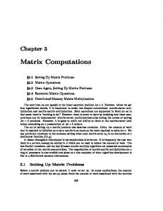
are shown in red. All these values in turn depend on the k = 8 leftmost value of x(0) owned by the right processor, shown as black circles containing red asterisks in the bottom row. By sending these values from the right processor to the left processor, the left processor can compute all the circles whose dependencies are shown in Figure 1(b). The black circles indicate computations ideally done only by the left processor, and the red circles show redundant computations, i.e., those also performed by the right processor. We assume that k < np , so that only data from neighboring processors is needed, rather than more distant processors. Indeed, we expect that k $ np in practice, which will mean that the number of extra flops (not to mention extra memory) will be negligible. We continue to make this assumption later without repeating it, and use it to simplify some expressions in Table 1. Figure 1(c) illustrates PA2. We note that the blue circles owned by the right processor and attached to blue lines can be computed locally by the right processor. The 8 circles containing red asterisks can then be sent to the left processor to compute the remaining circles connected to black and/or red lines. This saves the redundant work represented by the blue circles, but leaves the redundant work to compute the red circles, about half the redundant work of PA1. PA2 takes roughly 52 k 2 more flops than PA0, which is half as many extra flops as PA1.

3. Number of messages sent per processor (the “latency cost”); 4. Total memory required per processor for the matrix; and 5. Total memory required per processor for the vectors. Informally, it’s clear that both PA1 and P2 minimize communication to within a constant factor. We ignore cancellation in any of the Aj or Aj x, so that the complexity only depends on the sparsity pattern of A. For simplicity of notation we assume all the nonzero entries of A and x are positive. Then, the set D of processors owning entries of x on which block row i of [Ax,A2 x,. . . ,Ak x] depends is just the set of processors owning those xj for which block row i of A + A2 + · · · + Ak has a nonzero j-th column. In both algorithms PA1 and PA2, the processor owning row block i receives exactly one message from each processor in D, which minimizes latency. Furthermore, PA1 only sends those entries of x in each message on which the answer depends, which minimizes the bandwidth cost. PA2 sends the same amount of data although different values so as to minimize redundant computation.

3.1

1D meshes

We now illustrate the difference between PA0, PA1, and PA2, using the example of a 1D mesh with bandwidth b = 1, or a tridiagonal matrix. In PA0, the computational cost is 2k messages, 2k words sent, and 5k np flops (3 multiplies and 2 additions per vector component computed). The memory required per processor is 3 np matrix entries and (k + 1) np + 2 vector entries (for the local components of [x, Ax, .., Ak x] and for the values on neighboring processors). Figure 1(a) shows the operation of PA1 with k = 8. Each row of circles represents the entries of Aj x, for j = 0 to j = 8. A subset of 30 components of each vector is shown, owned by 2 processors, one to the left of the vertical green line, and one to the right. (There are further components and processors not shown.) The diagonal and vertical lines show the dependencies: the three lines below each circle (component i of Aj x) connect to the circles on which its value depends (components i − 1, i and i + 1 of Aj−1 x). In the figure, the local dependencies of the left processor are all the circles that can be computed without communicating with the right processor. The remaining circles without attached lines to the left of the vertical green line require information from the right processor before they can to be computed. Figure 1(b) shows how to compute these remaining circles using PA1. The dependencies are again shown by diagonal and vertical lines below each circle, but now dependencies on data formally owned by the right processor

3.2

Summary of Parallel Complexity of Computing [Ax, ..., Ak x] on Meshes

PA1 and PA2 can be extended to higher dimensions and different mesh bandwidths (and sparse matrices in general). There, the pictures of which regions are communicated and which are computed redundantly become more complicated, higher-dimensional polyhedra, but the essential algorithms remain the same. Table 1 in Section 3.2 summarizes all of the resulting costs for 1D, 2D, and 3D meshes. In Table 1 which shows the summary for Parallel Algorithms, “Mess” is the number of messages sent per processor, “Words” is the total size of these messages, “Flops” is the number of floating point operations, “MMem” is the amount of memory needed per processor for the matrix entries, and “VMem” is the amount of memory needed per processor for the vector entries. Lower order terms are sometimes omitted for clarity.

3.3

General Graphs

We now extend the approaches PA1 and PA2 to general sparse matrices. To do so we need some graph theoretic notation. It is natural to associate a directed graph 3


Local Dependencies for k=8 8

7

6

5

4

3

2

1

0 5

10

15

20

(a) Locally computable components.

Type (1) Remote Dependencies for k=8 8

7

7

6

6

5

5

4

4

3

3

2

2

1

1

0

0 10

15

20

(b) Remote dependencies in PA1.

30

Type (2) Remote Dependencies for k=8

8

5

25

25

30

5

10

15

20

(c) Remote dependencies in PA2.

25

30

Figure 1. Dependencies for PA1 and PA2 for computing [Ax, ..., A8 x] for tridiagonal matrix. (i)

with a square sparse matrix A, with one vertex for every row/column, and an edge from vertex i to vertex j if Aij %= 0, meaning that component i of y = Ax depends on component j of x. We build an analogous graph, essen(i) tially consisting of k copies of this basic graph: Let xj be the j-th component of x(i) = Ai · x(0) . We associate (i) a vertex with each xj for i = 0, ..., k and j = 1, ..., n (and use the same notation to name the vertex), and an edge (i+1) (i) from xj to xm when Ajm %= 0, and call this graph of n(k + 1) vertices G. (We will not need to construct all of G in practice, but using G makes it easy to describe our algorithms, in a fashion analogous to Figure 1.) We say that (i) i is the level of vertex xj . Each vertex will also have an affinity q, corresponding to the processor number where it (0) (1) (k) is stored; we assume all vertices xj , xj , ..., xj have the same affinity, depending only on j.

Gq to mean the subset with affinity q and level i. Let S be any subset of vertices of G. We let R(S) denote the set of vertices reachable by directed paths starting at vertices in S (so S ⊂ R(S)). We need R(S) to identify dependencies of sets of vertices on other vertices. We let R(S, m) denote vertices reachable by paths of length at most m starting at vertices in S. We write Rq (S), R(i) (S) (i) and Rq (S) as before to mean the subsets of R(S) with affinity q, level i, and both affinity q and level i, respectively. Next we need to identify the locally computable components, that processor q can com(0) pute given only the values in Gq . We denote the set of locally computable components by (i) Lq ≡ {x ∈ Gq : R(x) ⊂ Gq }. As before Lq will denote the vertices in Lq at level i. Finally, for PA2 we need to identify the minimal subset Bq,r of vertices (i.e. their values) that processor r needs to

We let Gq denote the subset of vertices of G with affinity q, G(i) to mean the subest of vertices of G with level i, and 4


Problem

2D mesh

Costs Mess Words Flops MMem VMem Mess Words

Conventional Approach 2k 2bk (4b + 1)k np (2b + 1) np (k + 1) np + 2b 8k n 4bk( p1/2 + b)

(2b + 1)2

Flops

(8b2 + 8b + 1)k np

1D mesh b≥1

2

pt stencil

2

MMem

(2b + 1)2 np

VMem

n (k + 1) np + 4b p1/2 +4b2 26k 2 n 6bk pn2/3 + 12b2 k p1/3 3 +O(b k) 3 (2(2b + 1)3 − 1)k np

Flops

stencil

(2b +

3

(2b + 1)3 np

MMem

3

VMem

2

(k + 1) np + 6b pn2/3 n ) +O(b2 p1/3

Parallel Approach 2 2 2bk 2 (4b + 1)(k np + bk2 ) n (2b + 1) p + bk(2b + 1) (k + 1) np + 2bk 8 n 4bk( p1/2 + 1.5bk)

(8b2 + 8b + 1)· 2 (k np

2

Mess Words

3D mesh (2b + 1)3 pt

Parallel Approach 1 2 2bk (4b + 1)(k np + bk2 ) (2b + 1) np + bk(4b + 2) (k + 1) np + 2bk 8 n 4bk( p1/2 + bk)

3

2

+ 2bk p1/2 + 43 b2 k3 ) 2 n 1)2 ( np + 4bk p1/2 + 4b2 k2 ) n n2 (k + 1) p + 4bk p1/2 2 2

+4b k 26 2 n 6bk pn2/3 + 12b2 k2 p1/3 3 3 +O(b k ) (2(2b + 1)3 − 1)· 2

n )) (k np + 3bk2 pn2/3 + O(b2 k3 p1/3 3 ( np

(8b2 + 8b + 1)·

n

(2b + 1)3 ·

2 n + 6bk pn2/3 + O(b2 k2 p1/3 )) 3 2 n n (k + 1) p + 6bk p2/3 n ) +O(b2 k2 p1/3

(2b

2 n (k np + bk2 p1/2 + b2 k 3 ) 2 n + 1)2 ( np + 2bk p1/2 + b2 k 2 ) n n2 (k + 1) p + 4bk p1/2 2 2

3

+6b k 26 2 n 6bk pn2/3 + 12b2 k2 p1/3 3 3 +O(b k ) (2(2b + 1)3 − 1)· 2

n )) (k np + 32 bk2 pn2/3 + O(b2 k3 p1/3 3 ( np

(2b + 1)3 · 2

n + 3bk pn2/3 + O(b2 k2 p1/3 )) 3

2

(k + 1) np + 6bk pn2/3 n ) +O(b2 k2 p1/3

Table 1. Summary Table for Parallel Algorithms (some lower order terms omitted) send processor q so that processor q can finish computing all its vertices Gq (eg the 8 circles containing red asterisks in Figure 3): We say that x ∈ Bq,r if and only if x ∈ Lr , and there is a path from some y ∈ Gq to x such that x is the first vertex of the path in Lr . Given all this notation, we can finally state versions of PA0, PA1 and PA2 for general graphs and partitions among processors: PA0 (Code for proc. q) PA1 (Code for proc. q) for i = 1 to k do for all procs r = ! q do (i−1) send all xj (i−1)

(i)

(i−1)

(i)

in

Rq (Gr ) to proc. r for all procs r != q do (i−1) receive all xj in Rr (Gq ) from proc. r (i) (i) compute all xj in Lq wait for receives to finish (i) compute remaining xj in (i)

(i)

Gq − Lq

plicity we use a symmetric matrix so the edges can be undirected. The dotted orange lines separate vertices owned by different processors. We let q denote the processor owning the 9 gray vertices in the center of the figure. In other (0) words, the gray vertices are Gq . For all the neighboring (0) processors r %= q, the red vertices are Rr (Gq ) for k = 1, (0) the red and green vertices together are Rr (Gq ) for k = 2, (0) and the red, green and blue vertices together are Rr (Gq ) for k = 3.

for all procs r != q do (0) (0) send all xj in Rq (Gr ) to proc. r for all procs r != q do (0) (0) recv. all xj in Rr (Gq ) from proc. r for i = 1 to k do (i) compute all xj in Lq // ex: circled vertices in Figure 1(a) wait for receives to finish for i = 1 to k do (i) compute remaining xj in R(Gq ) − Lq // ex: circled vertices in Figure 1(b)

PA2 (Code for proc. q)

for i = 1 to k do // Phase I (i) compute xj in ∪r"=q (R(Gr ) ∩ Lq ) // ex: blue circled vertices in Figure 1(c) for all procs r != q do (i) send xj in Br,q to proc. r // blue circled vertices containing red asterisks in Figure 1(c) for all procs r != q do (i) recv. xj in Br,q from proc. r // blue circled vertices containing red asterisks in Figure 1(c) for i = 1 to k do // Phase II (i) compute xj in Lq − ∪r"=q (R(Gr ) ∩ Lq ) // ex: locally computable vertices of right proc. minus blue circled vertices in Figure 1(c) wait for receives to finish for i = 1 to k do // Phase III (i) compute remaining xj in R(Gq ) − Lq − ∪r"=q (R(Gq ) ∩ Lr ) // ex: black circled vertices in Figure 1(c) that are connected by lines

We illustrate the algorithm PA1 on the matrix A whose graph is in Figure 2(a). The vertices represent rows and columns of A and the edges represent nonzeros; for sim5


5

The Phases in PA2 are referred to in Section 6. Figures 2(b) and 2(c) illustrate algorithm PA2 on the same matrix (as the one used for PA1), just for the case k = 3. In (0) Figure 2(b), the red vertices are Bq,r (the members of Bq,r (1) at level 0), and in Figure 2(c) the green vertices are Bq,r .

4

Asymptotic Performance

An asymptotic performance model for the parallel algorithms suggests that when the latency α is large, the speedup is close to k as expected (Section 4, [5]). When α is not so large, the best we could hope for is that k can be chosen so that the new running time is fast independent of α. The model shows that this is the case under two reasonable conditions:

Sequential Algorithms

We briefly describe two sequential algorithms, both of which emulate the parallel algorithm PA1 (Section 3.3):

1. The time it takes to send the entire local contents of a processor is dominated by bandwidth, not latency, and

• Conventional Sequential Approach (SA0): We assume that the matrix does not fit in fast memory but the vectors do. This algorithm will keep all the components of [x, Ax, . . . , Ak x] in fast memory, and read all the entries of A from slow to fast memory to compute each vector Aj x, thereby reading A k times in all.

2. The time to do O(N 1/d ) flops on each of the N elements stored on a processor exceeds α. For the sequential algorithm SA2, if latency is small enough, then the asymptotic performance model suggests the following: 1. The best speedup is bounded by 2 + (words/row), where words/row is the number of 8-byte words per row of the matrix A–this includes the index entries too.

• Sequential Approach 1 (SA1): We assume that the matrix does not fit in fast memory but the vectors do. SA1 emulates PA1 by partitioning the matrix into p block rows, and looping from i = 1 to i = p, reading from slow memory those parts of the matrix needed to perform the same computations performed by processor i in PA1, and updating the appropriate components of [Ax, . . . , Ak x] in fast memory. Since all components of [Ax, . . . , Ak x] are in fast memory, no redundant computation is necessary. We choose p as small as possible, to minimize the number of slow memory accesses.

2. The optimal speedup is strongly dependent on the β/tf ratio. For the specific case of stencils, the optimal speedup is expected to be close to the upper bound in the previous item when β/tf is large.

6

Detailed Performance Modeling

In this section we present detailed performance models of matrices with 2D ((2b + 1)2 -point) and 3D ((2b + 1)3 point) stencil graphs for PA2 and SA2 using realistic machine parameters, in order to identify situations where significant speedups are likely. We assume that we can overlap communication and computation for the parallel algorithms. Although these are stencil graphs, we assume general sparse matrix storage, because our algorithms apply to general sparse matrices. As before, we assume that quantin ties like p1/2 and p1/3 are integers. We model PA2 for two parallel machines called Peta (which is a model of a nominal 8100 processor petascale machine) and Grid (which is a model of 125 terascale machines connected over the internet). The two sequential machines for which we model SA2 are OOC (which models an out-of-core implementation, where fast memory is DRAM and slow memory is disk) and Clovertown (we call the model “CacheBlocked”), the Intel multicore processor (where fast memory is cache and slow memory is DRAM). This variety of models of course suggests that our techniques can be applied more than once, if there are several levels of memory hierarchy and possibly also parallelism.

• Sequential Approach 2 (SA2): Now we assume that neither the matrix nor the vectors fit in memory. SA2 will still emulate PA1 by looping from i = 1 to i = p, but read from slow memory not just parts of the matrix but also those parts of the vectors needed to perform the same computations performed by processor i in PA1, and finally writing back to slow memory the corresponding components of [Ax, . . . , Ak x]. Depending on the structure of A, redundant computation may or may not be necessary. We again choose p as small as possible. An interesting problem that occurs in SA2 is when parts of x are needed from slow memory, they might not be contiguously placed. Thus, entries of the vector x and the matrix A may be reordered to minimize slow memory communication cost. One formulation of this reordering Problem can be posed as a Travelling Salesman problem (Section 3.5, [5]). 6


(a) PA1 example: Red entries of x(0) are the ones needed when k = 1, green are the additional ones needed when k = 2 and blue are the additional ones needed when k = 3.

(b) PA2 example (k = 3): Entries of x(0) which need to be fetched are colored red.

(c) PA2 example (k = 3): Entries of x(1) which need to be fetched are colored green.

Figure 2. Example for PA1 and PA2. The dotted lines define the different blocks. Each block resides on a different processor. The example shows from the perspective of the processor holding the central block.

6.1

Performance Modeling of PA2

Note that each processor in Peta and Grid is a significant parallel computer itself, but we only model the parallelism between these processors, not within them. Again, one could potentially apply our techniques for each level of parallelism, but we have not modeled this here. In Section 3.3 we described the three computational phases of PA2: Phase I must be done before any communication can be initiated, Phase II can be fully overlapped with communication, and Phase III can only begin after communication is complete. This justifies the performance model below, given the assumption of overlapping communication. Let NI , NII , and NIII respectively denote the flop counts for Phases I, II, and III of PA2–the formulas for these are shown in Table 6.1. Let Nw denote the total number of words sent by a processor. Let M denote the memory required per processor when p processors are used. Formulas for Nw and M are only slightly more detailed than the entries in Table I, so we do not show them here. Let Tk,p denote the time taken for PA2. Since we assume all messages can be in-flight simultaneously while computation is occurring. So, we use Tk,p = (NI + NIII ) · tf + max (NII · tf , α + β · Nw ). For performance modeling, we find the optimal value of the parameter p within the range allowed for specific n, k, b values. This range is limited by two parameters–pmax and mem. If p is made small, then the memory required per processor M might exceed the memory available per processor mem. Also, p can be at most pmax . Another limit imposed on p is that the number of entries per dimension of the stencil should be be at least 2bk since our formulas assume this condition. We also round p down to the

We consider parallel machines with the following parameters: pmax : The maximum number of processors available. The actual number of processors used is p ≤ pmax . We may choose p < pmax if that is faster. tf : The time per floating-point operation (in units of seconds), modeled as 10% of machine peak value, a typical value attainable for SpMV. mem: The memory available per processor (in units of 8-byte words). α: The network processor latency (in units of seconds). β: The inverse network bandwidth (in units of seconds/8byte word). Thus the time to send m words between any pair of processors is modeled as α + βm. We modeled machines with the following parameter values: Peta: pmax = 8100, tf = 2 · 10−11 secs (1/tf = 50 GFlops/s), mem = 62.5 · 109 words, α = 10−5 secs, β = 2 · 10−9 secs (1/β = 500 MWords/s = 4 GByte/s) Grid: pmax = 125, tf = 10−12 secs (1/tf = 1T F lop/s), mem = 1.2·1012 words, α = 10−1 secs, β = 25·10−9 secs (1/β = 40 MWords/s = .32 GBytes/s) (estimated by dividing the Teragrid backbone bandwidth of 40 GBytes/s by pmax .) 7


Problem

Term NI

2D

NII NIII NI

3D

NII NIII

“Formula ” n (8b2 + 8b + 1) · − bk · (bk2 − 2bk) “ 2 p1/2 ” 3n 9bkn 2 (8b + 8b + 1) · − 1/2 + 7b2 k2 + 2b2 · k/3 p “p ” (8b2 + 8b + 1) · bk · 9nk + 6n − bk2 − 6bk − 8b /3 1/2 1/2 p “ p2 ” 12bkn 2 2 2 (2(2b + 1)3 − 1) · (bk2 − 2bk) · 6n 2/3 − p1/3 + 7b k − 2b k /4 p “ 3 ” 2 (28b2 k2 +8b2 )n (2(2b + 1)3 − 1) · k · 4n − 18bkn + + O(b3 k3 ) /4 2/3 1/3 p p p “ 2 ” 2 2 3 (2(2b + 1)3 − 1) · bk · n2/3 (18k + 12) − nb 1/3 (4k + 24k + 32) + O(b k ) /4 p

p

Table 2. Formulas for NI , NII and NIII for PA2. nearest perfect square or cube (depending on the problem). The optimal p is strongly problem dependent, e.g., for small problem sizes, p = 1 might be sufficient and better since it avoids the overhead of communication. Therefore, a good measure of how well PA2 performs with respect to the conventional algorithm is the speedup with respect to the conventional algorithm assuming optimal p values were used min max T1,p ·k for each algorithm: speedup = min1≤p≤p . We 1≤p≤pmax Tk,p used T1,p · k for the time taken for the conventional algorithm as the conventional algorithm turns out to be k invocations of PA2 with k = 1. We now discuss the performance modeling results for each combination of machine (Peta or Grid) and stencil (2D or 3D with bandwidth b = 1):

new algorithm (with the exception of a 2% speedup for n = 29 and k = 2). This is because the conventional k = 1 algorithm is already completely dominated by computation. 4. 3D Stencil on Grid (Figure 3(d)): In this case we can get a speedup of 4.41x for n = 210 and k = 30.

6.2

Performance Modeling of SA2

Here, we present a brief summary of the detailed performance modeling of the sequential algorithm SA2. We modeled two machines with the following parameters: 1. OOC: This out-of-core implementation models a 500 MFlop/s uniprocessor with 4 GB DRAM as fast memory and a 15000 RPM Seagate ST373307 disk as slow memory. The disk access latency is 5.7 ms and bandwidth is 62.5 MB/s.

1. 2D Stencil on Peta (Figure 3(a)): We see that for smaller n and k, the speedup is close to linear in k. The best speedup is 6.9x, attained when n = 211 , k = 12. However, the algorithm has no benefit for large values of n, because computation totally dominates communication; in this case no optimization is necessary either. We also note that the speedup decreases as k is increased beyond a certain point, because the overhead of extra floating point operations exceeds the gains from reducing latency.

2. CacheBlocked: This implementation models a single core of the quad-core Intel Clovertown chip, with 2 GFlops/s (based on measurements in [27]) with onchip 8 MB cache as fast memory and DRAM as slow memory. The DRAM access latency is 200 ns and bandwidth is 5 GB/s. The performance of SA2 was modeled for the specific case of 2D 9-point stencil and 3D 27-point stencil as the matrix A. Our model assumes no overlap of communication with computation, in order to compare with our implementation. Table 3 shows the predicted speedups: In contrast to the parallel case, we see that significant speedups were attained for all problem sizes n, since bandwidth is always the bottleneck. In the table, “% Peak” is the ratio of the (modeled) running time of the algorithm on a zero latency / infinite bandwidth machine to the (modeled) true time. The closer this is to 100%, the more completely the algorithm masks the cost of slow memory access. On OOC, we see that we get high speedups, though we are not near peak performance. On CacheBlocked, our speedups are more modest, but still good, and we are closer to peak performance.

2. 2D Stencil on Grid (Figure 3(b)): The white region for n = 221 and n = 222 indicates that the problem needed too much memory to be solved by the machine. We see that the algorithm is expected to obtain an impressive speedup of up to 22.22x for large matrices (n = 217 ). Indeed, speedup is still increasing for the maximum value of k shown (k = 30), and larger k might show further improvements. No speedups are expected for small values of n because the problem can be solved using only 1 processor and latency is too high to benefit from using more processors. As before, for very large problem sizes (n ≥ 220 ), we see no gains because computation dominates communication. 3. 3D Stencil on Peta (Figure 3(c)): In contrast to the 2D case, in the 3D case no speedup is possible using our 8


(a) Peta: Speedup for 2D stencil

(b) Grid: Speedup for 2D stencil

(c) Peta: Speedup for 3D stencil

(d) Grid: Speedup for 3D stencil

Figure 3. Performance modeling plots for Peta and Grid. Model OOC CacheBlocked

Matrix 2D 3D 2D 3D

Range of n 214 to 225 28 to 217 28 to 219 28 to 212

(Range of) Modeled Speedup 10.2 [7.39,9.51] [2.45,2.58] [1.34,1.36]

(Range of) % Peak 17% [14%, 18%] [62%, 65%] 38%

Table 3. Performance modeling summary for SA2.

7

Measured Performance

NERSC Jacquard cluster2 (AMD Opteron-based). However, since the network for these machines has low latency, there were no speedups from our parallel algorithms. Our sequential implementation, however, shows good speedups. So, we report the performance results for our implementation of SA2. For the implementation of SA2, we needed to solve

We implemented PA1 and PA2 for general sparse matrices in UPC [8]. We tested our implementation on the UC Berkeley CITRIS cluster1 (Intel Itanium 2-based) and the 1 The authors wish to acknowledge the contribution from Intel Corporation, Hewlett-Packard Corporation, IBM Corporation, and the National Science Foundation grant EIA-0303575 in making hardware and software available for the CITRIS Cluster which was used in producing these research results.

2 This research used resources of the National Energy Research Scientific Computing Center, which is supported by the Office of Science of the U.S. Department of Energy under Contract No. DE-AC02-05CH11231.

9


8

an ordering problem for the rows of x and A in order to minimize the communication cost (Section 4). This minimization problem corresponds to minimizing the number of words fetched from disk during the course of the algorithm. We used a simple random sampling strategy to choose the best ordering from a sequence of random orderings. This worked out well as the actual number of words transferred between disk and main memory was close to the lower bound for SA2 (within 2%). Another level of reordering was done on a per-block basis in our implementation. This allowed the computations in SA2 to be done as a sequence of k calls to separate, tuned sparse matrix multiplication (SpMV) routines. In our implementation we used the OSKI library [26]. We tested our implementation on the UC Berkeley CITRIS cluster–a cluster of Itanium 2 nodes each with a theoretical peak performance of 5.2 GFlops/s. Each node has 2 Itanium processors with 4 gigabytes of memory per processor. Our test problem was a matrix with a 27-point stencil on a 3D mesh (stored as a general sparse matrix) with n = 368 and p = 64 (the choice of n was limited by the available disk space). Thus the matrix had dimension 3683 = 49, 836, 032 with 27 nonzeros in most rows, bro3 3 ken into 43 = 64 blocks of ( 368 4 ) = 92 = 778, 688 rows each. The value of p was chosen to optimize performance. For accurate performance modeling, we used measured values for all important machine parameters: time per floating point operation and disk bandwidth. The disk bandwidth differs significantly for reads and writes, so we augmented our model to distinguish reads and writes. Disk latency turned out to play a negligible role.

Related Work

The optimizations described in this paper belong to a collection of techniques for improving the performance of applying a stencil repeatedly to a regular discrete domain, or multiplying a vector repeatedly by a sparse matrix. They, in turn, are a subset of various methods known as tiling or blocking. They all involve decompositions of the ddimensional domain into d-dimensional subdomains, and rearranging the order of arithmetic operations in order to exploit the parallelism and/or temporal locality implicit in those subdomains. Tiling research falls into three general categories. The first encompasses performance-oriented implementations and practical performance models. See, for example, [17, 16, 10, 28, 18, 14, 21, 29, 7, 22, 6, 30, 25, 12, 11]. The second category consists of theoretical algorithms and asymptotic performance analyses. These are based on sequential or parallel processing models which account for the memory hierarchy and/or inter-processor communication costs. Works that specifically discuss stencils or more general sparse matrices include [9], [13], and [23]. The third category contains suggested applications that call for repeated application of a stencil (resp. sparse matrix) to a domain (resp. vector). See, for example, [24, 19, 2, 3, 1, 22]. The idea of using redundant computation to avoid communication or slow memory accesses in stencil codes may be as old as OOC stencil codes themselves. Leiserson et al. cite a reference from 1963 [13, 17]. Nevertheless, many tilings do not involve redundant computation. For example, Douglas et al. describe a parallel tiling algorithm that works on the interiors of the tiles in parallel, and then finishes the boundaries sequentially [7]. Many sequential tilings do not require redundant computations [11]; our SA1 algorithm does not. However, at least in the parallel case, tilings with redundant computation have the advantage of requiring only a single round of messages, if the stencil is applied several times. The latency penalty is thus independent of the number of applications, though the bandwidth requirements increase. Furthermore, Strout et al. point out that the sequential fill-in of boundary regions suggested by Douglas et al. suffers from poor locality [22]. Most importantly, redundant computation to save messages is becoming more and more acceptable, given the exponential divergence in performance between latency, bandwidth, and floating-point rate. Extensions of stencil tiling to more general sparse matrices require runtime analysis of the sparse matrix structure, often using a graph partitioner. Finding an optimal partition is an NP-complete problem which must be approximated in practice, at nontrivial cost. Theoretical algorithms for the out-of-core sequential case already existed (see e.g., [13]),

• tf = 3.12 ns (1/tf = 321 Mflops/s): This is the measured inverse flop rate for SA2. This was taken as the median of the flop rates observed for the computational phases in SA2. • βr = 56 ns (1/βr = 143 MBytes/s): This is the measured inverse read bandwidth. • βw = 240 ns (1/βw = 33 MBytes/s): This is the measured inverse write bandwidth. Figures 4(a) and 4(b) show the results, both modeled and measured, which closely match. Figure 4(a) breaks the total runtime down into computation and communication, and Figure 4(b) shows the speedup, which reaches 3.2x at k = 15, and is at least 3x for k ≥ 8. We also compare the results to those on a hypothetical machine with infinite DRAM, so that the the entire computation can proceed in main memory. Such an algorithm obviously provides an upper bound on our speed. We go from running 20x slower than this algorithm at k = 1 to just 6x slower at k = 15 (these are measured values). 10


(a) Measured vs. Modeled SA2 Performance.

(b) Measured vs. Modeled SA2 speedup.

Figure 4. Measured performance plots for SA2 on Itanium2 CITRIS cluster. entirely in fast memory. As far as we can tell, PA2 and SA2 are novel.

but Douglas et al. were apparently the first to attempt an implementation of parallel tiling of a general sparse matrix, in the context of repeated applications of a multigrid smoother [7]. This was extended by Strout et al. into a sequential cache optimization which resembles our SA1 algorithm. Our work differs from existing approaches in many ways. First, we developed our methods in tandem with an algorithmic justification: communication-avoiding or “sstep” Krylov subspace methods [4]. Toledo had suggested an s-step variant of conjugate gradient iteration, based on a generalization of PA1, but he did not supply an implementation for matrices more general than tridiagonal matrices [23]. We have a full implementation of PA1 for general sparse matrices, and have detailed theoretical models showing performance increases on a wide variety of platforms. Douglas et al. and Strout developed their matrix powers kernel for classical iterations like Gauss-Seidel [7, 22]. However, these iterations’ most common use in modern linear solvers are as multigrid smoothers. The payoff of applying a smoother k times in a row decreases rapidly with k; this is, in fact, why multigrid is used, rather than classical iterations such as Jacobi or Gauss-Seidel. Douglas et al. acknowledge that usually 1 ≤ k ≤ 5 [7]. In contrast, communication-avoiding Krylov subspace methods are potentially much more scalable in k. Saad also suggested applying something like a matrix powers kernel to polynomial preconditioning, but here again, increasing the degree of the polynomial preconditioner has a decreasing payoff, in terms of the number of CG iterations required for convergence [19]. We have also expanded the space of possible algorithms by including PA2 and SA2. PA2 avoids some redundant computation, but offers less opportunity for overlapping communication and computation. SA2 extends SA1 for the case in which the vectors (as well as the matrix) do not fit

9

Conclusions

To address both current and future gaps between computational speed and communication speed, we are developing a set of communication avoiding algorithms to minimize data movement within local memory hierarchies and between processors. In this paper we presented both serial and parallel algorithms for the matrix powers kernel, which can be used in place of individual sparse matrix vector multiplication in Krylov Subspace Methods and elsewhere. The powers kernel amortizes the bandwidth cost of reading the matrix A by breaking A into blocks that fit in a single processor or a fast memory system and taking multiple steps on those blocks. We present algorithms with minimal communication costs, which send a single message (or slow matrix read) for k matrix-vector products computed in the matrix powers kernel, compared to k such operations in the conventional approach. We also show variations of the algorithms that trade off communication cost for redundant work. Our algorithms are of practical as well as theoretical interest. We developed detailed performance models for both serial and parallel algorithms, instantiating the parallel model with parameters that are expected to be typical for a Petascale machine and for computing across the Grid. The serial model is instantiated with numbers from a current processor memory hierarchy and for an out-of-core setting. Our detailed performance model predicts more than 4x speedups for high latency parallel machines (Grid) for moderate sized stencils. In the sequential case, our proposed algorithm avoids both latency and bandwidth (in contrast to the parallel machine, where only latency is avoided), which 11


gives speedups for all problem sizes. The performance of our sequential implementation is promising indeed, with speedups of 3x over the conventional algorithm. In addition to the specific results in this paper, we believe this work reflects a shift in algorithm design that will be necessary for future systems; this approach carefully counts communication costs and may favor algorithms with higher computational cost if they avoid communication.

[14]

[15] [16]

References [17] [1] Z. Bai, D. Hu, and L. Reichtel. A Newton basis GMRES implementation. IMA Journal of Numerical Analysis, 14:563– 581, 1994. [2] A. T. Chronopoulos and C. W. Gear. s-step iterative methods for symmetric linear systems. J. Comput. Appl. Math., 25(2):153–168, 1989. [3] E. de Sturler. A parallel variant of GMRES(m). In J. J. H. Miller and R. Vichnevetsky, editors, Proc. of the 13th IMACS World Congress on Computation and Applied Mathematics, Dublin, Ireland, 1991. Criterion Press. [4] J. Demmel and M. Hoemmen. Communication-avoiding variants of gmres and cg. Technical Report in preparation, Computer Science Department, University of California Berkeley, 2007. [5] J. Demmel, M. Hoemmen, M. Mohiyuddin, and K. Yelick. Avoiding communication in computing Krylov subspaces. Technical Report UCB/EECS-2007-123, Computer Science Department, University of California Berkeley, 2007. [6] C. Ding and Y. He. A ghost cell expansion method for reducing communications in solving PDE problems. In Proc. of SC01, Nov. 2001. [7] C. C. Douglas, J. Hu, M. Kowarschik, U. R¨ude, and C. Weiss. Cache optimization for structured and unstructured grid multigrid. Electronic Transaction on Numerical Analysis, 10:21–40, Feb. 2000. [8] T. El-Ghazawi, W. Carlson, T. Sterling, and K. Yelick. UPC: Distributed Shared-Memory Programming. WileyInterscience, May 2005. [9] J.-W. Hong and H. T. Kung. I/O complexity: The red-blue pebble game. In Proc. 13th Ann. ACM Symp. on Theory of Computing (May 11-13, 1981), pages 326–333, 1981. [10] F. Irigoin and R. Triolet. Supernode partitioning. In Proc. of the 15th ACM SIGPLAN-SIGACT Symp. on Principles of Programming Languages, pages 319–329. ACM Press, 1988. [11] S. Kamil, K. Datta, S. Williams, L. Oliker, J. Shalf, and K. Yelick. Implicit and explicit optimizations for stencil computations. In Memory Systems Performance and Correctness, San Jose, CA, Oct. 2006. [12] S. Kamil, P. Husbands, L. Oliker, J. Shalf, and K. Yelick. Impact of modern memory subsystems on cache optimizations for stencil computations. In 3rd Ann. ACM SIGPLAN Workshop on Memory Systems Performance, Chicago, IL, 2005. [13] C. E. Leiserson, S. Rao, and S. Toledo. Efficient out-ofcore algorithms for linear relaxation using blocking covers

[18] [19] [20] [21]

[22]

[23]

[24] [25] [26]

[27]

[28] [29]

[30]

(extended abstract). In IEEE Symp. on Foundations of Computer Science, pages 704–713, 1993. J. McCalpin and D. Wonnacott. Time skewing: A valuebased approach to optimizing for memory locality. Technical Report DCS-TR-379, Department of Computer Science, Rutgers University, 1999. D. Patterson. Latency lags bandwidth. CACM, 47(10):71– 75, Oct 2004. J.-K. Peir. Program partitioning and synchronization on multiprocessor systems. PhD thesis, Department of Computer Science, University of Illinois at Urbana-Champaign, Mar. 1986. C. J. Pfeifer. Data flow and storage allocation for the PDQ-5 program on the Philco-2000. Communications of the ACM, 6(7):365–366, 1963. E. J. Rosser. Fine-grained analysis of array computations. PhD thesis, Dept. of Computer Science, University of Maryland, Sept. 1998. Y. Saad. Practical use of polynomial preconditionings for the conjugate gradient method. SIAM J. Sci. Stat. Comput., 6(4), Oct. 1985. M. Snir and S. Graham, editors. Getting up to speed: The Future of Supercomputing. National Research Council, 2004. 227 pages. Y. Song and Z. Li. New tiling techniques to improve cache temporal locality. In Proc. ACM SIGPLAN Conference on Programming Language Design and Implementation, Atlanta, GA, 1999. M. M. Strout, L. Carter, and J. Ferrante. Rescheduling for locality in sparse matrix computations. In V. N. Alexandrov and J. J. Dongarra, editors, Lecture Notes in Computer Science. Springer, 2001. S. Toledo. Quantitative performance modeling of scientific computations and creating locality in numerical algorithms. PhD thesis, Massachusetts Institute of Technology, June 1995. J. van Rosendale. Minimizing inner product data dependence in conjugate gradient iteration. In Proc. IEEE Internat. Confer. Parallel Processing, 1983. R. Vuduc. Automatic Performance Tuning of Sparse Matrix Kernels. PhD thesis, University of California Berkeley, Dec. 2003. R. Vuduc, J. Demmel, and K. Yelick. OSKI: A library of automatically tuned sparse matrix kernels. In Proc. of SciDAC 2005, J. of Physics: Conference Series. Institute of Physics Publishing, June 2005. S. Williams, L. Oliker, R. Vuduc, J. Shalf, K. Yelick, and J. Demmel. Optimization of sparse matrix-vector multiplication on emerging multicore platforms. In SC07. IEEE, 2007. to appear. M. E. Wolf. Improving locality and parallelism in nested loops. PhD thesis, Stanford University, 1992. D. Wonnacott. Using time skewing to eliminate idle time due to memory bandwidth and network limitations. In Proc. of the 14th Int. Parallel and Distributed Processing Symp. (IPDPS), pages 171–180, 2000. P. R. Woodward and S. E. Anderson. Scaling the Teragrid by latency tolerant application design. In Proc. of NSF / Department of Energy Scaling Workshop, Pittsburg, CA, May 2002.

12
