Nov 20, 2009 - rithm just for a single sparse matrix-vector multiplication (SpMV, or A · x). ... Convergence analysis for a variety of practical matrices shows that the new algorithm ... (for convergence rate) independently. ..... to introduce additional notation. We now ...... scientific computations and creating locality in numerical.
Minimizing Communication in Sparse Matrix Solvers Marghoob Mohiyuddin∗†, Mark Hoemmen∗, James Demmel∗, Katherine Yelick∗† ∗ EECS Department, University of California at Berkeley, CA 94720, USA CRD/NERSC, Lawrence Berkeley National Laboratory, Berkeley, CA 94720, USA
†
ABSTRACT Data communication within the memory system of a single processor node and between multiple nodes in a system is the bottleneck in many iterative sparse matrix solvers like CG and GMRES. Here k iterations of a conventional implementation perform k sparse-matrix-vector-multiplications and Ω(k) vector operations like dot products, resulting in communication that grows by a factor of Ω(k) in both the memory and network. By reorganizing the sparse-matrix kernel to compute a set of matrix-vector products at once and reorganizing the rest of the algorithm accordingly, we can perform k iterations by sending O(log P ) messages instead of O(k · log P ) messages on a parallel machine, and reading the matrix A from DRAM to cache just once, instead of k times on a sequential machine. This reduces communication to the minimum possible. We combine these techniques to form a new variant of GMRES. Our shared-memory implementation on an 8-core Intel Clovertown gets speedups of up to 4.3× over standard GMRES, without sacrificing convergence rate or numerical stability.
1.
INTRODUCTION
The costs of arithmetic and communication continue to decrease, where “communication” means moving data, either between fast and slow memory (e.g., cache and DRAM) in the sequential case, or between processors over a network in the parallel case. However, arithmetic is getting faster much more quickly than communication, so that the primary challenge is developing algorithms to avoid communication. This is especially true in sparse matrix computations, where conventional algorithms do only a few arithmetic operations per datum, so that communication costs frequently dominate already. In this paper we show how to eliminate most of the communication from GMRES [20], a widely used iterative solver for sparse systems of equations Ax = b. Like other so-called Krylov Subspace Methods (KSMs), GMRES takes a starting vector (say v0 = b), creates a sequence of vectors v1 , . . . , vk where each vi is gotten by multiplying some linear combination of v0 , . . . , vi−1 by A, and then chooses the “best” (in some sense) approximate solution to Ax = b from the subspace of all linear combinations of v0 ,
(c) 2009 Association for Computing Machinery. ACM acknowledges that this contribution was authored or co-authored by a contractor or affiliate of the [U.S.] Government. As such, the Government retains a nonexclusive, royalty-free right to publish or reproduce this article, or to allow others to do so, for Government purposes only. SC09 November 14-20, 2009, Portland, Oregon, USA Copyright 2009 ACM 978-1-60558-744-8/09/11 ...$10.00.
. . . , vk (the Krylov subspace). This means that the cost in arithmetic and communication of GMRES (or any KSM) grows by a factor of Ω(k). (In fact, for conventional GMRES without restarting, the number of BLAS1 or BLAS2 flops grows proportionally with Ω(k2 ) for k iterations, and k sparse matrix-vector products are required besides.) In this paper we show how to reduce the communication cost of k iterations of GMRES by a factor of O(k), which is optimal, without sacrificing numerical stability or the convergence rate. In the parallel case with P processors, we decrease the latency cost (total number of messages) to Θ(log P ) from Ω(k log P ), and in the sequential case, we decrease the bandwidth cost (total numbers of words moved) by a factor of Ω(k). This requires several algorithmic innovations. Section 2 discusses our new matrix powers kernel W = [p0 (A) · b, p1 (A) · Q b, . . . , pk (A) · b], where pi (A) = ij=1 (A − λj · I) is a degreei polynomial in A, and the λi are constants chosen as described in Section 4 to improve numerical stability of the entire iterative method. This is a modification to the kernel defined in [8,9], namely [Ax, A2 x, . . . , Ak x]. Using ideas previously introduced in [8, 9], we describe how to compute W for the same bandwidth cost as 1 + o(1) sparse matrix-vector multiplies, and for about the same latency costs as a single matrix-vector multiply. Performance data on an 8-core 2.33 GHz Intel Clovertown shows speedups for computing W of up to 2.7× over k calls to the best optimized algorithm just for a single sparse matrix-vector multiplication (SpMV, or A · x). The columns of W span the same Krylov subspace as the vectors originally computed by GMRES, but GMRES must be reformulated to compute the best linear combination of these new basis vectors. Part of this reformulation is described in Section 3, where a communication-avoiding QR factorization of W is discussed; this was introduced in [5]. Performance data shows significant speedups over both Modified Gram-Schmidt orthogonalization and LAPACK’s Householder-based QR, both as a standalone factorization and as a way to orthogonalize the Arnoldi basis vectors in our version of GMRES. Section 4 discusses the overall reformulation of GMRES, which we call Communication-Avoiding GMRES (CA-GMRES). CAGMRES is equivalent to standard GMRES in exact arithmetic. Convergence analysis for a variety of practical matrices shows that the new algorithm converges at the same rate as standard GMRES. Overall measured performance results are in Section 4.5, which show speedups of up to 4.3× over conventional GMRES using the best available parallel SpMV. Finally, Section 5 discusses conclusions and future work. To summarize, our contributions in this paper include, first, autotuned and cotuned multicore implementations of two kernels (ma-
trix powers and TSQR) already introduced in earlier publications. Second, it describes a full implementation of the GMRES solver based on the aforementioned kernels. Finally, this solver has the ability to choose the matrix powers basis length k (for numerical stability and kernel performance) and the restart length m = k · t (for convergence rate) independently. Previous work was restricted to m = k. Thus, in order to avoid catastrophic failure due to numerical instability, earlier methods had to choose a short restart length m. However, this made them converge more slowly than our methods, or not at all.
2.
THE MATRIX POWERS KERNEL
As mentioned above, the matrix powers kernel takes a sparse matrix A, a dense vector x, and scalars λ1 , . . . , λk (chosen as described in Section 4), and computes the vectors (A − λ1 I)x, (A − λ2 I)(A − λ1 I)x, . . . , (A − λk I)(A − λk−1 I) · · · (A − λ1 I)x. Note that this is a slight modification to the kernel defined in [9], namely [Ax, A2 x, . . . , Ak x]. From an implementation perspective, the kernels differ only slightly from each other, and we refer to both by the same name. A naïve algorithm for our new kernel would proceed as follows: compute x0 = (A − λ1 I)x, then use x0 to compute x00 = (A − λ2 I)x0 , and so on. This is the same as k calls to sparsematrix vector multiplication (SpMV), which is a memory bound kernel and fails to exploit potential reuse of the matrix A. The algorithms we described in [8] for the matrix powers kernel reduce the slow memory traffic to the minimum possible – that is, they read the matrix A only once (with some overhead). While work in [9] focused on a sequential out-of-core implementation, where the gap between bandwidth and computational capability is especially large, this paper demonstrates that significant improvements are possible even for a multicore out-of-cache implementation. We note that our parallel, distributed-memory implementation in [9] had no performance improvements, because it lacked singlenode optimizations. In contrast, a multiple-node implementation built using our multicore out-of-cache implementation presented in this paper is expected to achieve significant performance improvements. We will, however, leave this multinode implementation as future work. To motivate our algorithms, we consider the simple case when the matrix A is tridiagonal (the dependency graph of the vectors (i) is shown in Figure 1). Let xj be the j-th component of x(i) = (A − λi I) · · · (A − λ1 I)x(0) . Although not shown throughout the figure, each entry depends on the one below it and its two neigh(0) (0) (0) (1) bors, e.g., x5 depends on x4 , x5 and x6 as shown by purple arrows in Figure 1. The vectors and the rows of the matrix are partitioned into p = 4 blocks. In the parallel algorithm, each block resides on a different processor and in case of a sequential algorithm, the blocks are computed one at a time. Consider the green colored block in Figure 1(a). For the parallel algorithm, if one processor has the entries of x(0) numbered from 18 to 33 (the base of the third trapezoid), then we can compute all the green entries – the non-green entries will need to be explicitly fetched from other blocks. Thus, instead of fetching non-green entries for every x(i) , we fetch them only once, which improves performance by reducing the number of inter-processor messages. However, we will be computing extra entries, which do not reside on the green partition, e.g., entries 19, 20, 31, 32 of x(1) – this constitutes redundant computation. The explicit sequential algorithm emulates the parallel algorithm by iterating over blocks (each block fits in fast memory) and computing on a block in the same manner as the parallel algorithm. In the explicit sequential algorithm, the benefits are even
more significant, because we are reading the matrix A from slow memory just a little more than once. However, because we perform redundant flops, some of the entries of A are fetched more than once from slow memory. If the number of redundant flops is small, we are effectively reading the matrix only once, whereas the naïve strategy would have read the matrix k times, which translates to a potential speedup of k if the naïve algorithm is memory bound. Next we consider the implicit sequential algorithm (illustrated in Figure 1(b)), which has no redundant flops. We improve upon the explicit sequential algorithm by only computing entries which have yet not been computed. In contrast to the explicit sequential algorithm, which used explicit copies of the entries on other blocks, the implicit algorithm maintains no such copies, which is why we do not see overlapping trapezoids in Figure 1(b).
2.1
Algorithms for the Matrix Powers Kernel
Before we describe the algorithms for general matrices, it is useful to introduce some notation. Given a square sparse matrix A, and k + 1 vectors x(i) = Ai x(0) for 0 ≤ i ≤ k, we define a de(i) pendency graph G as follows: associate a vertex with each xj for i = 0, 1, . . . , k and j = 1, 2, . . . , n (and use the same notation to (i+1) (i) name the vertex), and an edge from xj to xm when Ajm 6= 0, (i+1)
(i)
i.e., xj depends on xm (when λi+1 6= 0 and Ajj = 0, we still add that edge because of the dependency). Note that G will not be constructed in practice, but serves to simplify the description of (i) our algorithms. We say i is the level of vertex xj . Each vertex also has an affinity q, corresponding to the block where it is stored: (0) (k) we assume all the vertices xj , . . . , xj have the same affinity, depending only on j. Let S be any subset of the vertices of G. We let R(S) denote the set of vertices reachable from the any vertex in S. We let R(S, m) denote the set of vertices reachable by paths of length at most m (i) from any vertex in S. We use R(S)q , R(S)(i) and R(S)q to denote the subsets of R(S) with affinity q, level i and both affinity q and level i respectively. We use similar notation for R(S, m). We will describe our algorithms using a shared memory model since our target machines in this work are multicore. Earlier work in [8,9] discusses the parallel algorithms using distributed memory.
2.1.1
Parallel Algorithm
Our parallel algorithm (Figure 2) for shared-memory multicore machines is a simplification of PA1 discussed in [9]. Due to the shared memory model, processors do not need to use explicit sends; the required data can be simply pulled from the shared memory. Each block is assumed to reside on a different processor. We illustrate the parallel algorithm on the symmetric matrix A whose graph is described in Figure 3(a). Letting q denote the central block, the red and black vertices constitute R(Vq , 1)(0) , whereas the blue, green, red and black constitute R(Vq , 3)(0) . These vertices, which are not local to the block, constitute the ghost vertices for the block. Figure 3(b) shows that ordering the local and ghost entries in increasing order of distance from the local vertices enables the use of highly optimized SpMV routines. Local vertices (colored black) go first, followed by the ghost entries within distance 1 (colored red), followed by ghost entries within distance 2 (colored green), and so on. Given this ordering, one can use SpMV to compute the entries at level i. Computation of a higher level i+1 requires SpMV involving a smaller set of contiguous block of rows of a matrix and a vector. This is aptly shown by the set of equations in Figure 3(b).
x(3) x(2) x(1) x(0)
1 4 5 6 8 10 13 18 20 23 28 30 33 40 (a) Parallel algorithm/explicit sequential algorithm for a tridiagonal matrix with n = 40, k = 3, p = 4. The purple arrows indicate the dependence pattern for the tridiagonal matrix for some of the entries. The vertices are colored by their affinities. The overlapping regions (the three triangles) indicate redundant computation. Note that each trapezoid can be computed independently of each other, which means they can be computed in any order sequentially or in parallel.
x(3) x(2) x(1) x(0)
1 10 13 20 23 30 33 40 (b) Implicit sequential algorithm for a tridiagonal matrix with n = 40, k = 3, p = 4. The vertices are colored by their affinities. The blocks have to be computed in a specific order—in this case, red first, followed by magenta, green and then blue.
Figure 1: Our algorithms illustrated on a tridiagonal matrix. Parallel Algorithm (code for proc. q) (0)
copy entries in R(Vq , k)(0) − Vq shared memory to ghost zone for i = 1 to k do (i) compute all xj ∈ R(Vq , k)(i)
Explicit Sequential Algorithm Implicit Sequential Algorithm for q = 1 to p do C = ∅ {C = set of computed entries} (0) from for q = 1 to p do copy entries in R(Vq , k)(0) − Vq from for i = 1 to k do slow memory to ghost zone (i) compute all xj ∈ R(Vq , k)(i) − C for i = 1 to k do (i) (i) compute all xj ∈ R(Vq , k) C ← C ∪ R(Vq , k)(i) Figure 2: Algorithms for the matrix powers kernel.
2.1.2
Sequential Algorithms
Figure 2 shows both sequential algorithms: explicit and implicitly cache-blocked. One contrast to the explicit sequential algorithm SA2 in [9] is that we do not need to explicitly fetch or store the entries in the current cache block. Since we are targeting cachebased architectures, this is done implicitly by the hardware. Furthermore, this also implies that we only need to keep two vectors in cache (and the matrix rows) instead of all k + 1 of them: once a vector has been used to compute the entries at the next level, it is no longer needed. Thus, when R(Vq , k)(i−1) has been used to compute R(Vq , k)(i) , it is no longer needed for computations in block q for higher levels. Thus, not only can the cache block partitions be larger, the amount of redundant computation is also reduced, since fewer blocks means less redundant computation. The example in Figure 1(a) illustrates the explicit sequential algorithm the same way as the parallel algorithm. As evident in Figure 2, the implicitly cache-blocked algorithm performs no extra flops. This has the potential advantage when k is large enough to result in significantly fewer flops than the explicit sequential algorithm, and can provide speedups over the naïve algorithm even when the explicit sequential algorithm does not. However, this improvement comes at the cost of bookkeeping to keep track of whichh entries need to be computed when looking at a given level of block q, i.e., the computation schedule. The computation schedule also includes the order in which the blocks are traversed, thus making the implicit algorithm more sensitive to the block ordering when compared to the explicit sequential algorithm. Finally, we note that a good ordering of entries within each block as well as an ordering of the blocks are useful in improving local-
ity of accesses when looking at entries in other blocks as well as improving reuse of already computed entries. Both these ordering problems can be formulated as instances of the traveling salesman problem [8]. However, we leave the incorporation of solutions of these traveling salesman problems as future work.
2.2
Implementation Details
Because of the hierarchical memory structure of multicores, our matrix powers implementation is hierarchical: it uses the parallel algorithm on the outer level, i.e., for multiple cores, and a sequential algorithm at the inner level, i.e., for off-chip data movement. Thus, the matrix is thread-blocked first for the parallel algorithm and then cache-blocked within each thread. To this end, it is useful to introduce additional notation. We now define the affinity of a vertex as a pair (q, b), in which q is the thread number and b is the cache block number on thread q. Given this definition, Vq means the set of vertices on thread q and Vq,b would be the set of vertices in cache block b on thread q. For thread q, we let bq denote the number of cache blocks for that thread. Figure 4 describes both cases of whether the inner sequential algorithm is explicit or implicit. We distribute the cache blocks to different threads in a balanced manner. For the implicit implementation, we note that it performs redundant flops when compared to the implicit sequential algorithm in Figure 2—these extra flops are due to parallelization at the outer level. Therefore, the computation schedule for the implicit algorithm must also account for computing the ghost entries. One reason we describe both the explicit and implicit algorithms is because there is no clear winner between the two—the choice de-
R(Vq , 3)(1)
B1
B2 B3 (a) Example general graph. For computing the central block the red vertices from x(0) are needed when k = 1, red and green, when k = 2 and red, green and blue when k = 3.
B1 0 0 = B2 0 · R(Vq , 3)(0) B3
R(Vq , 3)(2)
B1 0 (1) = · R(Vq , 3) B2
R(Vq , 3)(3) = B1 · R(Vq , 3)(2)
(b) Ordering the vertices for the parallel and explicit sequential algorithm when k = 3. At any level, the vertices are ordered in increasing order of distance from the local vertices (colored black). B1 , B2 and B3 are sparse matrices derived from the original matrix A by restricting it to the corresponding set of local and ghost rows, e.g., B2 says how to compute the red vertices of x(i) given the black, red and green vertices of x(i−1) . When the matrix A is symmetric, the columns of B3 corresponding to the black nodes would be all zeros.
Figure 3: An example sparse matrix and an illustration of how its rows may be ordered for the parallel and the explicit sequential algorithms. Explicit Cache-Blocked Parallel Algorithm (Code for proc. q) for m = 1 to bq do (0) fetch entries in R(Vq,m , k)(0) − Vq,m to ghost zone for i = 1 to k do (i) compute all xj ∈ R(Vq,m , k)(i)
Implicit Cache-Blocked Parallel Algorithm (Code for proc. q) C = ∅ {C = set of computed entries} (0) (0) fetch entries in R(Vq , k) − Vq to ghost zone for m = 1 to bq do for i = 1 to k do (i) compute all xj ∈ R(Vq,m , k)(i) − C C ← C ∪ R(Vq,m , k)(i)
Figure 4: Implemented hybrid algorithms.
pends on the nonzero pattern of the matrix. The explicit algorithm has a memory access pattern which does not go beyond the current block after the data has been fetched in to the ghost zones and also admits the use of the cache bypass optimization. Because of the explicit copy of the entries on neighboring cache blocks, contiguous blocks of data are computed at each level. However, the number of redundant flops for the explicit algorithm can increase dramatically for matrices A whose powers Ai grow quickly in density, resulting in no performance gains. The implicit algorithm, on the other hand, only has redundant flops due to parallelization at the outer level. Since the number of threads is typically small, the number of redundant flops is expected to grow slowly for the implicit algorithm. However, the memory accesses for the implicit algorithm can span multiple cache blocks, making it more sensitive to the ordering in which the cache blocks are computed/stored. Furthermore, the implicit algorithm has a higher overhead resulting in performance degradation if the kernel is memory bound. In general, if the matrix density grows slowly with the power, then the explicit algorithm is better, otherwise the implicit algorithm is expected to win.
2.2.1
Optimizations
In addition to the algorithmic optimizations discussed earlier in Section 2.1, we also implement additional low-level optimizations to get good performance. Some of these optimizations are borrowed from a highly optimized SpMV implementation [24], which also serves as the baseline for our performance comparisons. We implement the usual optimizations for sparse matrix computations and storage [24]: branch elimination, SIMD intrinsics, register tiling, and shorter integer types for the indices, as well as addi-
tional optimizations. Since hand-coding the computational kernels can be tedious and time consuming, we use code generators in the same manner as in [24]. Given the difficulty of deciding the right optimizations and parameters, our implementation has an autotuning phase where it benchmarks the input matrix to figure out the right data structures and optimization paramaters. These are described below: Partitioning strategy: We use a recursive algorithm which first creates partitions the vectors among the threads, and then recursively creates cache blocks for each thread. The recursion stops when the current cache block is small enough to fit in the thread cache. For creating the partitions at each recursion level, we either use METIS [15] or subpartition the current partition into contiguous blocks, with equal work in each subpartition. When METIS is used, the matrix and the vectors need to be permuted to make each thread block and cache block contiguous. Using METIS can result in lower interblock communication and lower flops/block. However, this benefit due to METIS can be offset by a more irregular memory access pattern due to the permutation, particularly for the implicit algorithm, where memory accesses can be spread over multiple cache blocks. Thus, the decision of whether to use METIS or not is made during the autotuning phase by actually timing both partitioning strategies. Inner sequential algorithm: Since the choice of whether to use the explicit or the implicit implementation depends on the matrix nonzero pattern, we make the decision by timing during the autotuning phase. Register tile size: Register tiling a sparse matrix can reduce the required slow memory bandwidth [24] or improve instruction throughput [22]. Since SpMV is typically memory bound on modern multi-
Explicit Parallel Algorithm Using Cache Bypass (Code for proc. q) bq
{Vectors z0 , z1 have size max |R(Vq,m , k)(1) | to store any R(Vq,m , k)(i) (1 ≤ i ≤ k)} m=1
for m = 1 to bq do (0) fetch entries in R(Vq,m , k)(0) − Vq,m to ghost zone (1) compute all rows in R(Vq,m , k) using R(Vq,m , k)(0) and store in z0 (1) copy from z0 (in cache) to xq,m (in slow memory) using cache bypass for i = 2 to k do compute all rows in R(Vq,m , k)(1) using zi mod 2 and store in z(i+1) mod 2 (i) copy z(i+1) mod 2 (in cache) to xq,m (in slow memory) using cache bypass Figure 5: Explicit implementation with cache bypass optimization.
1d 3-pt Tridiagonal matrix (1M, 3M, 3)
1d 5-pt 2d 9-pt Pentadiagonal matrix 9-pt operator on 2D mesh (1M, 5M, 5) (1M, 9M, 9)
bmw Stiffness matrix (141K, 7.3M, 51)
cant cfd FEM cantilever Pressure matrix (62K, 4M, 65) (123K, 3.1M, 25)
gearbox pwtk shipsec marcat mc2depi xenon Aircraft flap actuator Pressurized wind tunnel FEM ship section/detail Impatient customers 2D Markov model Complex zeolite, stiffness matrix on telphone exchange of epidemic sodalite crystals (153K, 9.1M, 59) (218K, 12M, 55) (141K, 7.8M, 55) (547K, 2.7M, 5) (525K, 2.1M, 4) (157K, 3.9M, 25) Table 1: Each matrix is described by its spyplot, name, description and the triple showing (#rows, #nonzeros, #nonzeros/#rows).
core platforms, heuristics which try to minimize memory footprint of the matrix are sufficient [24]. However, the arithmetic intensity (i.e., the flops to DRAM byte ratio) of the matrix powers kernel can increase with k, making it computation bound. Since use of a larger register tile can mean extra flops, performance can degrade when the kernel is computation bound. Therefore, we autotune to decide whether a larger register tile should be used or not. Note that for the implicit implementation, the register tiles must be square because we need to track the dependencies between same-sized groups of vertices. Cache bypass optimization: For the case of the explicit implementation, we note that although we compute extra entries in the ghost zones, they do not need to be written back to slow memory. Furthermore, we do not need to keep all the k + 1 vectors in a given cache block in cache; only the vectors at the current level being computed and the level below need to be in cache. Thus, we compute by cycling over two buffers, which are always in cache: one buffer is used to compute the current level, and the other holds the previous level. Once the current level has been computed, we copy the buffer to the vector in slow memory by bypassing the cache (using SIMD intrinsics). This optimization is particularly useful in reducing memory traffic on write-allocate architectures, like the one in this paper. Without cache bypass, due to write-allocate behavior, each output vector will contribute twice the bandwidth: once for allocating cache lines when being written, and again when it is evicted from cache while computing the next cache block. Fur(i) thermore, since all the rows in Vq,m for level i on cache block m of thread q are stored contiguously, this copy to slow memory is cheap. Figure 5 shows the explicit cache-blocked parallel algorithm with cache bypass optimization. Note that this optimization
cannot be applied to the implicit algorithm because the memory access can span multiple blocks. Stanza encoding: This is a memory optimization to minimize the bookkeeping overhead for the implicit implementation. Note that we need to iterate through the computation sequence for each level on each block. We encode the computation sequence as a sequence of contiguous blocks (stanzas)–each contiguous block is encoded by its starting and ending entries. Since we stream through the computation sequence, this optimization can improve performance by reducing the memory bandwidth. We also try to use fewer bits for encoding these stanzas when possible to further reduce the overhead. Software prefetching: Software prefetching can be particularly useful for a memory-bound kernel like SpMV. However, the prefetch distance and strategy depends both on the algorithm (implicit and explicit algorithms have different data structures implying different software prefetch strategies) and the matrix. Thus, the right software prefetch distances are chosen during the autotuning phase. Since software-prefetching is a streaming optimization, it was found to be useful only for k = 1, where there is no reuse of the matrix entries.
2.3
Results
We now describe the performance results of our matrix powers kernel on our target platform—an Intel Clovertown. We consider two cases—one in which all the λi ’s are zero and the other in which all of them are non-zero. As baselines, we shall consider the performance of the matrix powers kernel for k = 1, which constitutes the naïve algorithm. We emphasize that the ‘naïve ’ algorithm uses a highly optimized SpMV implementation [24] for the λ = 0 case
(and appropriately modified when λ 6= 0). For speedup calculation, the time taken for the matrix powers kernel is normalized by dividing by k and compared with the time taken for a single SpMV, i.e., the naïve algorithm. Thus, the speedup is defined as time(matrix powers kernel for [p1 (A)x, . . . , pk (A)x])/k . time(SpMV)
2.3.1
Platform Summary
Our target machine for this work was an 8-core 2.33 GHz Intel Clovertown. It has a total of 16 MB of on-chip L2 caches, with a 4 MB L2 cache shared by every 2 cores. Each core is capable of executing 4 double-precision flops every cycle, which implies a peak performance of 75 double-precision GFlop/s. However, because of the overheads associated with sparse matrix storage, performance of an in-cache SpMV computation (for a dense matrix in CSR format) is small: 10 GFlop/s. Note that this in-cache performance number incurs no DRAM (which is the slow memory) bandwidth cost, since all the data fits in cache. Thus, 10 GFlop/s is an upper bound on the raw flop rate achievable (i.e., including redundant computation) when the register tile size is 1×1. However, this upper bound only applies to the λ = 0 case. For λ 6= 0, we must scale the upper bound on a per-matrix basis in proportion to the increase in arithmetic intensity, i.e., the“upper bound for a matrix with m m ” GFlop/s. rows and nnz nonzeros is 10 · 1 + nnz
2.3.2
Matrices
In addition to matrices whose graphs are meshes, which are expected to perform well [8], we selected sparse matrices from a variety of real applications [13] (see Table 1). Since cache-blocking is only going to benefit when the matrix or vectors do not fit in cache, we deliberately chose matrices with enough nonzeros. Since METIS only works on symmetric matrices, we use METIS to partition A + AT when the matrix A has an asymmetric nonzero pattern (matrices marcat, mc2depi and xenon).
2.3.3
as arithmetic_intensity(matrix powers) · performance(SpMV), (1) arithmetic_intensity(SpMV) i.e., by scaling the naïve performance by the factor of increase in arithmetic intensity. Note that the other upper bound of 10 GFlop/s on raw flop rate did not kick in for any of the matrices, i.e., the upper bound by scaling with arithmetic intensity was lower than 10 GFlop/s. We observe that the performance is within 75% of this bound for nicely structured matrices like 1d 3-pt, 1d 5-pt and 2d 9-pt. However, for the rest of the matrices the gap between the upper bound and the measured performance can be quite large—sometimes as much as 60%. For some of the matrices like marcat and mc2depi part of this difference comes from the reduced instruction thoughput due to the explicit copy for the cache bypass optimization. Since the ratio nonzeros/row for these matrices is small, the cost of copying is significant. It is also interesting to note that the implicit algorithm provided the best speedups for most of the matrices. In fact, the explicit algorithm failed to obtain any speedups at all for matrices like bmw and xenon because the increase in redundant flops was significant. As we stated earlier, our implementation has an autotuning phase where it figures out the right inner algorithms and other parameters. Figure 7 serves to illustrate why we need to autotune. We show performance for three of the matrices – cant, mc2depi and pwtk. We can see that the use of METIS to partition, which resulted in the rows of the matrix and the vectors being reordered, did not always improve performance. For example, for mc2depi reordering improved performance for the explicit algorithm whereas it decreased performance for the implicit algorithm. In fact, for cant, reordering degrades performance significantly. We also note that the implicit algorithm provided good speedups for cant and pwtk, whereas the explicit algorithm was actually worse off for k > 1. The fact that the density of cant and pwtk grew quickly with k is also demonstrated by their relatively small optimal k = 4. In contrast, performance of mc2depi improved for a larger range of k.
Performance Results
Figure 6 shows the performance of the matrix powers kernel for different matrices. As expected, the speedups for the mesh matrices 1d 3-pt, 1d 5-pt and 2d 9-pt are quite good due to the regularity of memory accesses, even though their naïve performances are among the lowest. We note that the performance of the λ 6= 0 kernel was better than that for λ = 0 kernel simply because it performed additional flops at no extra bandwidth, i.e., it had a higher arithmetic intensity. This difference is marginal when the average number of nonzeros per row of the matrix is large, e.g., the pwtk matrix, but is significant when it is small, e.g., the 1d 3-pt matrix. Since the matrix powers kernel was bandwidth-limited even for the best performance, both the λ = 0 kernel and λ 6= 0 kernel had almost the same runtime because they had the same bandwidth. Note that SpMV performance and the best matrix powers kernel performance across the different matrices is quite different. Therefore, even though 1d 5-pt had the second lowest SpMV performance, it was able to achieve the best matrix powers kernel performance. In fact, cfd, which had the best SpMV performance, gains the least from our implementation. We also note that although we get more than 2× speedups for some of the matrices, we are still far below the upper bound of 10 GFlop/s. As a special case, we note that the optimal performance of 1d 5-pt required 2×2 register tiling, which has an upper bound of 16 GFlops/s on raw performance. Figure 6 also shows another per-matrix upper bound on performance corresponding to the optimal k, which was calculated
3.
ORTHOGONALIZATION
GMRES often takes as long or longer to orthogonalize the basis vectors as it does to perform the sparse matrix-vector products. Common implementations of standard GMRES orthogonalize using Modified Gram-Schmidt (MGS). However, MGS communicates (reads and writes the vectors, and passes messages between processors) a factor of k times more than the lower bound, over k iterations of GMRES [5]. Furthermore, the data dependencies in MGS GMRES force it to use the least optimal BLAS 1 version of MGS. Walker’s version of GMRES orthogonalizes using Householder QR [23], but this communicates about as much as MGS does. Optimization matters because for the matrices in our test suite, the runtime of LAPACK’s QR factorization for matrices with as many rows as the sparse matrix and ≈ k columns was comparable to the runtime of our matrix powers kernel. One expects this for most sparse matrices being solved by GMRES. Communication-Avoiding GMRES replaces traditional orthogonalization procedures with two kernels. The first is called Block Gram-Schmidt (BGS), and it orthogonalizes the k + 1 basis vectors generated by the matrix powers kernel, against all previous basis vectors. The second kernel, called Tall Skinny QR (TSQR), makes those k + 1 basis vectors orthogonal with respect to each other. Combined, these two kernels do the work of updating a QR factorization with new columns. When using TSQR and BGS in CA-GMRES with a restart length
E
33 4.5×
6
E
E
31 5.7× I I 4 4 1.8×1.8×
31 5.7×
33 4.6×
I 9 10 3.2×3.2× E
4
I 4 I 1.8× 3 1.7×
E
E
I 4 I 1.2× 3 1.2×
I I 5 5 2.1× 2.1× I I 3 3 1.4× 1.3×
I I 3 3 1.7×1.7×
80%
14 2.3× 12 2.6× I 13 2.7×
E
14 2.3×
60% I I 3 3 40% 1.3×1.3×
gearbox
pwtk
shipsec
marcat
mc2depi
λ=0 λ 6= 0
λ=0 λ 6= 0
cfd
λ=0 λ 6= 0
cant
λ=0 λ 6= 0
bmw
λ=0 λ 6= 0
2d 9-pt
λ=0 λ 6= 0
1d 5-pt
λ=0 λ 6= 0
1d 3-pt
λ=0 λ 6= 0
0%
λ=0 λ 6= 0
0
λ=0 λ 6= 0
20%
λ=0 λ 6= 0
2
λ=0 λ 6= 0
Performance (GFlop/s)
8
Fraction of in-cache 1×1 CSR perf.
Upper bound Our implementation SpMV
E
xenon
Figure 6: Performance of the matrix powers kernel on Intel Clovertown. The yellow bars indicate the best performance over all possible k. Each bar is annotated with some of the parameters for the best performance: whether implicit/explicit (indicated by ‘I’ or ‘E’ at the top), the corresponding value of k (just below the ‘I’ or ‘E’) and the speedup with respect to the naïve implementation (just below this), which is the highly optimized SpMV code. The label ‘λ = 0’ indicates the case when all λi s are 0, whereas the label ‘λ 6= 0’ indicates the case when all λi s are nonzero. The label ‘upperbound’ indicates the performance predicted by scaling the naïve performance by the change in arithmetic intensity (Equation 1). Note that the runtimes for λ = 0 and λ 6= 0 cases are the same since they transfer the same number of bytes. We can see a big variation in performance as well as speedups over different matrices.
of 60, TSQR and BGS treated together as an orthogonalization kernel achieved a speedup of nearly 4× over the MGS orthogonalization used by standard GMRES. TSQR is also faster than LAPACK’s QR factorization and better able to exploit parallelism. Both TSQR and BGS move asymptotically less data between levels of the memory hierarchy than MGS. Also, BGS consists almost entirely of DGEMM operations, unlike MGS. A further advantage is that TSQR and BGS can work with the cache-blocked format of the basis vectors in CA-GMRES without needing to copy the blocks into contiguous vectors, as would be required if using LAPACK or ScaLAPACK QR. In this regime, copying has a signficant overhead.
3.1
Tall Skinny QR (TSQR) factorization
The TSQR factorization described in this paper is a hybrid of the sequential and parallel TSQR algorithms described in Demmel et al. [5]. It begins with an m × n matrix with m � n, divided into blocks of rows. In our case, each block consists of those components of a cache block from the matrix powers kernel that do not overlap with another cache block. TSQR distributes the blocks so the P processors get disjoint sets of blocks. (If running on a NUMA system, this distribution can be arranged to respect memory locality.) Then, each processor performs sequential TSQR on its set of blocks in a sequence of steps, one per block. Each intermediate step requires combining a small n × n R factor from the previous step with the current block, by factoring the two matrices “stacked” on top of each other. We improve the performance of this factorization by a factor of about two by performing it in place, rather than copying the R factor and the current cache block into a working block and running LAPACK’s standard QR factorization on it. The sequential TSQR algorithms running on the P processors require no synchronization, because the cores operate on disjoint sets of data. Once all P processors are done with their sets of blocks, P small R factors are left. The processors first synchronize, and then one processor stacks these into a single nP × n matrix and
invokes LAPACK’s QR factorization on it. As this matrix is small for P and n of interest, parallelizing this step is not worth the synchronization overhead. The result of this whole process is a single n × n R factor, and a Q factor which is implicitly represented as a collection of orthogonal operators. Assembling the Q factor in explicit form uses almost the same algorithm, but in reverse order. Our implementation of TSQR spends most of its time in a custom Householder QR factorization that exploits the structure of matrices in intermediate steps. However, it does call LAPACK’s QR factorization at least once per processor. Our iterative methods require that the final R factor have a nonnegative real diagonal, which only the most recent release (v. 3.2) of LAPACK satisfies (see [6]). Intel’s MKL 10.1 has not yet incorporated this update, so we had to use a source build of LAPACK 3.2, but we could use any BLAS implementation. (We also benchmarked LAPACK’s QR factorization DGEQRF with the version of LAPACK in MKL, but that did not exploit parallelism any more effectively than when we used a source build of LAPACK 3.2 with MKL, so we did not use it.) For the in-place local factorization routine, we chose not to implement the BLAS 3 optimizations described in [5] and inspired by the recursive QR factorizations of Elmroth and Gustavson [10], as expected number of columns will be too small to justify the additional floating-point operations entailed by these optimizations. We implemented TSQR using the POSIX Threads (Pthreads) API with a SPMD-style algorithm. We used Pthreads rather than OpenMP in order to avoid harmful interactions between our parallelism and the OpenMP parallelism found in many BLAS implementations (such as Intel’s MKL and Goto’s BLAS). The computational routines were written in Fortran 2003, and drivers were written in C. The TSQR factorization and applying TSQR’s Q factor to a matrix each only require two barriers, and for the problem sizes of interest, the barrier overhead did not contribute significantly to the runtime. Therefore, we used the Pthread barriers implementation, although it is known to be slow [17].
cant: 62K rows, 4M nnz (65 nnz/row)
mc2depi: 525K rows, 2.1M nnz (4 nnz/row)
2.5 2 1.5 1 0.5 0 1
Explicit Explicit, Reordered Implicit Implicit, Reordered
2
3
4
k (a) Performance vs. k for the matrix cant
5
3
3
2.5
2.5
Performance (GFlop/s)
3
Performance (GFlop/s)
Performance (GFlop/s)
3.5
2 1.5 1 0.5
Explicit Explicit, Reordered Implicit Implicit, Reordered
0 1 2 3 4 5 6 7 8 9 10 11 12 13 14 15
k (b) Performance vs. k for the matrix mc2depi
pwtk: 218K rows, 12M nnz (55 nnz/row)
2 1.5 1 0.5 0 1
Explicit Explicit, Reordered Implicit Implicit, Reordered
2
3
4
5
6
k (c) Performance vs. k for the matrix pwtk
7
Figure 7: Variation of performance with k and tuning parameters for some matrices. ‘Explicit’ and ‘Implicit’ indicate whether the cacheblocking was explicit or implicit respectively. ‘Reordered’ indicates that METIS was used to partition the rows of the matrix and the vectors, resulting in them being reordered. The missing points for some of the k values correspond to when the number of redundant flops was so large that no performance gains were possible, so those cases were not timed at all.
3.2
TSQR experiments
We compared the performance of TSQR against other QR factorizations, as they would be used in practice in CA-GMRES on the test matrices. We compared parallel TSQR against the following QR factorization methods: LAPACK’s QR factorization DGEQRF as found in LAPACK 3.2, and MGS in both column-oriented (BLAS 1) and row-oriented (BLAS 2) forms. For the parallel implementations, we experimented to find the best number of processors. For TSQR, we also experimented to find the best total number of blocks. We not only benchmarked the factorization routines (DGEQRF in the case of LAPACK), but also the routines for assembling the explicit Q factor (DORMQR in the case of LAPACK), as that is invoked in the CA-GMRES algorithm. We measured both the relative forward error kQR − Ak1 /kAk1 and the orthogonality kQT Q − Ik1 /kAk1 , and found both to be at most 100× machine epsilon for all methods tested. For our experiments, we built our benchmark with gfortran (version 4.3) and Goto’s BLAS (version 1.26) [12]. Although this version of the BLAS uses OpenMP internally, we disabled this when calling the BLAS from TSQR, to avoid harmful interactions between the two levels of parallelism. BLAS-level parallelism did not significantly affect performance of the other factorization methods, so we only reported single-threaded results for those. TSQR compares favorably to other methods as a standalone QR factorization, but here we only show its performance as part of the CA-GMRES solver. For the performance results, see Figure 10 and Table 2.
3.3
Block Gram-Schmidt
Unlike usual Gram-Schmidt implementations, our Block GramSchmidt (BGS) kernel orthogonalizes the current group of k + 1 basis vectors V j against all the previously orthogonalized basis vectors Q at one time. It does so by computing V j := (I − QQT )V j = V j − Q(QT V j ) Here, both V j and Q have the same cache block layout that TSQR uses. The above operation requires two matrix-matrix multiplications: Cj := QT V j involves a parallel reduction over the cache blocks, and V j − QCj happens in parallel with no communication. The use of BLAS 3 operations (matrix-matrix multiply) and the block structure means that BGS communicates asymptotically less than either Householder QR or Modified Gram-Schmidt. Fur-
thermore, TSQR ensures that previous basis vectors are locally and unconditionally orthogonal to machine precision [5] within consecutive groups of k + 1 vectors (that overlap by one vector). Even though BGS in general is numerically equivalent to the less stable Classical Gram-Schmidt orthogonalization method, using it in combination with TSQR, and using it for only a small number of outer iterations, ameliorate the potential loss of orthogonality in finite-precision arithmetic. In this paper, we only show the performance of BGS as part of the CA-GMRES solver. For the performance results, see Figure 10 and Table 2.
4.
CA-GMRES
In this section, we describe our Communication-Avoiding GMRES (CA-GMRES) algorithm for iterative solution of a nonsymmetric system of linear equations Ax = b. It produces results that are mathematically equivalent to the Generalized Minimal Residual method (GMRES) of Saad and Schultz [20], but computes them differently. Nevertheless, it was designed with numerical stability in mind and converges in the same number of iterations as standard GMRES for a large suite of test problems. CA-GMRES replaces the sparse matrix-vector products and BLAS 1 - based Modified Gram-Schmidt orthogonalization of standard GMRES with the matrix powers kernel described in Section 2, and a combination of a QR factorization (either TSQR (see Section 3.1) or LAPACK QR) and dense matrix products (see Section 3.3), respectively. This means that CA-GMRES moves asymptotically less data and synchronizes asymptotically fewer times than standard GMRES; in fact, it nearly minimizes the amount of data movement. On the practical matrices we tested, CA-GMRES achieved speedups of up to 4.3× over standard GMRES. CA-GMRES was inspired by previous GMRES implementations (see [1, 4, 11, 14, 23]), and belongs to a category commonly known as s-step methods (s is k in our case). It improves on them not only in the use of communication-optimal, optimized computational kernels, but also by detaching the restart length m from the number of vectors k computed by the matrix powers kernel. Previous s-step GMRES methods required that m = k; CA-GMRES can use any m ≥ k. (In this paper, we chose m a multiple of k for simplicity, but this is not required in general.) This is an advantage for convergence, as we will discuss below.
4.1
Background
The Generalized Minimal Residual method (GMRES) of Saad and Schultz [20] is a Krylov subspace method for solving a nonsymmetric square system of linear equations Ax = b. The standard implementation of GMRES alternates between using a sparse matrix-vector product to generate a new Krylov basis vector, and using BLAS 1 - based Modified Gram-Schmidt to orthogonalize that vector against all the previously generated and orthogonalized basis vectors. A number of authors proposed performing GMRES in a different way [1, 4, 11, 14, 23]. Begin with a starting vector v1 , and then generate k more vectors v2 , . . . , vk+1 so that they form a basis of the Krylov subspace span{v1 , v2 , . . . , vk+1 } = span{v1 , Av1 , A2 v1 , . . . , Aj v1 } for j = 1, . . . , k.
(2)
Then, use a QR factorization to orthogonalize the basis vectors. They become therefore identical to the basis vectors that standard GMRES would generate (modulo a unitary column scaling). Finally, use the R factor to reconstruct the k + 1 by k upper Hessenberg matrix from standard GMRES, compute a new approximate solution, and restart if the desired accuracy is not yet reached. Other authors developed similar algorithms, generally called “sstep Krylov methods,” for conjugate gradient iteration and other Krylov iterations for symmetric matrices [2, 21]. The above variants of GMRES all require restarting after each group of k steps. As Section 2 shows, the sparse matrix structure often limits the best choice of k. Some numerically challenging problems also limit k for stability reasons. Restarting GMRES with a small k can slow or even stagnate convergence. Our CA-GMRES solves this problem by being able to continue the iteration without restarting, for multiple groups of k steps. If we perform t groups of k steps each, the resulting “CA-GMRES(k,t)” algorithm is mathematically equivalent to standard GMRES with a restart length of m = k · t. In general, the algorithm does not require that the restart length m be a multiple of k, but we chose it this way for simplicity of explanation and implementation.
4.2
Block iterative methods
The s-step methods mentioned above are not the only Krylov subspace iterations that avoid communication. Block iterative methods (see e.g., [3]) are another such technique. Often they are applied for improving numerical accuracy of sparse eigenvalue solves (to resolve clusters of nearby eigenvalues), rather than solely for improving performance. However, they can also accelerate linear solves, especially with multiple right-hand sides (see e.g., [18]). In that case, they avoid bandwidth costs of reading the sparse matrix by reusing its entries to multiply the matrix by several vectors at once. Block iterative methods offer the best payoff when multiple righthand sides are available. They also work for solving a linear system with a single right-hand side, by recycling error terms from previous restart cycles. However, there the performance benefit is not as clear. A block iterative method, unlike our CA-GMRES, requires a rank-revealing QR factorization, in order to detect the deflation events that may occur naturally as the iterative method makes progress. Furthermore, it is hard to estimate a priori how the convergence rate will improve with the number of artificiallyadded right-hand sides, so the extra computation (and the expensive rank-revealing factorization) may not pay off. Wasted redundant computation consumes energy. In contrast, CA-GMRES is mathematically equivalent to standard GMRES, and has similar convergence behavior in practice. That makes it easier to predict the
performance benefit and energy cost of the redundant computation which CA-GMRES performs. We believe that block Krylov iterations could be applied in combination with our techniques, but investigating this is future work.
4.3
The algorithm
Figure 8 shows the complete CA-GMRES algorithm. For details, many other algorithms, and a mathematical analysis, see [7]. In order to make the algorithm numerically stable for larger k, one must choose the basis carefully. The obvious monomial basis v1 , Av1 , A2 v1 , . . . , Ak v1 used by Walker [23] becomes numerically rank deficient once k exceeds a certain threshold (see e.g., [2]). For many problems, this threshold may be small enough that it prevents us from choosing the optimal k for performance. This is because the monomial basis corresponds to the so-called “power method”: the basis vectors converge to the principal eigenvector, so they get closer and closer together as k increases. Other authors suggested using a different basis to reduce the rate of increase of the basis’ condition number as k increases [1,4,14]. When the matrix is symmetric positive definite, picking a good basis requires only some information about the distribution of eigenvalues. That information comes “for free,” as the Krylov method itself computes estimates of the eigenvalues that improve with the number of iterations. For nonsymmetric and particularly for nonnormal matrices, the eigenvalues may not give all the information needed to pick a good basis, but in practice one can use adaptive methods that gradually increase the basis length. Furthermore, we found that the best k for performance is often much smaller than the threshold for poor numerical behavior of the basis. For our numerical experiments, we compute both the monomial basis and the Newton basis suggested by Bai [1] and used by Erhel [11]: v1 , (A − λ1 I)v1 , (A − λ2 I)(A − λ1 I)v1 , . . . ,
k Y
(A − λj I)v1 .
j=1
The “shifts” λ1 , . . . , λk are chosen as the k eigenvalues of the upper Hessenberg matrix produced by k iterations of standard GMRES, arranged in a particular order. They are meant to make the basis more linearly independent by approximately subtracting out successive eigenvector components, much as subtracting out the nodes in Newton polynomial interpolation improves the condition number of the interpolation matrix. For our performance benchmarks, we use only runtimes for the monomial basis, as the difference in runtime between the monomial basis and the Newton basis is very small. (That means the cost of improving numerical stability is very small.) In Figure 8, we use a k + 1 by k basis conversion matrix B j . Much as the matrix of Arnoldi vectors Qj satisfies the recurrence AQj = Qj H j for the k + 1 by k upper Hessenberg matrix H j , the matrix of basis vectors Vj satisfies a recurrence AVj = V j B j . The matrix B j comes from the coefficients of the basis: for example, with the Newton basis with shifts λ1 , . . . , λk , 0λ 0 ... 0 1 1
B B1 B B Bj = B 0 B B . @ . . 0
λ2 1 .. . ...
..
.
..
.
..
. 0
.. C . C C C . 0C C C A λk 1
The basis conversion matrix always has full rank as long as the basis itself does. The special case λ1 = λ2 = · · · = λk = 0
1: Begin with an n × n linear system Ax = b and n × 1 initial residual r0 = b − Ax0 2: β := kr0 k2 , v1 := r0 /β, q1 := v 3: for j = 1 to t do 4: Use matrixˆ powers kernel on A˜ and vk(j−1)+1 to compute k more basis vectors vk(j−1)+2 , . . . , vjk+1 5: Let Vj = vk(j−1)+1 , . . . , vjk and V j = [Vj , vjk+1 ] 6: Let B j be the k + 1 by k basis conversion matrix B j such that AVj = V j B j (see Section 4.3) 7: if j = 1 then 8: Bj := B j 9: else „ « Hj−1 0 · e1 eTk 10: Bj := {hj−1 is lower right entry of Hj−1 , and Hj−1 is upper jk by jk submatrix of Hj−1 } hj−1 e1 eTk(j−1) Bj 11: Compute R1:j−1,j := [Q1 , . . . , Qj−1 ]∗ V j using a matrix-matrix multiplication 12: Compute V j := V j − [Q1 , . . . , Qj−1 ]R1:j−1,j using a matrix-matrix multiplication 13: Compute the QR factorization Qj Rj = V j . Let Qj be the first k columns of Qj , and let qjk+1 be the last column of Qj . 14: if j = 1 then 15: R1 := R1 , and H1 := R1 B 1 R1−1 16: else „ « Rj−1 R1:j−1,j {The new R factor of all the basis vectors} 17: Rj := 0k(j−1),k+1 Rj 18: Hj := Rj Bj R−1 j {The jk + 1 by jk upper Hessenberg matrix from jk iterations of standard GMRES. Here, we can exploit structure to compute this for about the same amount of work as if all the matrices were upper triangular.} 19: Solve the least squares problem yj = argminy kHj y − βe1 k2 . The residual error kHj yj − βe1 k2 is the residual error of the current GMRES approximate solution. 20: Optionally, use y (of length jk) to compute the current approximate solution xj = x0 + [Q1 , . . . , Qj ]yj Figure 8: CA-GMRES algorithm
produces the monomial basis.
Numerical experiments
CA-GMRES is mathematically equivalent to standard GMRES, so we measure its “success” by whether it converges at least as fast as standard GMRES for a particular problem. (We have observed it to converge faster than standard GMRES for some unusually difficult problems, but this is not common.) In practice, CA-GMRES succeeds as long as the basis produced by the matrix powers kernel is numerically full rank (has 2-norm condition number less than the inverse of machine epsilon), and fails when it is not. Usually “failure” manifests as an obvious, jagged, nonmonotonic motion of the 2-norm residual error, which indicates numerical instability. The ease of detection means that we do not need to test the numerical rank of the basis with a rank-revealing QR decomposition. Figure 9 illustrates this behavior on the cant matrix with a restart length of 60. For k = 15, for example, the choice of basis doesn’t matter and CA-GMRES converges exactly like standard GMRES, but for k = 20, CA-GMRES requires the Newton basis in order to converge. Our experiments showed that for values of k that improve performance, CA-GMRES converged at the same rate as standard GMRES. Often the Newton basis succeeded where the monomial basis failed, but this was not always the case. In [7], we will perform more extensive convergence studies and also discuss further basis choices. In practice, without additional information about the spectrum or nonnormality of the matrix A, one might begin with the Newton basis and small k, and adaptively increase k.
4.5
Performance results
Figure 10 shows performance results for both standard GMRES and CA-GMRES on 8 cores of the Intel Clovertown test machine. We see speedups of up to 4.3× on a 1-D, three-point mesh, and of up to 2.2× on more general sparse matrices from real-life prob-
Matrix cant (FEM cantilever): Relative 2-norm residual (log scale) GMRES(60) Monomial-GMRES(15,4) 10-1 Newton-GMRES(15,4) Monomial-GMRES(20,3) Newton-GMRES(20,3) -2 100
Relative 2-norm residual (log scale)
4.4
10
10-3 10-4 10-5 10-6
200
400 600 Iteration count
800
1000
Figure 9: Convergence of standard GMRES and CA-GMRES on the cant (FEM cantilever model) matrix, using both the monomial and Newton bases, for two different values of k and t (with k · t = 60). All plots except monomial CA-GMRES with k = 20 and t = 3 (the red X’s) follow the same curve almost exactly.
Runtime per kernel, relative to CA-GMRES(k,t), for all test matrices, using 8 threads and restart length 60 Matrix powers kernel TSQR Block GramSchmidt Small dense operations Sparse matrixvector product Modified Gram-Schmidt
4.5
Relative runtime, for best (k,t) with floor(restart length / k) == t
4.0 3.5 3.0 2.5 2.0 1.5
k=5 1.0 2.3x
k=5 2.1x
k=5 1.7x
bmw
xenon
k=5 2.1x
k=15 4.3x
k=5 1.7x
k=4 1.6x
cant 1d3pt Sparse matrix name
cfd
shipsec
0.5 0.0 pwtk
Figure 10: Runtime of standard GMRES and CA-GMRES on 8 cores of the Intel Clovertown test machine, on a large subset of the test problems, using the monomial basis. Both CA-GMRES and standard GMRES here use restart length 60 (so CA-GMRES uses values of k and t with k·t = 60). Each pair of bars shows for a particular matrix, the runtime scaled by CA-GMRES runtime for that matrix: so the top of the left, CA-GMRES, bar is always one, and the top of the right, standard GMRES, bar is equal to the speedup of CA-GMRES over standard GMRES. The CA-GMRES runtime shown is for the best choice of k. The colors show runtime for the individual kernels: the “matrix powers kernel”, “TSQR,” “Block Gram-Schmidt” (BGS), and “small dense operations” are the parts of CA-GMRES, and “sparse matrixvector product” (SpMV) and “Modified Gram-Schmidt” (MGS) are part of standard GMRES. TSQR runtime includes both factorization and computing the explicit representation of the Q factor. The k = 5 or like notation atop each CA-GMRES bar gives the choice of k achieving that runtime, and the 2.1× notation below it gives the speedup of CA-GMRES over standard GMRES on that matrix.
Matrix pwtk bmw xenon cant 1d3pt cfd shipsec
SpMV 0.66 0.57 1.15 1.26 0.68 0.62 0.69
Matrix powers Useful Actual 1.35 1.58 1.02 1.20 1.59 1.87 2.64 3.10 3.13 3.68 0.94 1.10 1.01 1.19
k 5 5 5 5 15 5 4
MGS 1.48 1.44 2.10 2.11 1.32 2.14 2.07
TSQR 6.96 7.74 7.63 8.13 12.38 7.80 7.38
BGS 6.61 6.52 6.84 7.26 13.42 6.72 5.86
Table 2: Performance in Gflop/s per kernel, for all test matrices, using 8 threads and restart length 60. Kernels SpMV and MGS belong to standard GMRES, and the matrix powers kernel as well as the TSQR and BGS kernels belong to CA-GMRES. CA-GMRES performance shown is for the best (k, t) allowed by the matrix structure such that brestart length/kc = t. Also shown is the corresponding k value.
lems. Table 2 gives the performance of each kernel in Gflop/s. For the matrix powers kernel, we show this Gflop/s rate both for the actual floating-point operations done (including redundant computations) and for the useful operations (minus redundant computations). Thus, the ratio of “Actual” to “Useful” gives the ratio of redundant floating-point arithmetic in the matrix powers kernel.
5.
CONCLUSIONS
The increasing gap between communication cost and the computational capability of multiprocessors calls for algorithms which have minimal communication – both between processors, and between levels of the memory hierarchy, especially between on-chip and off-chip memories. This strategy should provide significant performance improvements for sparse matrix kernels, which are
bandwidth constrained even on modern multiprocessors. In this spirit, earlier work showed how a suitable modification to sparse solvers admits algorithms which incur minimal communication cost. This modification introduced two new kernels: the matrix powers kernel, and Tall Skinny QR factorization (TSQR). In this work, we introduce a new sparse solver, CommunicationAvoiding GMRES (CA-GMRES), which is built from the above two kernels as well as parallel Block Gram-Schmidt (BGS). CAGMRES reduces the modeled communication costs of k steps of this iterative algorithm by a factor of O(k) times over standard GMRES. This is an optimal improvement. We implement all three kernels on an 8-core Intel Clovertown machine, and integrate them into a full CA-GMRES solver. Our solver shows speedups of up to 4.3× when compared to our best parallel implementation of standard GMRES, which is limited by communication. Furthermore, CA-GMRES converges at the same rate as standard GMRES for realistic problems. As communication costs continue to outstrip floating point costs, these speedups will only improve. Also, in contrast to previous work, our CA-GMRES variant for the first time makes it possible independently to choose k in order to optimize both the speed of the kernel, and the restart length m = k · t in order to optimize convergence. Our implementations of the matrix powers kernel, TSQR, and BGS build on earlier work, yet introduce new algorithms targeted at modern multicore architectures. These kernels have many parameters, which result in a large tuning space. The CA-GMRES algorithm also has its own parameters k and t, which influence the kernels’ performance, the proportion of time spent in each kernel, the convergence rate (k·t is the restart length), and numerical stability. We found that selecting each kernel’s best parameters independently often results in worse performance than tuning all kernels at once. For example, in some cases, the best cache blocking scheme
selected by independently tuning the matrix powers kernel made TSQR and BGS, as well as the whole solver, very slow. Furthermore, for our bandwidth-sensitive kernels, we observed that copying back and forth between different data layouts for different kernels eliminated or significantly reduced the observed performance gains. These factors demonstrate the need for cotuning.
6.
[8]
FUTURE WORK
Our work [7] in progress will present CA-GMRES in detail, along with other new iterative methods we have developed for solving symmetric and nonsymmetric sparse linear systems and eigenvalue problems. It will also discuss how to incorporate preconditioning into the solvers, part of which was presented in [8]. Autotuning individual kernels is nothing new, but autotuning compositions of kernels in an entire solver calls for new search techniques (to restrict the combinatorial explosion of parameters). We did not discuss the search costs in this paper, but they were significant. Cotuning also will require careful software interface design, to help users understand the runtime costs of composing different kernels in ways that the kernel authors did not anticipate. There are a number of techniques used to accelerate GMRES and other Krylov subspace methods for solving linear systems. We believe that they are complementary to our communication-avoiding methods, but testing this hypothesis is future work. Some of this discussion will be expanded in [7]. Two such techniques are implicit restarting (see e.g., [16]) and Krylov subspace recycling (see e.g., [19]). These often use a number of iterations of the standard Arnoldi process as an inner loop. CA-GMRES produces the same Arnoldi basis vectors and upper Hessenberg matrix in exact arithmetic as standard GMRES, so there should be no problem replacing the standard Arnoldi inner loop with our “CommunicationAvoiding Arnoldi.” Block iterative methods are another such acceleration technique, which we discussed in Section 4.2. We think that block Krylov iterations could complement our optimizations, but investigating this will require significant effort (e.g., new algorithms and new kernels). Other, more realistic future work includes adding the distributed-memory case to our full CA-GMRES implementation.
7.
[7]
REFERENCES
[1] Z. Bai, D. Hu, and L. Reichel. A Newton basis GMRES implementation. IMA Journal of Numerical Analysis, 14:563–581, 1994. [2] A. T. Chronopoulos and C. W. Gear. s-step iterative methods for symmetric linear systems. J. Comput. Appl. Math., 25(2):153–168, 1989. [3] J. Cullum and W. E. Donath. A block Lanczos algorithm for computing the q algebraically largest eigenvalues and a corresponding eigenspace of large sparse real symmetric matrices. In Proceedings of the 1974 IEEE Conference on Decision and Control, pages 505–9, Phoenix, AZ, 1974. [4] E. de Sturler. A parallel variant of GMRES(m). In J. J. H. Miller and R. Vichnevetsky, editors, Proceedings of the 13th IMACS World Congress on Computation and Applied Mathematics, Dublin, Ireland, 1991. Criterion Press. [5] J. Demmel, L. Grigori, M. Hoemmen, and J. Langou. Communication-optimal parallel and sequential QR and LU factorizations. Technical Report UCB/EECS-2008-89, University of California EECS, May 2008. Submitted to SIAM J. Sci. Comput. [6] J. Demmel, Y. Hida, M. Hoemmen, and E. J. Riedy. Non-negative diagonals and high performance on low-profile
[9]
[10]
[11]
[12]
[13]
[14]
[15]
[16]
[17]
[18] [19]
[20]
[21]
[22]
[23]
[24]
matrices from Householder QR. SIAM J. Sci. Comput., 31(4):2832–2841, July 2009. J. Demmel and M. Hoemmen. Communication-avoiding Krylov subspace methods. Technical report, University of California Berkeley EECS, in preparation. J. Demmel, M. Hoemmen, M. Mohiyuddin, and K. Yelick. Avoiding communication in computing Krylov subspaces. Technical Report UCB/EECS-2007-123, University of California Berkeley EECS, October 2007. J. Demmel, M. Hoemmen, M. Mohiyuddin, and K. Yelick. Avoiding Communication in Sparse Matrix Computations. In Proceedings of IPDPS, April 2008. E. Elmroth and F. Gustavson. Applying recursion to serial and parallel QR factorization leads to better performance. IBM Journal of Research and Development, 44(4):605–624, 2000. J. Erhel. A parallel GMRES version for general sparse matrices. Electronic Transactions on Numerical Analysis, 3:160–176, 1995. K. Goto and R. A. van de Geijn. Anatomy of high-performance matrix multiplication. Transactions on Mathematical Software, 34(3), 2008. E.-J. Im, K. Yelick, and R. Vuduc. SPARSITY: An Optimization Framework for Sparse Matrix Kernels. Int. J. HPCA, February 2004. W. D. Joubert and G. F. Carey. Parallelizable restarted iterative methods for nonsymmetric linear systems, Part I: Theory. International Journal of Computer Mathematics, 44:243–267, 1992. G. Karypis and V. Kumar. A Fast and High Quality Multilevel Scheme for Partitioning Irregular Graphs. In International Conference on Parallel Processing, 1995. R. B. Morgan. Implicitly restarted GMRES and Arnoldi methods for nonsymmetric systems of equations. SIAM J. Mat. Anal. Appl., 21(4):1112–1135, 2000. R. Nishtala and K. Yelick. Optimizing collective communication on multicores. In First USENIX Workshop on Hot Topics in Parallelism, 2009. D. O’Leary. The block conjugate gradient algorithm and related methods. Linear Algebra Appl., 29:293–322, 1980. M. L. Parks, E. de Sturler, G. Mackey, D. Johnson, and S. Maiti. Recycling Krylov subspaces for sequences of linear systems. SIAM J. Sci. Comput., 28(5):1651–1674, 2006. Y. Saad and M. H. Schultz. GMRES: a generalized minimal residual algorithm for solving nonsymmetric linear systems. SIAM J. Sci. Stat. Comput., 7(3), 1986. S. A. Toledo. Quantitative performance modeling of scientific computations and creating locality in numerical algorithms. PhD thesis, Massachusetts Institute of Technology, 1995. R. Vuduc. Automatic Performance Tuning of Sparse Matrix Kernels. PhD thesis, University of California Berkeley EECS, 2003. H. F. Walker. Implementation of the GMRES method using Householder transformations. SIAM J. Sci. Stat. Comput., 9(1):152–163, 1988. S. Williams, L. Oliker, R. Vuduc, J. Shalf, K. Yelick, and J. Demmel. Optimization of Sparse Matrix-Vector Multiplication on Emerging Multicore Platforms. In Proc. of Supercomputing, 2007.