Axes-Oblique Partitioning Strategies for Local Model Networks Oliver Nelles Automatic Control, Mechatronics Department of Mechanical Engineering University of Siegen D-57068 Siegen, Germany
[email protected]
Abstract— Local model networks, also known as TakagiSugeno neuro-fuzzy systems, have become an increasingly popular nonlinear model architecture. Usually the local models are linearly parameterized and those parameters are typically estimated by some least squares approach. However, widely different strategies have been pursued for the partitioning of the input space which determines the validity regions of the local models. The model properties crucially depend on the chosen strategy. This paper proposes an axes-oblique partitioning strategy and an efficient construction algorithm for its realization. Many advantages over the existing approaches are demonstrated.
I. INTRODUCTION In the last two decades, architectures based on the interpolation of local models have attracted more and more interest as static function approximators and particularly as nonlinear dynamic models. Local linear models allow the transfer of many insights and methods from the mature field of linear control theory to the nonlinear world. Recent advances in the area of convex optimization and the development of efficient algorithms for the solution of linear matrix inequalities have contributed significantly to the boom on local linear model structures. The output yˆ of a local model network with p inputs u = [u1 u2 · · · up ]T can be calculated as the interpolation of M local model outputs yˆi , i = 1, . . . , M , see Fig. 1 [17], yˆ =
M X
yˆi (u)Φi (u)
Thus, everywhere in the input space the contributions of all local models sum up to 100%. In principle, the local models can be chosen of arbitrary type. If their parameters shall be estimated from data, however, it is extremely beneficial to choose a linearly parameterized model class. The most common choice are polynomials. Polynomials of degree 0 (constants) yield a neuro-fuzzy system with singletons or a normalized radial basis function network. Polynomials of degree 1 (linear) yield local linear model structures, which is by far the most popular choice. As the degree of the polynomials increases, the number of local models required for a certain accuracy decreases. Thus, by increasing the local models’ complexity, at some point a polynomial of high degree with just one local model (M = 1) is obtained, which is in fact equivalent with a global polynomial model (Φ1 (·) = 1). Besides the possibilities of transferring parts of mature linear theory to the nonlinear world, local linear models seem to represent a good trade-off between the required number of local models and the complexity of the local models themselves. Due to the overwhelming importance and for simplicity of notation the rest of this paper will deal only with local models of linear type: yˆi (u) = wi,0 + wi,1 u1 + wi,2 u2 + . . . + wi,p up .
However, an extension to higher degree polynomials or other
(1)
i=1
Φi (u) = 1 .
(2)
LM1 y^1 u1 u2
F2 u LM2
up
y^
y^2
...
i=1
F1 u
...
where the Φi (·) are called interpolation or validity or weighting functions. These validity functions describe the regions where the local models are valid; they describe the contribution of each local model to the output. From the fuzzy logic point of view (1) realizes a set of M fuzzy rules where the Φi (·) represent the rule premises and the yˆi are the associated rule consequents. Because a smooth transition (no switching) between the local models is desired here, the validity functions are smooth functions between 0 and 1. For a reasonable interpretation of local model networks it is furthermore necessary that the validity functions form a partition of unity: M X
(3)
FM u LMM y^M Fig. 1. Local model network: The outputs yˆi of the local models (LMi ) are weighted with their validity function values Φi (·) and summed up.
linearly parameterized model classes is straightforward. One of the key features of local model networks is that the input spaces for the local models and for the validity functions can be chosen independently. In the fuzzy interpretation this means that the rule premises (IF) can operate on (partly) other variables than the rule consequents (THEN). With different input spaces (1) has to be extended to, see Fig. 2: yˆ =
M X
yˆi (x)Φi (z)
(4)
i=1
with x = [x1 x2 · · · xnx ]T spanning the consequent input space and z = [z1 z2 · · · znz ]T spanning the premise input space. This feature enables the user to incorporate prior knowledge about the strength of nonlinearity from each input to the output into the model structure. Or the other way round, the user can draw such conclusions from a black-box model which has been identified from data. Especially for dynamic models where the model inputs include delayed versions of the physical inputs and output, the dimension nx becomes very large in order to cover all dynamic effects. In the most general case (universal approximator) this is also true for nz. However, for many practical problems a lower-dimensional z can be chosen, sometimes even one or two scheduling variables can yield sufficiently accurate models. If the validity functions once are determined, it is easy to efficiently estimate the parameters of the local linear models wij by local or global least squares methods. The decisive difference between all proposed algorithms to construct local linear model structures is the strategy to partition the input space spanned by z = [z1 z2 · · · znz ]T , i.e., to choose the validity regions and consequently the parameters of the validity functions. This strategy determines the key properties of both: the construction algorithm and the finally constructed model. Section II gives an overview on the most popular partitioning strategies and explains their advantages and drawbacks. In Sect. III a relatively new partitioning strategy is introduced and its properties are discussed. A new incremental construction algorithm is proposed in Sect. IV. The performance of the axes-oblique partitioning strategy is evaluated in Sect. V. This paper ends by summarizing the important conclusions. z1 z2
u2
znz
...
u1
...
y
Fi x1 x2
...
up
general model
premises
consequents
y
xnx
Fig. 2. For local model networks the inputs can be assigned to the premise and/or consequent input space according to their nonlinear or linear influence on the model output.
II. POPULAR PARTITIONING STRATEGIES This section gives an overview about the popular strategies proposed for input space partitioning. A theoretical investigation will analyze the key advantages and drawbacks of each approach. A. Grid Placing the validity functions on a grid gives the most straightforward interpretation in terms of fuzzy logic. This is the original approach taken by Takagi and Sugeno in 1985 [23]. If a product operator is used as the t-norm, the tensor product generates nz-dimensional membership functions from the univariate ones. The defuzzification step realizes a normalization and ensures the partition of unity. All grid-based partitioning strategies severely suffer under the curse of dimensionality, i.e., their model complexity (number of rules or parameters) grows exponentially with the dimension of the inputs space nz. Therefore they are restricted to low-dimensional problems although some extensions have been proposed to weaken this problem by omitting rules that address data-free regions and by applying multi-resolution grids [9]. Moreover, grid-based strategies distribute the model flexibility uniformly over the input space which is not a very intelligent approach. On the pro side are mainly simplicity and good interpretation on terms of fuzzy logic. B. Input Space Clustering Clustering of data in the input space first has been proposed by Moody and Darken in 1989 in the context of radial basis function networks [14]. In [21] this has been transferred to local linear model networks. The strategy is to place the validity functions on the cluster centers and to determine their width according to some nearest neighbor distance rule. This overcomes two main drawbacks of the grid-based strategy: the uniform distribution of model flexibility in the input space and the severe sensitivity with respect to the curse of dimensionality. However, the fundamental disadvantage of input space clustering strategies is that the model flexibility is distributed according to the data distribution, not according to the process complexity. In general, there exist no relation between these two. Therefore it can happen that many validity functions are placed in regions where they are not needed and only few are placed in regions where a high process complexity would require a lot of them. The criterion for the partitioning strategy simply ignores the most important information: the process behavior! Another drawback of all clustering-based partitioning strategies is that the multidimensional validity functions cannot be projected to onedimensional membership functions without loosing modeling accuracy. And even if a loss in accuracy is conceded, a further merging step is necessary to significantly reduce the number of membership functions [1]; otherwise the number of membership functions for each variable would be equal to the number of rules.
C. Product Space Clustering The main weakness of the clustering strategies discussed in the previous section is the consideration of input data only. Product space clustering strategies avoid this shortcoming by focusing on the product space that is jointly spanned by the inputs and the output [z1 z2 · · · znz y]. Usually the Gustafson-Kessel [7] or Gath-Geva [6] clustering algorithms are applied that search for hyper-ellipsoids of equal or different volumes, respectively. These algorithms are able to discover local hyperplanes in the product space by forming ellipsoids with a very small extension in one direction (can be observed from the covariance matrix) [2]. To date these are the most popular partitioning strategies for building local linear model networks. Due to the high flexibility of the validity functions in size and orientation the curse of dimensionality is a much lesser issue than for most competing strategies. However, this comes at the price of a significantly reduced interpretability in terms of fuzzy logic, see last remark in the previous subsection. Moreover, two serious restrictions of these partitioning strategies must be mentioned, that limit their applicability to complex problems significantly. First, these algorithms work only for local linear models. It has been shown in [17] that local quadratic models can be much superior in specific applications. Second, the input space for the rule premises and the rule consequents must be identical because the partitioning strategy and the local model structure are inherently intertwined in the clustering approach. Thus, it is necessary to choose x = z which is a severe limitation! D. Data Point-Based Methods Similarly to the clustering strategies, data-based methods focus on the data distribution. Every data point is considered as a potential center for a validity function. One straightforward idea is to formulate the partitioning task as a subset selection problem. On each data sample one potential validity function is placed whose width is predetermined by some heuristics. Then from this set of potential validity functions only the most relevant ones are selected. Due to the linearity in the parameters this can efficiently be carried out by an orthogonal least square forward selection method. Several variants of this idea have been proposed in the context of singleton and Takagi-Sugeno fuzzy systems in [24], [8], [13]. However, this idea is seriously flawed: In order to fix the validity functions, the normalization (or defuzzification) factor which enforces the partition of unity has to been fixed a priori. This means that the denominator of the following equation µi (z) Φi (z) = M (5) P µj (z) j=1
has to been fixed not knowing which validity functions (and therefore which rules) will be selected (µi (·) are the multi-dimensional membership functions). Thus either the denominator has to be changed after the structure selection, which would make the structure selection incorrect or the
validity functions form no partition of unity anymore and the fuzzy logic interpretation is completely lost. The second choice at least can yield good numerical approximation results. A more promising but computationally expensive approach is proposed in [15] where a local error measure (between process and model) guides the placement of the validity functions. The algorithm also works incrementally, increasing the number of local models step by step and simultaneously decreasing the width of the validity function. This lead to a multi-resolution property. Another idea is to include more and more data samples into a validity region until the associated local model cannot describe the process behavior in this validity region anymore with a requested accuracy [10]. Then a new validity region is generated. Most data-based methods have the advantage of being growing algorithms. This makes it easier for the user to choose a good model complexity. Furthermore, they are very flexible, not very sensitive with respect to the curse of dimensionality and can be easily extended to other than linear local model types. Drawbacks are the very high computational effort that grows strongly with the number of data samples and a high sensitivity with respect to noise and outliers. E. Nonlinear Optimization A straightforward idea is to simply optimize all parameters of the validity functions. One drawback of this approach is, that the model complexity (number of validity function = number of local models) must be fixed before. Furthermore, the number of parameters can become huge, especially for high-dimensional input spaces. If local search techniques like gradient-based methods are employed, well chosen initial values for the parameters are necessary in order to avoid getting stuck in bad local optima. These initial values can be obtained by any of the strategies discussed in the previous sections. The nonlinear optimization can be seen just as a refinement step. The overwhelming number of parameters obviously is the reason why these completely flexible approaches are hardly pursued. If global search techniques are applied, then this is usually done in a more intelligent framework together with a structure selection where the search space is significantly reduced due to a prestructuring of the problem. Another idea is to reduce the number of validity function parameters by constraining them, e.g. to a grid structure, as realized in the well-known ANFIS algorithm [11]. F. Heuristic Tree-Construction Algorithms Based on the heuristic tree search algorithm CART [4] many similar partitioning strategies like LOLIMOT [18] have been proposed for local model networks, see also [22], [12]. Their key idea is to incrementally subdivide the input space by axes-orthogonal cuts. Besides their simplicity, the strict separation between rule premise and consequents input spaces, and their low computational demand, one big
advantage is their easy interpretability in terms of fuzzy logic. The axes-orthogonal partitioning always allows a projection of the validity regions to the one-dimensional input variables. Also undesirable normalization side effects and extrapolation behavior can be improved compared to clustering or data-based strategies [20], [17]. Their main drawback inherently lies in the axes-orthogonal partitioning strategy: the performance of these algorithms degrades more and more with an increasing dimensionality of the premise input space. Thus, they are quite sensitive with respect to the curse of dimensionality. III. AXES-OBLIQUE PARTITIONING Almost all of the strategies discussed in the previous section yield flat models. Even if the algorithm is hierarchically organized like e.g. LOLIMOT, the constructed model itself is flat in the sense that all validity functions Φi (·) can be calculated in parallel. This is an important feature if the network really should be realized in hardware or by some parallel computer. For any standard software implementation a hierarchical model structure as shown in Fig. 3 is not disadvantage. A. Hierarchical Model Structure Such a hierarchical model structure is a prerequisite for the axis-oblique partitioning strategy explained in this section. The model is represented by a binary tree as shown in Fig. 3. At each knot i of the tree the input space is softly partitioned e i (·) into two areas by two splitting functions Ψi (·) and Ψ which sum up to one: e i (z) = 1 . Ψi (z) + Ψ
(6)
These regions are further subdivided by succeeding knots (if they exist). Each leaf of the tree realizes a local model and its contribution to the overall model output is given by the multiplication of all splitting functions from the root of the tree to the corresponding leaf. For the tree with seven knots and four leaves in Fig. 3 this means: e 1 (z) , Φ4 (z) = Ψ1 (z)Ψ2 (z) , Φ3 (z) = Ψ e 2 (z)Ψ5 (z) , Φ7 (z) = Ψ1 (z)Ψ e 2 (z)Ψ e 5 (z) . Φ6 (z) = Ψ1 (z)Ψ Once these validity functions are determined, the overall model output is given similarly to (1) as the sum the local models weighted with their associated validity functions: X yˆ = yˆi (x)Φi (z) (7) i∈L
~ Y1 Root
3
Leaf ~ Y2
1 Y1
7
Leaf
Y5
6
Leaf
5
2 Y2
~ Y5
4
Leaf
Fig. 3. Hierarchical model structure with four local models (at the leaves).
where L is the set of indices of the leaf knots, which is in the above example L = {3, 4, 6, 7}. One of the major advantages of such hierarchical model structures compared to flat ones is that the partition of unity in (2) holds automatically if only (6) is fulfilled. This also avoids all undesirable normalization side effects [20], [17] because the normalization in (5) is not needed to create a partition of unity. B. Motivation and Benefits for Axes-Oblique Partitioning The heuristic tree-construction algorithms discussed in Subsect. II-F offer an overwhelming number of attractive features. Their only major shortcoming is their sensitivity to the curse of dimensionality as a consequence of the restriction to axes-orthogonal splits. An extension to axes-oblique splits would overcome this drawback. In fact, an optimized axesoblique partitioning strategy would be exceptionally well suited for high-dimensional problems. The mechanisms at work are exactly the same as in multilayer perceptron (MLP) networks. They are know to perform very well on highdimensional problems because they optimize the direction of nonlinearity for every sigmoid function (neuron). This direction optimization is the key for success when dealing with many inputs but it inherently requires nonlinear optimization techniques. The main drawbacks of MLP networks are their very bad interpretability and the high training effort since all parameters have to be nonlinearly optimized concurrently. Moreover, the results crucially depend on the parameter initialization. The goal of this paper is to keep the advantages of MLP networks but to overcome their weaknesses by exploiting local model structures. A first step extending this direction optimization idea to local linear models has been realized with hinging hyperplanes proposed in [3]. Hinging hyperplanes are functions that look like the cover sides of a partly opened book. The direction of the hinge (that line where front and back side meet) was optimized. The next step in development was taken in [19] where the piecewise local linear models have been smoothed by interpolation functions. But at this point the space in which the local linear models live and the space of the validity functions still had to be identical by construction. In fact, the parameters of the local linear models and the hinge directions are coupled. This feature gave rise to an efficient training algorithm but it is also a severe limitation in the context of local model networks. Also these approaches are restricted to linear local models. In [5] all these restrictions were overcome by introducing so-called generalized hinging hyperplanes where the input space partitioning is independent of the local models. The algorithm proposed in the next section is partly taken from [5]. In order to extend the tree-construction algorithms to axes-oblique splits and concurrently keep the computational demand low, it is necessary to make most already existing local models (almost) independent of a newly performed split. Only the parameters of the two local models that are newly created by a split should be reestimated. Such
an (approximate) independence of the parameters of all other local models from the split direction can only be achieved through a hierarchical model structure. Otherwise the normalization in (5) could change the validity regions of all local models too much to keep them fixed. IV. CONSTRUCTION ALGORITHM FOR AXES-OBLIQUE PARTITIONING The presented algorithm closely follows the proposals in [5] which were strongly motivated by the LOLIMOT algorithm first published in [18]. The key features of this axes-oblique construction algorithm are: • Incremental: In each iteration an additional local model is generated. • Splitting: In each iteration the local model with worst local error measure is split into two submodels. • Local least squares: The parameters of the local models are locally estimated by a weighed least squares method. This is computationally extremely cheap and introduces a regularization effect which increases the robustness [16]. • Adaptive resolution: The smoothness of the local model interpolation depends on some user-defined factor and on the size of the validity regions. The smaller the validity regions are the less smooth the interpolation will be. • Split optimization: In contrast to LOLIMOT the splits are not necessarily axes-orthogonal but usually are axesoblique. Thus the position and direction of each split is optimized. This requires the application of a nonlinear optimization technique. Only the new split is optimized in each iteration; all existing splits are kept unchanged. • Nested optimization: Within each evaluation of the loss function by the nonlinear optimization technique, the parameters of the two involved local models are newly estimated by a local weighted least squares method. The proposed axes-oblique partitioning algorithm uses sigmoid splitting functions: Ψi (z) =
1 . −κ (v + v i,1 z1 + . . . + vi,nz znz ) 1 + e i i,0
(8)
Because of the symmetric properties of Ψi (·), its counterpart can be written as: e i (z) = 1 − Ψi (z) = Ψi (−z) . Ψ
(9)
The vector v i = [vi,1 vi,2 · · · vi,nz ]T determines the direction of the soft split, the offset term vi,0 determines the position of the split (its distance from the origin), and the redundant parameter κi determines the smoothness of the split. The smoothness information is already contained in the size of |v i | and strictly speaking κi is not needed. However, it makes the optimization easier if the κi parameter is explicitly introduced and the direction vector v is constrained to be of unit length in order to remove the redundancy. This can be done by performing the following operation on (8): vi,j ← vi,j /|v| for j = 0, 1, . . . , nz.
The smoothness of interpolation determined by κi is not optimized because the optimal value in the least squares sense tends to be κi → ∞, i.e., a hard switching between the models. One remedy to this problem is to extend the loss function in order to also reflect the model smoothness, e.g. with a Tikhonov regularization. However, this would introduce another meta-parameter, the regularization strength, which has to be chosen by the user. A much simpler approach pursued here is to choose the smoothness heuristically. The key idea is to select a smoothness which is roughly proportional to the size of the validity regions. Thus between large regions the interpolation is performed more smoothly than between small regions. This gives the algorithm an adaptive resolution feature that enables it to cover arbitrarily tiny details in the process behavior. The centers of the validity regions are approximated by the mean value of the data samples weighted with their validity function value ci =
N 1 X Φi (z) · z(k) , N
(10)
k=1
where N is the number of data samples. Then the κi is chosen as 1 κj = , (11) σ|cj − ci | where j is the neighbor of knot i in the tree and σ is a user-defined smoothness measure. It has been shown in the context of the LOLIMOT algorithm that the model properties are not sensitive with respect to the exact choice of σ [17]. With the exceptions and extensions described above, the axes-oblique construction algorithm closely follows LOLIMOT [17]. After the best axes-orthogonal split is determined in each iteration of LOLIMOT, the following additional steps are carried out. A nonlinear optimization technique is used to optimize the parameters vi,0 , vi,1 , . . . , vi,nz where i denotes the number of the tree knot to be split. All already existing splits are kept unchanged. This ensures that the computational demand does not increase over the iterations. Each time the loss function is called by the nonlinear optimization technique, two local weighted least squares estimations are carried out in order to optimize the local model parameters of the two newly generated local models. The parameters of all other local models are kept unchanged because their are hardly affected by this split. V. DEMONSTRATION EXAMPLES The effectiveness of an axes-oblique partitioning strategy compared to an axes-orthogonal one like LOLIMOT is best demonstrated with an example where the process nonlinearity stretches along the diagonal of the input space. Consider the function 1 y= . (12) 0.1 + 0.5(1 − u1 ) + 0.5(1 − u2 ) This function shall be approximated with a normalized root mean squared error of less than 5%. With LOLIMOT 14 local linear models were needed, while the axis-oblique
partitioning strategy could achieve the same accuracy with 5 local linear models, see Figs. 4 and 5. A generalization of this function shows that the advantage of the axes-oblique strategy roughly increases exponentially with the input space dimensionality. While the axes-oblique strategy for this problem is independent of the input space dimension and requires only 4 to 5 local linear models to reach an error measure of 5%, the axes-orthogonal strategy requires 5, 14, 27, and 57 local linear models for the 1-, 2-, 3-, and 4-dimensional case, respectively. normalized root mean squared error
0
10
y 5
0 1 1
0.5
u1
0.5
10
axis-oblique
-2
10
u2
0 0
axis-orthogonal
-1
10
0
2
4
6
8
10
12
14
number of iterations / local linear models
1
validity functions
validity functions
Fig. 4. Left: process (light) and model (solid) output with the axis-oblique partitioned strategy. Right: Convergence behavior for axes-orthogonal (LOLIMOT) and the axes-oblique partitioning strategy.
0.5
0 1
1
0.5
0 1
1
0.5
u1
1
0.5
u1
0.5
0.5
u2
0 0
u2
0 0
Fig. 5. Validity functions of the models constructed by the axes-oblique (left) and the axes-orthogonal (right) algorithm (LOLIMOT). 0
normalized root mean squared error
normalized root mean squared error
0
10
-1
10
4-D 3-D 1-D 2-D
-2
10
0
1
2
3
4
number of iterations / local linear models
5
10
-1
10
3-D
2-D
4-D
1-D -2
10
0
10
20
30
40
50
60
number of iterations / local linear models
Fig. 6. Convergence behavior for an 1-, 2-, 3-, and 4-dimensional approximation problem with the axes-oblique (left) and axes-orthogonal (right) partitioning strategy.
VI. CONCLUSIONS Finding a good strategy for partitioning the input space is the crucial step in building local model networks. The most popular strategies have been compared based on theoretical considerations. Since all existing strategies possess serious weaknesses, a new strategy for axes-oblique partitioning has been presented. It overcomes the main drawback of heuristic tree-construction algorithms, namely the curse of dimensionality, at the price of a moderately increased computational demand. On modern computers, the solution of medium sized problems still is a matter of seconds or a couple of minutes.
R EFERENCES [1] R. Babuˇska, M. Setnes, U. Kaymak, and H.R. van Naute Lemke. Simplification of fuzzy rule bases. In European Congress on Intelligent Techniques and Soft Computing (EUFIT), pages 1115–1119, Aachen, Germany, 1996. [2] R. Babuˇska and H.B. Verbruggen. An overview of fuzzy modeling for control. Control Engineering Practice, 4(11):1593–1606, 1996. [3] L. Breiman. Hinging hyperplanes for regression, classification, and function approximation. IEEE Transactions on Information Theory, 39(3):999–1013, May 1993. [4] L. Breiman and C.J. Stone J.H. Friedman R. Olshen R. Classification and Regression Trees. Chapman & Hall, New York, 1984. [5] S. Ernst. Hinging hyperplane trees for approximation and identification. In IEEE Conference on Decision and Control (CDC), pages 1261–1277, Tampa, USA, 1998. [6] I. Gath and A.B.. Geva. Unsupervised optimal fuzzy clustering. IEEE Trans. Pattern Analysis and Machine Intelligence, 11(7):773– 781, 1989. [7] D.E. Gustafson and W.C. Kessel. Fuzzy clustering with a fuzzy covariance matrix. In IEEE Conference and Decsion and Control, pages 761–766, San Diego, USA, 1979. [8] J. Hohensohn and J.M. Mendel. Two-pass orthogonal least-squares algorithm to train and reduce fuzzy logic systems. In IEEE International Conference on Fuzzy Systems (FUZZ-IEEE), pages 696–700, Orlando, USA, 1994. [9] H. Ishibuchi, K. Nozaki, N. Yamamoto, and H. Tanaka. Construction of fuzzy classification systems with rectangular fuzzy rules using genetic algorithms. Fuzzy Sets & Systems, 65:237–253, 1994. [10] S. Jakubek and N. Keuth. A local neuro-fuzzy network for highdimensional models and optimisation. Engineering Applications of Artificial Intelligence, to appear 2006. [11] J.-S.R. Jang. ANFIS: Adaptive-network-based fuzzy inference systems. IEEE Transactions on Systems, Man, and Cybernetics, 23(3):665–685, 1993. [12] T.A. Johansen. Identification of non-linear system structure and parameters using regime decomposition. Automatica, 31(2):321–326, 1995. [13] P.A. Mastorocostas, J.B. Theocharis, S.J. Kiartzis, and A.G. Bakirtzis. A hybrid fuzzy modeling method for short-term load forecasting. Mathematics and Computers in Simulation, 51:221–232, 2000. [14] J. Moody and C.J. Darken. Fast learning in networks of locally-tuned processing units. Neural Computation, 1(2):281–294, 1989. [15] R. Murray-Smith. A Local Model Network Approach to Nonlinear Modeling. PhD thesis, University of Strathclyde, Strathclyde, UK, 1994. [16] R. Murray-Smith and T.A. Johansen. Local learning in local model networks. In R. Murray-Smith and T.A. Johansen (Eds.), editors, Multiple Model Approaches to Modelling and Control, chapter 7, pages 185–210. Taylor & Francis, London, 1997. [17] O. Nelles. Nonlinear System Identification. Springer, Berlin, Germany, 2001. [18] O. Nelles, S. Sinsel, and R. Isermann. Local basis function networks for identification of a turbocharger. In IEE UKACC International Conference on Control, pages 7–12, Exeter, UK, September 1996. [19] P. Pucar and M. Millnert. Smooth hinging hyperplanes: A alternative to neural nets. In European Control Conference (ECC), pages 1173– 1178, Rome, Italy, 1995. [20] R. Shorten and R. Murray-Smith. Side-effects of normalising basis functions in local model networks. In R. Murray-Smith and T.A. Johansen (Eds.), editors, Multiple Model Approaches to Modelling and Control, chapter 8, pages 211–229. Taylor & Francis, London, 1997. [21] K. Strokbro, D.K. Umberger, and J.A. Hertz. Exploiting neurons with localized receptive fields to learn chaos. Journal of Complex Systems, 4(3):603–622, 1990. [22] M. Sugeno and G.T. Kang. Structure identification of fuzzy model. Fuzzy Sets & Systems, 28(1):15–33, 1988. [23] T. Takagi and M. Sugeno. Fuzzy identification of systems and its application to modeling and control. IEEE Transactions on Systems, Man, and Cybernetics, 15(1):116–132, 1985. [24] L.-X. Wang and J.M. Mendel. Fuzzy basis functions, universal approximation, and orthogonal least-squares learning. IEEE Transactions on Neural Networks, 3(5):807–814, September 1992.