point of view as music often has various patterns present in it. .... sional spaces one can expect many multidimensional
Bachbot
Marcin Tomczak Department of Engineering University of Cambridge M.Phil in Machine Learning, Speech and Language Technology
This dissertation is submitted for the degree of Master of Philosophy
Homerton College
August 2016
Acknowledgements
I would like to thank Professor Bill Byrne for support during this research. Also, I am grateful for help offered by Matthew Johnson and Jamie Shotton from Microsoft Research Cambridge.
Abstract
This goal of this project is to present a hierarchical generative model for music based on LSTM neural networks. The model first generates a whole melody line and then follows with generating consecutive lines by conditioning on what is already generated. Samples from the model were experimentally compared with original music composed by Bach and were found to be indistinguishable from it by some human participants. Then a way of putting restrictions on generated outputs is studied, as some samples do not have desirable musical properties. Thus imposing constraints in the form of finite state automata which are created dynamically for each further line is investigated. Samples generated in this way appear to sound better which is confirmed by further testing of human participants.
Table of contents 1
Motivation
1
2
Related work 2.1 Tools and models used . . . . . . . . . . . . . . . . . . . . . . 2.1.1 Neural Networks . . . . . . . . . . . . . . . . . . . . . 2.1.2 Syntactically Guided Neural Machine Translation toolkit 2.1.3 Music21 toolkit . . . . . . . . . . . . . . . . . . . . . . 2.1.4 Chainer toolkit . . . . . . . . . . . . . . . . . . . . . . 2.2 Literature review . . . . . . . . . . . . . . . . . . . . . . . . .
. . . . . .
3 3 3 8 8 8 8
3
Music Theory and Data Representation 3.1 Music Theory . . . . . . . . . . . . . . . . . . . . . . . . . . . . . . . . . 3.2 J.S. Bach’s chorales . . . . . . . . . . . . . . . . . . . . . . . . . . . . . . 3.3 Data representation . . . . . . . . . . . . . . . . . . . . . . . . . . . . . .
13 13 15 15
4
Generative model for music 4.1 Generative models . . . . . . . . . . . . . . . . . . . . . . . . . . . . . . 4.2 Generation . . . . . . . . . . . . . . . . . . . . . . . . . . . . . . . . . . . 4.3 Evaluation . . . . . . . . . . . . . . . . . . . . . . . . . . . . . . . . . . .
19 19 22 23
5
Description of models 5.1 LSTM neural network model for melodies . 5.2 LSTM neural network model for other lines 5.3 Defining constraints . . . . . . . . . . . . . 5.4 Implementation details . . . . . . . . . . .
. . . .
25 25 26 27 29
Experiments 6.1 Training . . . . . . . . . . . . . . . . . . . . . . . . . . . . . . . . . . . . 6.2 Generation . . . . . . . . . . . . . . . . . . . . . . . . . . . . . . . . . . .
31 31 36
6
. . . .
. . . .
. . . .
. . . .
. . . .
. . . .
. . . .
. . . .
. . . .
. . . .
. . . .
. . . . . .
. . . .
. . . . . .
. . . .
. . . . . .
. . . .
. . . . . .
. . . .
. . . . . .
. . . .
viii
Table of contents 6.3 6.4
Tests of generated samples . . . . . . . . . . . . . . . . . . . . . . . . . . 6.3.1 Comparison task . . . . . . . . . . . . . . . . . . . . . . . . . . . Conclusions and Further work . . . . . . . . . . . . . . . . . . . . . . . .
38 38 39
References
41
Appendix A A.1 Grammars and Weighted Finite State Automata . . . . . . . . . . . . . . . A.2 Details of experiments . . . . . . . . . . . . . . . . . . . . . . . . . . . .
45 45 46
Chapter 1 Motivation Algorithmic music generation is an interesting field that has been extensively studied and aims to create music indistinguishable from music composed by humans. This task is very challenging, as the number of possible sequences of sounds that can be played increases exponentially with time. For polyphonic music, this is even more difficult, as separate lines have to agree to create plausible outcome. This problem is interesting also from the statistical point of view as music often has various patterns present in it. They might be difficult to recognize even for humans, so creating a model that could learn these patterns and generate similar outputs which are indistinguishable for humans is a desirable task. This would further confirm that statistical approaches are a powerful method for modeling. Recently, approaches based on deep learning have been developed to tackle this problem as these models are capable of learning long-term dependencies [1], [33], [26]. However, to the best of my knowledge, these approaches have not been investigated by attempting to generate polyphonic music in a hierarchical way, namely by generating lines of music one by one. The aim of this project is to show that it is possible to generate lines of a music piece sequentially, namely, to generate one voice and then to generate further voices by conditioning on what has been generated so far. Such a system can generate samples that can be identified as created by human composers. Additionally, not much attention has been devoted to defining constraints on music generated by neural networks, hence a flexible framework which allows imposing constraints is introduced. For instance, such constraints can be used to create samples free from dissonances.
Chapter 2 Related work 2.1
Tools and models used
This chapter will introduce the definitions and describe the tools which were used in this project.
2.1.1
Neural Networks
Neural networks [2] can be used to model dependencies given by functions y = f (x). When X and Y are random variables, they can be used to model conditional distributions p(y|X = x). Neural networks are defined by applying consecutive transformations, this often involves alternating linear transformations corresponding to layers and nonlinear functions corresponding to activations. For instance, a two layer neural network can be represented by following: f (x) = σ1 (W2 σ2 (W1 x + b1 ) + b2 )
(2.1)
where σ1 (·) and σ2 (·) denote activation functions,for example hyperbolic tangent, applied pointwise, and W1 , W2 , b1 , b2 denotes matrices and vectors of parameters corresponding to transformations, respectively. In a regression task, if the distributions p(y|X = x) is given by deterministic function f corrupted by noise white noise ε, or in other words if p(y|X = x) = f (x) + ε, then last layer of the network has to output posterior probability over y, namely p( f (x)|X = x). If Y is a random variable describing the class of object ci , then last layer of the network has to output posterior probability over classes p(c|X = x). This can be done by defining a softmax output
4
Related work
layer. Further part will be devoted to classification. Neural networks are trained by minimizing the appropriate loss function with respect to parameters. Given the training set for classification {(ci , xi )}N i=1 , where ci denotes class and xi denotes feature vector, the following empirical distributions can be defined at points xi : pempirical (c|xi ) = δc=ci (c)
(2.2)
For classification, the common training objective is to minimize the sum of KL divergences [3] between modeled and empirical distributions. KL divergence between two discrete probability distributions p and q is defined in the following way: KL(p||q) =
∑
xi ∈Domain
p(xi ) log
p(xi ) q(xi )
(2.3)
KL divergence is not a metric because it fails to be symmetric. However, it can be shown that it measures average inefficiency in coding when symbols coming from distribution p are treated like symbols coming from distribution q [3]. More precisely, the learning procedure looks as follows. Again, let {(ci , xi )}N i=1 denote training data points with their associated classes and let p(c ˆ i |xi ) denote probability distributions modeled by network. The training criterion could be: N
N
Loss({xi }N ˆ ˆ = ci |xi ) i )) = − ∑ ln p(c i=1 ) = ∑ KL(pempirical (c|xi )|| p(c|x i=1
(2.4)
i=1
This loss function is often called log-loss or cross-entropy loss. To optimize the above loss with respect to parameters one could compute its gradient and take a step in direction where the value of function hopefully descends. However, the decision about direction of each step can take into account gradients in previous steps. For instance, the momentum gradient descend accumulates weighted average of gradients and uses it as direction for the next step. This can help to move faster through flat regions in hyperparameter space. Other optimizers commonly used involve AdaDelta [5], Adam [4], RMSProp, proposed by Geoff Hinton. Any of mentioned optimization scheme does not guarantee global convergence.
2.1 Tools and models used
5
Obtaining an analytical form of gradient would be very tedious, but all what is needed is the ability to compute the gradient in one point of the hyperparameter space. This can be done by a backporpagation algorithm [6] which allows to carry this out in an efficient way and hence train models with very large numbers of parameters. Computing a gradient with respect to the whole training set can be time-consuming even with backpropagation. Thus training data can be divided in batches and an approximation to gradient can be calculated based on this subset [7]. This is called batch updating. It is also possible to calculate an approximation of gradient based on single point; this is called online updating, however, in this case, the approximated gradient might not be indicative as it can be very noisy. Nevertheless, the optimization process can be very noisy. This is because in high dimensional spaces one can expect many multidimensional saddle points which heavily influence optimization. Neural networks are prone to overfitting [8]. The optimal solution of optimization problem given by (1.5) would be to set p(c|x ˆ i ) = pempirical (c|xi ) for every i and arbitrary distributions for other p(c|x ˆ j ); however, this solution is not interesting, as it leads to overconfident predictions after observing only finite number of data points. However, the function f depends only on a finite set of parameters and it may not be able to set p(c|x ˆ i ) = pempirical (c|xi ) in all points xi . But if the transformation f has a large ratio of parameters to training examples then it could happen that p(c|x ˆ i ) converges to pempirical (c|xi ) for every i during training. For instance, this can be the case if training data is linearly separable and logistic regression is used. The possible solutions involve creating a validation [8] set, which is not used for calculating gradients, but the loss on that set is monitored during training. Initially loss should decrease on both training and validation set, and after certain stage validation set loss starts to increase. This can mean that the solution started to converge to mentioned empirical distribution. This technique is called early stopping. Another idea is to introduce a regularizer [9] that modifies objective function. Common regularizers involve adding l1 or l2 norm of vector of parameters. For instance, for l2
6
Related work
regularizer the new optimization objective function is: N 2 Loss({xi }N ˆ i )) + ||w|| i=1 ) = ∑ KL(pempirical (c|xi )|| p(c|x
(2.5)
i=1
where w denotes the vector of parameters.This is equivalent to introducing a Gaussian prior over weights and searching for MAP estimate of them. Another common way is to apply dropout [10]. Also, a technique called batch normalization has been recently introduced to improve generalization [11]. To use neural networks to model probability distribution over sequences in time, the following modification has to be done [12]. The input to network at the current time step should include current feature xt and information about previous inputs, called the memory state ht−1 . This leads to an equation: p(xt+1 |xt , xt−1 , ...x1 ) = Φ(xt , ht−1 )
(2.6)
where Φ(·) is defined by the specific architecture of the system. For instance, Φ(·) function can correspond to applying linear transformations to both arguments, followed by adding them and passing through appropriate activation function, for instance softmax in a classification task. In other words Φ(x, y) = so f tmax(W1 x + b1 + W2 y + b2 ) defines basic recurrent neural network cell. These models are trained after ”unrolling” with respect to time [13]. This is called backpropagation through time and presented in the next figure.
Fig. 2.1 Recurrent neural network after unrolling. Thus, to compute gradient with respect to input k steps back in time gradients of objective function with respect to the intermediate k layers have to be multiplied. As the derivative of softmax function is bounded, the gradients can increase or decrease exponentially with
7
2.1 Tools and models used
respect to steps back in time depending on current W1 parameters [14]. This can make optimization difficult. The solution to exploding gradients problem is to simply clip the gradient to a predefined value [15], for example 10 or 5. Vanishing gradients problem can be solved by introducing another cell architecture, Long-Short Time Memory cell [1] . The equations defining LSTM cell are listed below. ft = σ (W f concat(ht−1 , xt ) + b f ) it = σ (Wi concat(ht−1 , xt ) + bi ) cˆ t = tanh(Wc concat(ht−1 , xt ) + bc ) ot = σ (Wo concat(ht−1 , xt ) + bo ) ct = ft · ct−1 + it · cˆ t ht = ot · tanh(ct ) This is visualized in the next figure.
Fig. 2.2 LSTM cell architecture. The input and forget gates are responsible for updating long-memory state ct . Vector ht can be understood as short term memory. Given xt and ht−1 proposed change in long-term memory cˆ t is created according to equation (1.10). Then vectors ft and it are created to define how much ct should be updated. In other words, ft and it are binary vectors, coordinates with ones in ft correspond to coordinates that will be set to zero in ct , and coordinates with ones in it correspond to coordinates that will be changed by the corresponding coordinates of cˆ t . Then the output ot is created and the long-term memory influences the short-term memory
8
Related work
ht ; this is given by equation (1.13). The comparison of results for different cells reported in [16] indicates that all cells have similar performance.
2.1.2
Syntactically Guided Neural Machine Translation toolkit
The Syntactically Guided Neural Machine Translation toolkit [17] is a flexible tool that allows to merge different scoring models (predictors) and find the best sequence by search (decoding). In particular, it allows merging predictors defined by LSTM neural network with paths through Finite State Automata given in OpenFST format [20]. It also offers a variety of searching algorithms. Originally it has been used for Machine Translation purposes.
2.1.3
Music21 toolkit
The music21 toolkit [18] offers a useful framework for analyzing and modeling music. It focuses on objective representation of music and comes with a large corpora of music.
2.1.4
Chainer toolkit
The Chainer toolkit [19] is a deep learning framework that performs backpropagation and allow to optimize loss with respect to parameters for defined neural networks.
2.2
Literature review
Algorithmic music generation, also called algorithmic composition, is a field of research which attempts to synthesize plausible sounding music. Overall, there are two different approaches which have been used to tackle this problem. The first one is based on defining rules which music has to obey and creating an output that follows these rules. The example of this would be creating music using L-systems [21]. L-systems, like grammars, consist of initial symbol, set of symbols and set of rules. The difference is that in every step of derivation they apply all possible rules to non-terminals, whereas grammar apply only one rule. This means that for L-system rules have to be applied in parallel for every non-terminal in every stage of derivation. Both L-systems and grammars can be probabilistic. The approach presented in [21] uses predefined rules which generate pictures
2.2 Literature review
9
using L-systems and then translates them to music. Another interesting approach of this kind is to use cellular automata [22]. Cellular automata consist of a number of cells which can be represented as a row and each of these states can store one bit. Then rules are provided which define how to create the next row, for example they define whether the bit is flipped depending on adjacent bits. After derivation is complete, consecutive rows can represent time-steps and bits can indicate whether sound is played or not. This is depicted in the following figure.
Fig. 2.3 Sample derivation obtained with cellular automata, figure from [23]. Consecutive possible derivations are created. Then a section can be taken and treated as a piano roll representation. Further details and sample generator of this kind is available in [23]. A similar approach is based on grammars. This notion has been introduced in [24]. The idea is to construct a stochastic grammar based on expert knowledge and then sample from it. Research along these lines is presented in [25]. The problem with all the mentioned attempts is that during generation they store information only about current state neglecting the history. Hence, it should not be expected that outputs generated with these methods will have desirable long-term structure. This is pointed out in [29]. Also, the set of rules has to be explicitly stated and often meeting the formal rules is not enough to create an output that sounds good. In other words, these models
10
Related work
create pieces of music that obey certain rules, but they do not assign information about quality. Genetic algorithms [32] have been also investigated as a tool that can generate music [30], [31]. Approaches based on genetic algorithms are rather slow, but can handle various search spaces. The main issue with using them for music generation is the need of defining fitness function which should reflect the quality of music. Thus, this approach requires expert defined function which has to express the quality of music. Attempts based on probabilistic models have been extensively studied. The idea behind this approach is to construct a generative model to define a probability distribution over sequences representing musical pieces. Then samples from distribution defined by model can be drawn to generate new outputs. Various models has been introduced, for instance models utilizing recurrent neural networks with LSTM cells [26], restricted Boltzman machines [33], Markov models [35]. Recent work [33] provides a comparison of various probabilistic models. This also involves publications [27] and this paper devoted to Bach’s music [28]. The issue with this method is that there is very little control over generated output. During music generation, pitches at consecutive steps are sampled. Hence, it is easy to generate things that do not follow well-known musical rules. Also, sampling leads to a situation in which decision about the output is made from left to right and hence it is not justified to expect global structure in these samples. A comparison of different cell structures for recurrent neural networks has been done in [16], the tests involved experiments with J.S Bach chorales. The authors performed large scale testing and found that results were noisy in general. It is interesting whether the likelihood assigned by the generative model reflects the quality in musical terms. It is argued in [36] that it is possible to create adversarial examples; in other words, given a generative model it is possible to create an sample that would have relatively high likelihood, but very poor overall appearance. If likelihood is not a valid measure for generating new outputs, why is it used as objective function for training? This is because in these approaches the domain of probability distribution involved all possibilities and, as the constant probability mass is divided among all these sequences, there is no control of likelihood assigned to musical invalid sequences. This can
2.2 Literature review
11
be viewed as model errors made because of data sparsity. Nevertheless, reporting likelihood on a test set is valid insofar as sequences in this set obey musical rules which define constraints on probability distribution domain as they were composed by humans. However, obtaining a sampling from these models or searching for the most likely sample may be not valid as they might not be meaningful. Choosing a probabilistic model can be separated in two parts, defining a particular form of distribution dependent on parameters and choosing a domain of this distribution. If no form of support is specified, the whole space is considered. A lot of attention attention has been devoted to the first part and relatively little to the second. Defining constraints on probability distribution over sequences defined by a Markov chain has been studied in [34]. The idea was to generate a sample sequentially, but for some steps use conditional distribution on previous steps and on constraints to narrow the set of possibilities. However, as the authors mention, defining constraints in this way can be problematic; the decision during generation is made from left to right, and obeying constraints at some stage can lead to a very unlikely region of space. This leads to a need to introduce constraints in another way which will be investigated in this project. Firstly hierarchical neural model for music generation will be constructed and than constraints will be added to it to improve outputs from the system. Recently similar approach, in which neural model is used and further constraints are applied, has been successfully used for machine translation [17] .
Chapter 3 Music Theory and Data Representation 3.1
Music Theory
Western classical music is made of sounds belonging to a discrete set of frequencies. These frequencies can be represented as integers after applying the following transformation: pitch = 69 + log2
f requency 440Hz
(3.1)
If two pitches vary by 12, then the ratio of longer wave length to shorter is an integer, hence they are perceived like the same sounds, but higher and lower. Thus, piano keyboard is divided into sets of 12 pitches, which are called octaves. These pitches can be also visualized at musical score. These pitch numbers are often also called midi numbers. The following two plots visualize this notation.
Fig. 3.1 Notes represented as pitches. This notation is also often calle midi notation. A difference of one in midi notation is named a half-step and the difference of two is named whole step. Accidentals are used to transpose a note by half-step up or down, flat denotes transposing down and sharp denotes transposing up. The next important notion in music theory is the mode of a piece. This involves defining accidentals next to the key which affects the whole piece and transposing the tonic note.
14
Music Theory and Data Representation
There are two choices: minor and major. Apart from frequencies, the duration of sounds has to be considered. First of all, every piece of music is played with tempo which describes the number of beats per second. For instance, tempo of 120 corresponds to 2 beast per second. Music represented at the score is divided into smaller units, measures. The rhythm describes the number of beats in these units. For example, rhythm 4 − 4 means that there are four beats in every measure. Notes can have different durations, namely, they can last different number of beats. This is illustrated in the following picture.
Fig. 3.2 Different time lengths of notes. A sound wave is characterized by two parameters, frequency and energy. The energy of a sound wave created by an instrument depends on the force exerted on strings or keys by the person playing. In midi notation this is included as a velocity of a sound. Notes can be played simultaneously, this leads to the notion of chord. Chord is defined as the set of notes played at the same time. Chords can be consonant or dissonant. Chords made of three pitches are called triads. Also, chords having four pitches are considered in music theory. They are called seventh chords. Chords can be inverted, namely the lowest note can be transposed up by octave, this defines first inversion. This can be repeated to define second inversion.
3.2 J.S. Bach’s chorales
3.2
15
J.S. Bach’s chorales
Chorales consist of four voices: soprano, alto, tenor and bass which are sung at the same time. Given the soprano line, the rest of chorale can be harmonized by choosing appropriate chords. Bach harmonized 371 chorales. In other words, chorales have triads or seventh chords at stressed beats and so called passing notes between them. Harmonizing a chorale seems to be a very algorithmic task as there are many rules that have to be followed. They are divided in phrases which end with characteristic cadences. Usually, chorales have from four to six phrases. Chorales have to obey many rules in terms of consecutive sounds. For example, one of the rules states that parallel and consecutive fifths (difference of 8 steps) or octaves between any voices cannot occur in harmonization. Chorales often modulate to other keys, either to adjacent keys or relative minor. The sample harmonization done by Bach is depicted in the following picture.
Fig. 3.3 Sample chorale harmonized by J.S. Bach, from [18].
3.3
Data representation
Generally, as pointed out in [40], monophonic music can be represented as a stream of notes or time series. A stream of notes refers to a stream of sounds possibly having different durations, whereas time series refers to a sounds played at certain time steps. The latter representation is often called a piano roll representation. Both notations have their advantages and disadvantages. When a stream of notes is considered the number of possible object - classes is generally large, as notes can vary in duration, pitch and start a tie to a next note. Hence, it can be very difficult to see patterns
16
Music Theory and Data Representation
emerging in data. The benefit of using this representation is that long-term relations can be modeled, for instance, 16 notes having quarter length correspond to 32 time steps of eight duration or 64 steps of sixteen duration. As for the piano roll representation, the number of possible classes is dramatically reduced as they have to store information about pitch. However, long-time dependencies are more difficult to model, but this problem can be resolved by using LSTM cell. In this project, the following representation will be used which was introduced in [33]. Time will be quantized to intervals representing sixteen notes as this is the smallest unit observed in training data. Then pitch in every time step will be stored as an integer. This corresponds to a binary vector indicating which pitch is present in a certain time step. As argued in [33], this data reprezentation is suitable for machine learning algorithms. The problem is that it does not differentiate between holding note and playing it two times. Thus every quarter note which correspond to four time steps will end with a special token storying binary variable which saves information whether note ends or lasts. This is the only modification done to differentiate between playing two quarter notes and half note. During reconstruction, all sounds with the same pitch are merged at the level of a quarter note. This means that all consecutive, equal pitches are merged between tokens storying boundaries. This is explained in the next two figures.
Fig. 3.4 Creating representation for one line, data format used in [33] is taken, but only for one line and separator between notes is added to enforce structure and allow merging consecutive quarternotes. The corresponding picture visualizes two eight notes with pitch 60 and 62. During reconstruction all the same pitches between boundaries are merged to form longer sounds. This representation does not allow consecutive eight notes or sixteen notes, however, these are not abundant in training data. Moreover, to model longer notes end note token
3.3 Data representation
17
can be replaced with a token that informs about merging consecutive quarter notes. Every chorale also finishes with end token. The advantage of this representation is that it has the number of classes is equal to the number of pitches increased by the number of tokens. It can also map noiseless training data to itself apart from a very limited number of chorales. Also, time series has to be used as alignment between different lines of music is needed as they will be generated hierarchically. Chorales can be written in different keys. In order to provide consistency in data, all of them should be transposed to C major mode, if they are in major, and A minor, if they are in minor. Often chorales modulate to other keys, then separate bits have to be transposed to ensure consistency in mode. There is no general agreement about the form of output, input or training data used or evaluation method of produced samples. Among popular inputs are midi files, music xml files. The model used in this project outputs music xml files, which are supported by music21.
Chapter 4 Generative model for music 4.1
Generative models
This chapter will attempt to provide motivation for generative models described in the further chapters. The word model will refer to a probability distribution over sequences of pitches representing music described in the previous chapter. In subsequent parts, generative models will refer to generative models for sequences. The main difficulty in music generation is the fact that the space of possible sequences increases exponentially with the length of a sequence and the number of sequences present in training data is a very small fraction of all possibilities. This problem with data sparsity is known as ”curse of dimensionality” [37]. In other words, the number of training examples would have to increase exponentially with the number of dimensions to ensure constant ratio of training data points to possibilities; obviously this cannot be the case. Hence, in general, it is impossible to create a reliable model that will estimate probability in every point of a space. It is important to analyze the assumptions made about the structure of data and attempt to build an appropriate model. There are many rules present within music theory that generated sequences will have to obey, thus, it is important to learn these or incorporate them in model. The probability distribution in forbidden sequences should be equal to zero. In this project, two approaches will be investigated. The first one is based on grammars. It is possible to construct a grammar in which rules describe the possible consecutive pitch occurring in time. These rules would be of the form x −→ xS, where S denotes pitch and x denotes non-terminal symbol. Then one can assign probabilities based on prior knowledge or empirical ratios to these rules and sample a derivation, namely, create a derivation where
20
Generative model for music
rules are applied at random proportionally to their probabilities. Although this model could generate sequences that obey the rules of music locally, this approach will never create piece of music that will have desirable long-term melodic structure as discussed in chapter one. The desired grammars can be used to construct corresponding Finite State Automaton. The advantage of such approach is the fact that it cannot generate forbidden structures, e.g parallel octaves or tritones. In other words, such model allows to incorporate the prior knowledge about music very easily, as probability of forbidden sequences can be set to zero, but it uses the training data in a very limited way; if empirical frequencies are extracted from data, it only estimates the conditional distributions for every time step neglecting all history. This can be supplemented by using probabilistic models. The underlying idea is to assume that composed music comes from a probability distribution and create a model approximating it. More precisely, let m denote the sequence that is modeled. The idea is to define the probability distribution over all possible sequences and approximate it in the following way: T −1
T
P(m) = ∏ P(mt |mt−1 ...m1 ) ≈ i=1
∏ P(mt+1|mt , ht−1)
(4.1)
i=1
where ht denotes a memory state of a certain model used. For neural nets with LSTM [1] cell, this approach can lead to long-term modeling dependencies occurring in time as they can be stored in memory. This technique allows to make very efficient use of training data, but it is difficult to incorporate a prior knowledge to its structure as it would have to depend on current point mt . This discussion leads to the following conclusion. For some models it is much easier to define a prior knowledge because of their structure, but they cannot explain data well. Other models, such as neural nets allow to create much better approximation to P(m), but they do not use prior knowledge about modeled phenomena. Hence, it would be optimal to merge these two approaches. Merging models can be done in many ways [2]. For the purpose of this project mixture the following merging scheme will be investigated. Given two models M1 and M2 , model M3 can be defined in the following way: p(x|M3 ) =
1 p(x|M1 )p(x|M2 ) Z
(4.2)
4.1 Generative models
21
where Z stands for normalizing constant. This merging method is chosen because of reasons mentioned earlier, namely that it assigns non-zero probability if and only if both of models do so. It should be mentioned that, in general, both models can be ill-estimated at many of points because of mentioned sparsity. This issue can be named model error. Also, it is possible that one model assigns a low probability mass and the second model assign high probability mass; however, in high dimensional spaces these will vary by the order of magnitude and hence this should not be an issue. However, in this case a model based on grammar is created only to ensure that invalid sequences are excluded. This discussion also leads to interesting questions. If it is assumed that a modeled phenomenon is defined by possibly very complex grammar, can model learn the rules from data? What does it mean to learn rules? One could argue that learning rules correspond to a situation in which modeled conditional distributions P(mt+1 |mt , ht−1 ) assign zero probability mass to invalid steps. However, as mentioned earlier these distributions are obtained by minimizing KL divergence with empirical distributions; thus, during optimization they are being set to repeat derivations present in training data. In other words, these probability distributions will store information about frequencies of derivations present in training data. Therefore, it cannot be assumed that all rules can be learned from data. The reason for this is that a relatively small set of rules can have many possible, proper derivations and only a fraction of them is present in data. Also, no matter how good the probabilistic model is, it cannot learn derivations which are not present in training data. The other thing is the fact that a lot of rules defined by humans use quantification ”for every”. For instance, the rule forbidding parallel fifths states that for every consecutive possibilities they are forbidden; hence, very easy definition leads to an enormous set of possible derivation. However, models which use an embedding layer to transform one hot vectors corresponding to classes to continuous representation might attempt to construct similar derivations for similar inputs. This project will focus on creating neural model for music generation and then showing that outputs can be improved by adding constraints during generation.
22
4.2
Generative model for music
Generation
Once the selected model has been trained, it can be used to generate new sequences. It can be done in two ways. The first way is to use the approximation given by (3.1); in this case a new sequence is obtained by sampling recursively with respect to dimensions which correspond to time steps. This means that firstly a initial value m0 is chosen, then m1 is sampled from p(m1 |m0 ). This is repeated until the full length sequence is sampled. In theory sampling from conditional distributions recursively with respect to dimensions gives the same output as sampling from the corresponding joint distribution. However, in this case a sample is drawn from approximation, Hence, it might be the case that some conditional distributions p(mt |mt−1 , ..., m1 ) are not well estimated. This can lead to model errors. Instead of choosing a random sample one can choose the most likely mt , namely one can choose mt = arg maxmt p(mt |mt−1 , ..., m1 ). This is nothing but performing greedy search. This leads to an approach, in which attempt to find arg maxm p(m) is found, namely the most probable sequence. In general it is intractable as the number of hidden states which have to be checked increases exponentially with time. However, beam search [38] which keeps only limited number of best sequences in every time step can be applied. It is commonly used in fields such as speech recognition or machine translation. It should be mentioned that as the decision is made from left to right this might not yield arg maxm p(m) or not reach the end in general. This can be called a search error. Nevertheless, beam search has linear complexity in beam size, length of sequence to be sampled thus it is very practical. During generation smoothing can be applied to modeled distributions. This can be done by introducing a temperature T in the following way discussed in [41]. Let p be modeled probability distribution, then a new distribution can be defined in the following way: pnew (x) =
1 pinitial (x) exp( ) Z T
(4.3)
If temperature T is less than 1, then probability mass concentrates around points with higher initial probability. On the other hand, if T is greater then one, the distribution becomes closer to uniform. If T approaches to 0 then whole probability mass is becoming concentrated at the most likely initial value (if such exists). If T approaches infinity then the distribution converges to uniform, ensured that the support is compact. The following figure presents the described property.
4.3 Evaluation
23
Fig. 4.1 The effect of using transformation given by (4.3) with different temperatures. When temperature increases probability accumulates in the most likely arguments. If temperature decreases, the distribution becomes more uniform.
4.3
Evaluation
Evaluation of generated samples is a challenging task. There is no canonical way to assess the quality of music. If outputs are presented to an audience who are scoring them, it is difficult to normalize scores among people. Also, the scores can contain much noise as people with different musical preferences and relevant musical knowledge will assess them. Additionally it is expensive, as testers would like to compare them pairwise which leads to squared dependency of cost on the number of models compared. A reasonable choice of experiment is asking audience to select the sample generated by model out of two presented including one original and one generated. This overcomes the difficulty of score normalization. These experiment will be carried out for final outputs.
Chapter 5 Description of models 5.1
LSTM neural network model for melodies
As described in data representation section, different classes correspond to different pitches and are represented as one hot vectors. So one line (monophonic part) can be represented as a sequence of vectors. The neural network model contains embedding layer followed by two LSTM [1] stacked layers and a linear layer with softmax activation function. As mentioned earlier, this model attempts to estimate mentioned previously densities p(s ˆ t+1 |st , ht−1 , ct−1 ), where st denotes the one hot representation of pitch in the soprano line in time t and ht−1 , ct−1 stand for hidden state and memory state of LSTM cell. The structure of model is presented below. It contains two stacked LSTM layers and uses linear embedding layer.
Fig. 5.1 Structure of recurrent neural network used for melody generation. This network models distribution p(s ˆ t+1 |st , ht−1 , ct−1 ). In other words, this model predicts pitch in next time step given all previous sounds for melody line. The number of parameters in this model is equal to sum of 2n(m + 1) coming from embedding and output layer and 2((n + 1)m + m2 ) from LSTM architecture, where n
26
Description of models
stands for input dimension and m stands for m size of hidden layer. For this model n was equal to 33, this contains pitches restricted to soprano lie and special tokens described in data representation section. This gives 74496 parameters. Total number of instances in training data is equal to 104715.
5.2
LSTM neural network model for other lines
This model defines a probability distribution over a next line of music given previous lines. Firstly, let c denote a chorale which can be represented as sequence of four vectors, namely in every time step t, vector ct stores four integers representing pitches in time t for soprano, alto, tenor and bass part. The modeled distribution over chorale c is defined hierarchically in the following way: p(c) = p(s)p(a|s)p(t|a, s)p(b|t, a, s) (5.1) where s, a, t and b denote whole soprano, alto, tenor and bass lines respectively. Different factorization of this distribution is possible, however, experiments made for this order yielded the best results. The first model takes a melody and models probability distribution p(a|s). At this stage it is assumed that the sound in alto line in time t depends only on current sound in soprano line. More precisely p(at+1 |st+1 , at ...a1 ) = p(at+1 |st+1 , at ...a1 ), which leads to the following approximation:
T −1
p(a|s) =
T −1
T −1
ˆ t+1 |st+1 , at , ht−1 , ct−1 ) ∏ p(at+1|s, at ...a1) ≈ ∏ p(at+1|st+1, at ...a1) ≈ ∏ p(a
t=1
t=1
t=1
where index t indicates time step and T total number of time steps. Assuming other dependencies can be easily added to existing implementation. Thus the network takes as input st+1 , at , ht−1 , ct−1 in every time step and approximates probability distribution p(at+1 |st+1 , at , ..., a1 ). Vectors st+1 , at are embedded separately and then concatenated. The proportion of the embedding dimensions for st+1 and at is set to 2. This is done to emphasize the influence of pitch that exists in the time step t + 1 for which the distribution is modeled. The form of this model is illustrated in the following picture.
27
5.3 Defining constraints
Fig. 5.2 Structure of recurrent neural network used for generating alto line given soprano line, t denotes current time step. Vectors st+1 and at are embedded to spaces with different dimensions to increase the influence of sound which is already generated for time step t + 1. Then next lines can be generated recursively in similar matter, namely appropriate models take all sounds from already generated lines in current time with sound from modeled line in previous time step. For instance, the approximation for tenor line is:
T −1
p(t|b, s) =
∏
T −1
p(tt+1 |a, s, tt , ..., t1 ) ≈
t=1
∏ p(tt+1|at+1, st+1, tt , ..., t1)
t=1 T −1
≈
ˆ t+1 |at+1 , st+1 , tt , ht−1 , ct−1 ) ∏ p(t
t=1
5.3
Defining constraints
There are two ways of adding constraints to the system described above. First is based on modifying the distribution during certain time step by excluding invalid options and normalizing probabilities [34]. Second is based on creating predefined structure which defines all possibilities. Generally, both of these can be used and depending on the form of constraints one approach can be easier to use than the other. When constraints are added to model, sampling can lead to a situation in which any possibility in next time step does not satisfy the constraints [34]. Thus, in this case beam search is preferred; if constraints are in the first described way the number of validity checks increases exponentially with time steps. This can be intractable. In the model described, constraints can include forbidden transitions from pitch in one time step to pitch in a next time step for melody generation or forbidden parallels or disso-
28
Description of models
nances for generation of further lines. The first constraint, namely forbidden transitions can be easily applied dynamically, in other words, for melody generation invalid possibilities can be excluded in every time step. The other constraints, like mentioned parallels are restricted better with the second type of constraints. However, creating a set that describes all possibilities is difficult and might not be tractable. Appropriate sets of possibilities can be created dynamically, this means that given, for instance, a soprano line an appropriate set that stores all possible sequences representing alto line which do not include parallels. This can be done by creating a finite state automaton. Assuming that a previous line is given, for instance soprano, an automaton is created that accepts a sequence of alto pitches that do not lead to parallels. This involves linear number of validity checks with respect to time and squared with respect to the range of possible pitches. This is visualized in the next figure.
Fig. 5.3 Fragment of automaton that can be constructed given melody line for a certain time step. Leaving start symbol corresponds to transition from one of previous allowed pitches by constraints. Separate paths represent possible transitions that obey defined defined rules. End state store information about pitch and current time step. Further details are given in implementation section. It should be noted that this approach allows to generate very flexible constraints. The main problem with this approach is that because of the sequential generation of lines there is a possibility that no valid transitions will be available in the last line. There is analogy between this problem and sequential generation of samples; since the decision is made from left to right (or from upper lines to lower) it can lead to a situation in which no choice can be made. Nevertheless, in case of no valid transitions any transition can be allowed. This approach will still reduce the number of breaking the rules significantly.
5.4 Implementation details
29
Summing up, this approach allows to define all possible sequences in a very flexible way. The things that have to be specified include allowed locations of notes of different length, allowed transitions between pitches and allowed locations of ties. Such automaton can be also built for other lines to ensure that the output has desirable properties.
5.4
Implementation details
Neural models are implemented using Chainer toolkit, for generation of automata Python scripts are used which create text files which are then complied to OpenFST format. The creation of FST can be outlined with the following pseudocode: for every time step t : for every possible pitch1 : for every possible pitch2 : if valid (( pitch1 , prev_line [ t ]) ,( pitch2 , prev_line [ t +1])) add transition from state (t , pitch1 ) to ( t +1 , pitch2 ) which outputs pitch2
Then package SGNMT can be used to carry out beam search for the most likely sequence. It also offers a possibility to carry beam search through a set of possible paths defined in FST format. If pnn (·|·) denotes the distribution modeled by the network, then the pseudocode explains this search: for every time step t : for sequence in c u r r e n t _ n _ b e s t _ s e q u e n c e s _ t o _ t i m e _ t : for pitch in every_possible_pitch : if extending sequence by pitch allowed by FST : calculate p_nn ( pitch | sequence ) and store sequence appended by pitch in archive choose n best from archive and continue to the next time step
This has to be carried out for every line, namely, for instance given a soprano line alto line is found by beam search; given these two lines, tenor is found in the same way.
Chapter 6 Experiments 6.1
Training
This section will give details on the training of the models described in previous chapter. Log loss function was used throughout the experiments as optimizing objective. During training each piece of music was treated separately and one step of optimizer was done based on the gradient estimated with this data. In other words, unrolled network (computational graph for backpropagation) was built for one piece of music and then backpropagation was carried over, followed by one update of optimizer. Various optimizers were used, fastest convergence was observed with RMSProp. The RMSProp optimizer divides every coordinate of gradient by root of stored moving average of this coordinate of previous gradients. Additionally, the learning rate was multiplied by factor 0.98 after 15 epochs to ensure that the steps are smaller even if the parameter responsible for updating moving average of gradients is too small. It is also possible to process pieces of music in parallel and update the parameters based on batches. This approach involves length normalization as hidden state has to have fixed size. Using one piece of music as one batch to perform optimization step is invalid. This is because the aim is to approximate distributions in time step t given previous input and hidden states, whereas in such case one batch is a vector of sounds in different time steps. The order of training pieces of music was selected at random for every epoch. A validation subset made of 20% of training data was selected at random and loss on this set was monitored during training to avoid overfitting. In principle the model should be then checked on separate test set to ensure that it is not overfitting to both validation and training set, but in
32
Experiments
this case no separate test set was created as the number of training data samples is very limited. Dropout, l2 regularization and early stopping was used to prevent from overfitting. Different values of dropout ranging from 0.05 to 0.4 were tested. The best performance was found for dropouts at level 0.25. The training procedure is illustrated below.
Fig. 6.1 Loss on training and validation set during optimization. It can be seen that validation loss starts to increase at some stage of training. To prevent from this early stopping is applied. It is visible that at some stage validation loss starts to increase. This corresponds to a moment during optimization in which modeled distribution starts to adjust too much to training data. Early stopping at epoch 30 was applied to prevent from overfitting. Training plots for other lines are depicted below. One epoch means going through all chorales in training data set, leading to 174 updates of parameters The final values of loss on training and validation set are collected in the following table. Table 6.1 Loss obtained during training for all lines. training soprano 0.3414 alto 0.3357 tenor 0.4035 bass 0.2637
validation 0.4979 0.4577 0.4749 0.3548
6.1 Training
33
Fig. 6.2 Loss during training for alto and bass line. For bass line validation loss increases slowly thus optimization can be run for more epochs. The final training loss decreases for further lines. This is understandable, as for lower lines model is given more features. These values of loss value function mean that according to model the average probability of generating a correct pitch in one time step is equal to exponent function of minus loss, in case of soprano line it is exp(−0.3414) = 0.7107. Slightly higher loss value of 0.4979 corresponding to average probability of 0.6078 of generating pitch was observed at validation set. Firstly, when sampling proceeds the probability distributions over pitches in the next time step are generated. As discussed before, this corresponds to sampling from modeled distribution over sequences of pitches for melody line in this case. Firstly, chorale from training data set is passed through network to see what patterns emerge. Consecutive probability distributions for melody line are depicted in the next figure. It can be seen that the model is very certain about predicting end note tokens located every five time steps, these are visible at the left side of the figure; this corresponds to correctly identifying quarter notes. The token corresponding for ending a sequence of pitches is next to token defining next note. It can be seen that higher probability mass is assigned to it at the end. Visualization presents probability of generating certain pitch in a time step described on vertical axis. In other words, the plots present consecutive probability distributions defined by model as function of time. Used notation does not allow two consecutive eight notes to be played.
34
Experiments
Fig. 6.3 Consecutive distributions for passed sequence of pitches and their entropy. The model used identifies the notes correctly. High entropy on the left side indicates moments when transition to a next note is done. Also, when the beginning of note is sampled then it continues, in other words generally pitches do not change within eight notes; this is justified as corpus is mainly made of quarter and eight notes. Entropy of these distributions in every time step reflects how certain model is about predicting the next output; the described patterns are more visible in figure on the left side, as high entropy corresponds to high uncertainty. Generally, the entropy increases with the number of time steps and reflects the mentioned differences changes, for time steps within notes the entropy is often close to zero. It is interesting to look at the neurons of hidden states and memory states of LSTM cell and at the probability distributions defined by the model as suggested in [39]. It was observed that the memory state stores information about long-term structure, the next plot visualizes the neurons hidden state once a sequence of pitches is passed through a network. Firstly, memory state is noisy as it was set to initial value before the melody line was passed through a network, but it is visible that structures emerge when time passes. There are visible deeper blue spots which correspond to ends of phrases in chorales. The neuron corresponding to red color stores information about the end of a piece; it becomes much much darker when time propagates and gets close to the certain length. Also, the structural information about the ending was saved with plus sign, and the information about other structure with minus sign. Norms of both memory and hidden states allow to see the patterns.
6.1 Training
35
Fig. 6.4 Hidden state and memory state of LSTM cell when a sequence of pitches is passed through network. Some neurons tend to have higher values in a periodic manner. They might store information about ends of phrases in chorales.
Fig. 6.5 Norms of hidden and memory state for LSTM cell during sampling. The memory state increases rapidly and this might correspond to playing tonic pitch and then decreases, so it is not played again in short period. The norm of hidden state vectors has periodic structure which corresponds to generating tokens marking quarter notes.
36
Experiments
Norm of memory state increases can be interpreted as information about location of end of phrase in chorale. It is interesting that it decreases after the period of being high, so it does not occur two consecutive times. Also when a sequence is heading to an end the norm increases significantly. On the other hand, norm of hidden state has periodic structure. This is information about the tokens ending quarter notes occurring in the piece. It is interesting how the network stores this information; the period of the oscillations in norm is equal to 5, this exactly corresponds to a location of the end of the note token.
6.2
Generation
Generating from these models leads to interesting outputs. Firstly, model for melodic line was used to sample in recursive way described in chapter one. After that, model for second line conditions on the melodic line and samples second line in a recursive way. This is repeated until all four lines are generated. At this point temperatures of sampling has to be chosen. It is reasonable to decrease temperature for every next line; because of the sequential nature of sampling next models might condition on points which were not seen in training data and this can lead to model errors, so it is justified to perform sampling from probability distribution which accumulates mass more around the most likely value. This can lead to odd dissonances present in some generated samples which reveal them as automatically generated. The solution to this problem will be discussed in further part. The next two plots visualize predictive distributions for different temperatures for melody line. Both pictures were generated for initializing a network with just one note. Generation of other lines presents similar patterns. Generally, obtaining consistency between alto, tenor and bass line was impossible until temperature has been decreased to a small value. This led to much better samples. In both cases uncertainty again increases with time. It can be seen that for temperature equal the predictions becomes very unstable, for temperature equal to 2 end token gets higher probability mass assigned at the beginning. This corresponds to a model error as this is not present in training data. It is visible that these are not that explicit as in the case when
6.2 Generation
37
Fig. 6.6 Consecutive probability distributions during sampling for T = 2.0 on the right and T = 0.7 on the left. Models with different temperatures used lead to completely different predictions. In case of T = 2.0 consecutive distributions become too much uniform and this can lead too odd sounding samples.
Fig. 6.7 Hidden and memory state for LSTM cell during sampling. The patterns emerging during sampling are not that explicit as in the case when a sequence from training data is passed through network. However, they still reveal features responsible for the duration of piece.
38
Experiments
the whole sequence was passed by the network, but it is still possible to note darker spots responsible for ending. Also, again the information about structure is divided, the information about the end of phrase is stored in memory cell as corresponding to long-term dependencies and the information about the structure of notes is stored in hidden state. This approach can lead to the samples which can be accessed in the way described in the appendix. However, this sampling procedure can be unstable because of aforementioned sequential nature of this process. Setting temperature to a very low value is equivalent to choosing the most likely output in every step and thus it can be viewed as greedy search. Hence, beam search can be performed to generate samples which are have higher likelihoods assigned by the model. In other words, to avoid situation in which a subsequence of pitches not seen in training data is sampled and then lines which are lower in hierarchy condition on this subsequence, multiple possible paths are considered and the one with highest likelihood is chosen. This can help to overcome the described problem. The problem with beam search is that during experiments it appeared to be very sensitive to overfitting. It was observed that if distribution overfits to training data then cycles and repeated patterns are found by this search. This problem can be solved by appropriate early stopping of optimization. However, the reasonable choice is to sample a melody and then find all three further lines with beam search. Samples of can be accessed in the way described in the appendix. Finally, constraints in the form of automaton can be added to the system. They generally do not remove all forbidden patterns occurring in samples, but can help to reduce their number. Samples generated in this way and samples directly drawn from the model were used for comparison with original music.
6.3 6.3.1
Tests of generated samples Comparison task
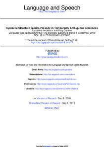
Evaluation involved tests of generated samples on Amazon Mechanical Turk. Participants were asked whether a piece of music was composed by a human or by a machine. Twenty original chorales were selected at random and compared with generated samples. Every pair was played 20 times. This experiment was repeated for fully sampled pieces of music and
39
6.4 Conclusions and Further work
for these with sampled melody line and rest found by beam search with constraints imposed. Constraints at this stage involved removing undesirable dissonances; however not all of theme were removed because of the hierarchical nature of imposing constraints. Samples were lasting one minute length and had tempo of 60 beats per minute so participants could listen them carefully. The results of experiment are depicted in the figure below. Samples
Samples+constraints correct: computer not correct: human
20 18
18 16 number of answers
number of answers
16 14 12 10 8 6
14 12 10 8 6
4
4
2
2
0
correct: computer not correct: human
20
0
2
4
6
8
10
12
14
16
18
20
0
20
22
24
sample number
26
28
30
32
34
36
38
40
sample number
Fig. 6.8 Results obtained in recognition experiment. It is visible that imposing constraints lead to an improvement in quality of samples. Overall results are collected in the table below. Correct means that the participant identified the sample generated as automatically generated correctly. Incorrect means that original music was recognized as generated. Table 6.2 Loss obtained during training for all lines. correct samples 258 samples with constraints 222
incorrect 142 178
percentage correct 0.645 0.555
The experiment show that many mistakes were made during recognizing original music. This might be influenced by the fact that participants did not have much knowledge about music and pay attention to simple details more than to complex, overall structure. Introducing constraints provided visible improvements.
6.4
Conclusions and Further work
The model is able to generate various types of samples and all experiments should be reproducible. The quality of samples has improved after constraints were introduced, which was confirmed by human testers. The way of defining constraints is flexible, however, too strict restrictions can lead to a situation in which sequence satisfying constraints does not exist
42
40
Experiments
because of the hierarchical nature of sampling from the model. To improve the results the training data set could be increased, so that more patterns could be learned from data. Applying constraints is a difficult task, as too strict constraints can decrease the quality of predictions. Nevertheless, the aim of the project, which was to build a system that can generate music that appears to be composed by humans, has been achieved. This is not true for all generated samples, but achieving this performance can be considered as satisfying, given the time scope of the project. The problem, which is left, is that some samples might not obey these constraints at some stages, because constraints can be too strict. Further research could investigate the possibility to go back during this sequential procedure of generating lines of music so if a situation in which no output satisfies constraints a step back is performed. Also, these constraints could be carefully tuned to provide better outputs.
References [1] Hochreiter, Sepp, and Jürgen Schmidhuber. "Long short-term memory." Neural computation 9.8 (1997): 1735-1780. [2] Bishop, Christopher M. Neural networks for pattern recognition. Oxford university press, 1995. [3] MacKay, David JC. Information theory, inference and learning algorithms. Cambridge university press, 2003. [4] Kingma, Diederik, and Jimmy Ba. "Adam: A method for stochastic optimization." arXiv preprint arXiv:1412.6980 (2014). [5] Zeiler, Matthew D. "ADADELTA: an adaptive learning rate method." arXiv preprint arXiv:1212.5701 (2012). [6] Hecht-Nielsen, Robert. "Theory of the backpropagation neural network." Neural Networks, 1989. IJCNN., International Joint Conference on. IEEE, 1989. [7] Nakama, Takéhiko. "Theoretical analysis of batch and on-line training for gradient descent learning in neural networks." Neurocomputing 73.1 (2009): 151-159. [8] Giles, Rich Caruana Steve Lawrence Lee. "Overfiting in Neural Nets: Backpropagation, Conjugate Gradient, and Early Stopping." Advances in Neural Information Processing Systems 13: Proceedings of the 2000 Conference. Vol. 13. MIT Press, 2001. [9] Girosi, Federico, Michael Jones, and Tomaso Poggio. "Regularization theory and neural networks architectures." Neural computation 7.2 (1995): 219-269. [10] Srivastava, Nitish, et al. "Dropout: a simple way to prevent neural networks from overfitting." Journal of Machine Learning Research 15.1 (2014): 1929-1958. [11] Ioffe, Sergey, and Christian Szegedy. "Batch normalization: Accelerating deep network training by reducing internal covariate shift." arXiv preprint arXiv:1502.03167 (2015). [12] Mandic, Danilo P., and Jonathon Chambers. Recurrent neural networks for prediction: learning algorithms, architectures and stability. John Wiley and Sons, Inc., 2001. [13] Jaeger, Herbert. Tutorial on training recurrent neural networks, covering BPPT, RTRL, EKF and the" echo state network" approach. GMD-Forschungszentrum Informationstechnik, 2002.
42
References
[14] Pascanu, Razvan, Tomas Mikolov, and Yoshua Bengio. "On the difficulty of training recurrent neural networks." ICML (3) 28 (2013): 1310-1318. [15] Quintana, V. H., and E. J. Davison. "Clipping-off gradient algorithms to compute optimal controls with constrained magnitude." International Journal of Control 20.2 (1974): 243-255. [16] Zaremba, Wojciech. "An empirical exploration of recurrent network architectures." (2015). [17] Stahlberg, Felix, et al. "Syntactically Guided Neural Machine Translation." arXiv preprint arXiv:1605.04569 (2016). [18] Cuthbert, Michael Scott, and Christopher Ariza. "music21: A toolkit for computer-aided musicology and symbolic music data." (2010). [19] Tokui, Seiya, et al. "Chainer: a next-generation open source framework for deep learning." Proceedings of Workshop on Machine Learning Systems (LearningSys) in The Twenty-ninth Annual Conference on Neural Information Processing Systems (NIPS). 2015. [20] Allauzen, Cyril, et al. "OpenFst: A general and efficient weighted finite-state transducer library." International Conference on Implementation and Application of Automata. Springer Berlin Heidelberg, 2007. [21] Worth, Peter, and Susan Stepney. "Growing music: musical interpretations of Lsystems." Workshops on Applications of Evolutionary Computation. Springer Berlin Heidelberg, 2005. [22] Burraston, Dave, and Ernest Edmonds. "Cellular automata in generative electronic music and sonic art: a historical and technical review." Digital Creativity 16.3 (2005): 165-185. [23] webpage http://tones.wolfram.com/, accessed on 20.06.2016 [24] Holtzman, S. R. "Using generative grammars for music composition." Computer Music Journal 5.1 (1981): 51-64. [25] McCormack, Jon. "Grammar based music composition." Complex systems 96 (1996): 321-336. [26] Eck, Douglas, and Juergen Schmidhuber. "A first look at music composition using lstm recurrent neural networks." Istituto Dalle Molle Di Studi Sull Intelligenza Artificiale 103 (2002). [27] Eck, Douglas, and Juergen Schmidhuber. "Finding temporal structure in music: Blues improvisation with LSTM recurrent networks." Neural Networks for Signal Processing, 2002. Proceedings of the 2002 12th IEEE Workshop on. IEEE, 2002. [28] Liu, I., and Bhiksha Ramakrishnan. "Bach in 2014: Music Composition with Recurrent Neural Network." arXiv preprint arXiv:1412.3191 (2014).
References
43
[29] Conklin, Darrell. "Music generation from statistical models." Proceedings of the AISB 2003 Symposium on Artificial Intelligence and Creativity in the Arts and Sciences. 2003. [30] Biles, John. "GenJam: A genetic algorithm for generating jazz solos." Proceedings of the International Computer Music Conference. INTERNATIONAL COMPUTER MUSIC ACCOCIATION, 1994. [31] Johanson, Brad, and Riccardo Poli. GP-music: An interactive genetic programming system for music generation with automated fitness raters. University of Birmingham, Cognitive Science Research Centre, 1998. [32] Srinivas, Mandavilli, and Lalit M. Patnaik. "Genetic algorithms: A survey." Computer 27.6 (1994): 17-26. [33] Boulanger-Lewandowski, Nicolas, Yoshua Bengio, and Pascal Vincent. "Modeling temporal dependencies in high-dimensional sequences: Application to polyphonic music generation and transcription." arXiv preprint arXiv:1206.6392 (2012). [34] Pachet, François, and Pierre Roy. "Markov constraints: steerable generation of Markov sequences." Constraints 16.2 (2011): 148-172. [35] Van Der Merwe, Andries, and Walter Schulze. "Music generation with Markov models." IEEE MultiMedia 3.18 (2011): 78-85. [36] Theis, Lucas, Aäron van den Oord, and Matthias Bethge. "A note on the evaluation of generative models." arXiv preprint arXiv:1511.01844 (2015). [37] Bishop, Christopher M. "Pattern recognition." Machine Learning 128 (2006). [38] Koehn, Philipp. "Pharaoh: a beam search decoder for phrase-based statistical machine translation models." Conference of the Association for Machine Translation in the Americas. Springer Berlin Heidelberg, 2004. [39] article available at http://karpathy.github.io/2015/05/21/rnn-effectiveness/, accessed on 21.07.2016 [40] Mozer, Michael C. "Neural network music composition by prediction: Exploring the benefits of psychoacoustic constraints and multi-scale processing." Connection Science 6.2-3 (1994): 247-280. [41] Hwang, Chii-Ruey. "Simulated annealing: theory and applications." Acta Applicandae Mathematicae 12.1 (1988): 108-111. [42] Chomsky, Noam. Topics in the theory of generative grammar. Vol. 56. Walter de Gruyter, 1966.
Appendix A
A.1
Grammars and Weighted Finite State Automata
The notion of formal grammar was introduced by Chomsky [42] as follows: Definition. Let Σ denote finite alphabet. A grammar G is a four tuple (S, R, T, N), where S ∈ Σ is a start symbol, N set of non-terminals disjoint from Σ, T ⊂ Σ set of terminals and R set of rules of the form (Σ ∪ N)∗ N(Σ ∪ N)∗ → (Σ ∪ N)∗ . If grammar G is defined, strings with symbols from Σ can be defined with derivation: Definition. Given a grammar G and a, b ∈ (Σ ∪ N)∗ it is said that b can be derived from a if and only if: ∃s1 ,s2 ,r1 ,r2 ∈(Σ∪N)∗ a = s1 r1 s2 , r1 → r2 ∈ R, b = s1 r2 s2
(A.1)
Set of all strings in Σ∗ that can be created by applying derivations from start symbol S is called the language defined by a grammar. Arbitrary grammar can be very complex. Context-free grammars have only one nonterminal at the right hand side of rules and hence they define smaller subclass of grammars. Context-free grammars can be transformed into probabilistic context-free grammars by defining a probability distribution over all available derivations. This subfield of grammars can be conveniently described with the help of the notion of automaton. A finite state acceptor (FSA) is defined by a set of states and a set of possible transitions between these states, represented as arcs. Each arc of automaton has associated symbol. Two states are distinct, start state and end state. There can be multiple end states.
46 The string is accepted by automaton if and only if there exists a path from start state to end state such that symbols generated during consecutive transitions create this string. As mentioned earlier context-free grammars have only one non terminal on the right hand side of its rules. There is one-to-one correspondence between right context-free grammars and FSA. Intuitively, the corresponding machine would have states defined by nonterminals of grammar and applying a rule corresponds to transition to a new state defined by a nonterminal. Also it is possible to define weights associated with arcs of FSA; the resulting machine is called weighted finite state automata (WFSA). In the same way there is one to one correspondence between WFSA and context-free probabilistic grammars.
A.2
Details of experiments
Samples that were used for tests are stored in : https://www.dropbox.com/sh/ow6luntg6aebwe2/AAAYacmcrTnkzsz4U-h2xhPSa?dl=0 There are divided to three folders, namely original, in which original chorales are stored, sampled, storying samples which were sampled from model, sampled with constraints, which apply beam search and contains to sampled melody line. Another folder, results, stores screenshots from Amazon Mechanical Turk webpage obtained as results of experiments. Also, zip archive model, contains all scripts that were used for training.