Mar 30, 2005 - Wallflower: Principles and Practice of Background Maintenance. International. Conference on Computer Vision. Corfu, Greece. September ...
IMS 2005 - IEEE International Workshop on Measurement Systems for Homeland Security, Contraband Detection and Personal Safety Orlando, FL, USA, 29-30 March 2005
Background Estimation with Gaussian Distribution for Image Segmentation, a fast approach. Gianluca Bailo1, Massimo Bariani1, Paivi Ijas1, Marco Raggio1 1
Department of Biophysical and Electronic Engineering University of Genova Via Opera Pia 11 A, 16146 Genova, ITALY
their removal, for example. Friedman and Russel [2] have invented a background subtraction method for vehicle detection. In their approach the pixels in the image are classified to three colour distributions corresponding to road, vehicle and shadow colours. These distributions are updated using the EM-algorithm. However this method can only be used for a particular scene for vehicle detection. Stauffer and Grimson [3] used some ideas presented by Friedman and Russel [2] and they model the history of each pixel using Gaussian distributions. These distributions are used to classify the pixels to foreground and background pixels and thus to update the background model. Their method gave some good results with repetitive motions and different lightning conditions. However it suffers from slow learning of the background at the beginning and is not very fast. KaewTraKulPong and Bowden [4] have further improved the method presented by Stauffer and Grimson by using different kinds of update equations and also by adding shadow detection. Also Power and Schonees [5] have presented some new ideas for the updating equations and made some study about different parameters. Some promising results have been gained with these methods, however, each of them still have their drawbacks. Toyama et. al [6] have presented a three-level system for background adaptation. The algorithm works in pixel, region and frame levels in order to solve as many problems as possible. This method can deal well with changing lightning conditions, repetitive motions and new objects brought to background. However the speed of the algorithm can be questioned since it uses information from three different levels.
Abstract – Adaptive background updating is one of the methods used to detect moving objects in video sequences. Many techniques have been presented in this field but there are few mentions about the usage of these methods in real-time applications. We concentrate in the speed of the algorithm and present a method that is fast enough to be used in video surveillance systems. We started from the ideas presented by Gaussian distribution for background generation. Instead of using actively all the pixels in the image we divide the pixels into active and inactive ones. Gaussian distributions are used to model the history of active pixels and to state whether they belong to background or foreground. According to the classification of the previous active pixel also the inactive pixels are classified as a part of the background or foreground. We also reduce the frame frequency and use only every nth frame in the image sequence to construct adaptive background. This article is organised as follows: In Chapter 1 some of the previous work and their results are introduced. In Chapter 2 we first describe the method used by Stauffer and Grimson [3] and then present our new ideas. The results are explained in Chapter 3 and finally a conclusion is given.
Keywords – IEEE Keywords
I. INTRODUCTION AND PREVIOUS WORK Background subtraction is a common method used to detect moving regions in computer vision systems. It simply means the segmentation of the current scene to background (stationary scene) and foreground (the moving objects of interest in the scene). One of the simplest ways to implement background subtraction is to use a constant model for the background. This model is then used to distinguish the moving regions from the background. However, there are many problems with such a method. It can not deal with changes in illumination, objects brought to or removed from the background, shadows, repetitive motion such as the leaves of the trees etc. To solve at least some of these problems more intelligent methods to adapt the background model to the changing environment have been introduced. In order to deal with changing illumination Ridder et al. [1] used Kalman filtering to update the background model. Kalman filters are used to find the most probable background pixels that are then used to update the model. The method does not allow new objects to be added to background nor
0-7803-9120-9/05/$20.00 ©2005 IEEE
II. OUR METHOD Our aim was to find method that could be used in realtime, multiple-camera video surveillance system to distinguish the moving regions in the image. We decided to start from the ideas presented by Stauffer and Grimson [3] as their method seems to be one of the most used ones. Our goal was to be able to improve the speed of this method. The original method of Stauffer and Grimson is presented in detail in chapter 2.1 and in chapter 2.2 we introduce our improvements.
2
A. Modelling pixel histories with Gaussian distributions
to the value of the current pixel the variance of the distribution is set large whereas the weight parameter is given a small value. In order to define which of the K Gaussian distributions describing the history of a pixel result from background and which ones from the foreground the distributions for each pixel are ordered by a factor Z�/V. The distributions that describe the background are expected to have a large weight parameter and small variance. Thus the B first distributions are marked as background distributions. B is defined with the help of the background threshold that is defined by the user and simply means the minimum portion of the data that is considered to result from the background pixels. Thus
Text In their article Stauffer and Grimson [3] use the idea to model the history of each pixel in the image by K Gaussian probability density distributions. The history of a certain pixel {x0, y0} is be defined as a time series {X1, ..., Xt} = {I(x0, y0, i): 1 i t}
(1)
where I refers to the image sequence and Xi is the intensity value of the pixel {x0, y0} at time instant i. For colour images Xi is a vector, for grey level images it is a scalar. The probability to observe a certain pixel value within the history values of the pixel is determined as
b
B = argmin( Zk !�7 )
K
P(Xt) = Zi,t·K(Xt, Pi,t, 6i,t )
k=1
(2)
i=1
If a pixel is matched with one of these B distributions it is marked as a background pixel. Otherwise the pixel is considered as a part of a moving object and thus it is marked as a foreground pixel.
where K refers to the number of Gaussian distributions used. Zi,t is the weight parameter that is used to describe which part of the data is described by the ith Gaussian distribution. K�is a Gaussian distribution that has two parameters: Pt is the mean of the Gaussian distribution at time t and 6t is the covariance matrix at time instant t. Stauffer and Grimson use 3 to 5 distributions to describe the history of each pixel. An on-line K-means approximation is then used to update the parameters of the distributions as new information is gained from new frames. For each frame every new pixel value is compared against the existing Gaussian distributions. A new pixel is said to match a distribution if it is within 2.5 standard deviations from the mean of the distribution. If a pixel matched with one of the weighted Gaussian distributions the mean and the variance of this distribution are updated using the following equations �����Pt = (1 - U)Pt-1 + UXt
(3)
�Vt2 = (1 - U)Vt-12+ U�Xt - Pt)T�Xt - Pt)
(4)
where U = DK�XtŇPk, Vk )
(5)
B. Our approach Instead of using colour images as Stauffer and Grimson did, we decided to convert the images to greyscale and use these images for the background estimation. The usage of grey level images makes the calculation of variance easier and the algorithm becomes somewhat simpler also in other parts. Anyhow this did not make the algorithm fast enough so some further improvements were needed. We left from the assumption that the values of neighbouring pixels have a correlation and thus also the history values of these pixels are correlated. Instead of modelling the history of all the pixels in the image we decided to use the information gained only from every other or every third pixel in the image. Thus the pixels are divided into active and inactive pixels. For example every other pixel in the image is used as active pixel and every other as an inactive pixel. The histories of active pixels are modelled with K Gaussian distributions as described in the previous chapter. Using these distributions it is then stated whether a new active pixel is a part of the background or the foreground. The inactive pixels are classified based again on the correlation assumption. If an active pixel was classified to be a part of the background also the inactive pixel/pixels following the active pixel are stated to belong to the same class. This way it is possible to reduce the number of Gaussian distributions needed to model the background which also reduces the elaboration time significantly. We left from the assumption that the values of neighbouring pixels have a correlation and thus also the history values of these pixels are correlated. Instead of modelling the history of all the pixels in the image we decided to use the information gained only from every other or every third pixel in the image. Thus the pixels are divided
D is the learning rate that is defined by the user and is used to define the learning speed of the background updating. The mean and the variance of an unmatched distribution are not updated. Also the weight parameters of all the distributions belonging to the certain pixel are updated as follows Zk,t = (1 - D)Zk,t-1 + D�0k,t)
(7)
(6)
where 0k,t is 1 for matched distribution and 0 for a distribution that was not matched. If the current pixel did not match with any of the K distributions the distribution with smallest weight associated to that particular pixel is replaced by a new distribution. The mean of this new distribution is set
3
into active and inactive pixels. For example every other pixel in the image is used as active pixel and every other as an inactive pixel. The histories of active pixels are modelled with K Gaussian distributions as described in the previous chapter. Using these distributions it is then stated whether a new active pixel is a part of the background or the foreground. The inactive pixels are classified based again on the correlation assumption. If an active pixel was classified to be a part of the background also the inactive pixel/pixels following the active pixel are stated to belong to the same class. This way it is possible to reduce the number of Gaussian distributions needed to model the background which also reduces the elaboration time significantly.
(a)
(b)
(c)
(d)
(e)
(f)
(g)
III. RESULTS Our system was tested with various video sequences containing repetitive motions, changes in lighting etc. The video sequences used included 25 frames per second. Three Gaussian distributions were used to model the history of each active pixel. All the tests were done using a 1,70GHz Pentium 4 with 256 MB RAM, which has Microsoft Windows 2000 as the operating system. Figure 1 shows the functionality of our system. Figure 1(a) presents the original scene with moving people and cars. Figures 1(b) and 1(c) show the binary motion mask when every pixel in the image is examined as in the original system presented by Stauffer and Grimson [3]. The results of using only every other pixel as an active pixel can be seen in Figures 1(d) and 1(e). Figures 1(f) and 1(g) show the same results when every third pixel is examined. As it can be seen in Figure 1 the binary motion mask barely changes even if the amount of active pixels is decreased. The shapes of the moving objects can be seen in the background a little more clearly when every other or every third pixel is examined. However we are interested in a clear binary motion mask that can be used for motion tracking and can be calculated with a fast algorithm. Neither the changes made to the frame frequency do affect to the visual results. The binary motion mask is clear also when only every other, every fourth or every eighth frame of the sequence is used, for example. Next we studied the elaboration times needed per one frame using a different amount of active pixels and the results are shown in Table 1. As the results demonstrate the reduction in the amount of active pixels also significantly reduces the elaboration times. The variations in elaboration times are due to the different amount of movement in the scene. When using the information of every pixel 14-16 frames per second can be elaborated. Instead of taking only every other pixel as active pixel 24-26 frames per second and 30-32 frames for every third pixel can be elaborated. The effects of our changes to the amount of noise in the binary motion mask were also studied.
Figure 1. Visual results. (a) The original image. Binary motion masks and background estimates when the information was collected from (b)&(c) every pixel, (d)&(e) every other pixel and (f)&(g) every third pixel.
The algorithm always creates some salt and pepper noise to the original binary motion image. This noise is due to the false detections made by the system and thus it is also a good measure for the robustness of the algorithm. The amount of noise created was approximated by calculating the difference image between the original binary motion image and the binary motion image after the usage of morphological operators. Table 1. The times needed to elaborate one frame using our algorithm. Column 1 shows the times using only the algorithm for adaptive backgrounding and column 2 the times when also morphological operations to remove unconnected pixels and unite connected pixels are in use.
4
Only the adaptive background algorithm
Adaptive background + morphological operations
Every pixel active
40-50 ms
50-60 ms
Every other pixel active
20-30 ms
30-40 ms
Every third pixel active
10-20 ms
20-30ms
[4] KaewTraKulPong, P., Bowden, R. 2001. An Improved Adaptive Background Mixture Model for RealtimeTracking with Shadow Detection. In Proc. of 2nd European Workshop on Advanced Video Based Surveillance Systems, AVBS01. Kingston upon Thames. Sept 2001. [5] Power, P.W., Schoonees, J.A. 2002. Understanding Background Mixture Models for Foreground Segmentation. Proceedings Image and Vision Computing. New Zealand. [6] Toyama, K., Krumm, J., Brumitt, B., Meyers, B. 1999. Wallflower: Principles and Practice of Background Maintenance. International Conference on Computer Vision. Corfu, Greece. September 1999.
Table 2. The amount of noisy pixels in the image with different combinations. The percentage of noisy pixels
Every frame used
Every 2nd frame used
Every 4th frame used
Every pixel active
1,60 %
1,61 %
1,63 %
Every other pixel active
1,62 %
1,61 %
1,62 %
Every third pixel active
1,60 %
1,62 %
1,63 %
This difference image shows the false detections made by the system that are the pixels considered to be noise. The number of falsely detected pixels was calculated and compared with the total number of the pixels in the image. Table 2 shows the percentage of noisy pixels when a different number of active pixels and different frame frequencies were used. As it can be seen the amount of active pixels does not affect to the amount of noise created by the system. Neither does the usage of only every nth frame. As the results show we succeeded in our aim to reduce the elaboration time of the algorithm. The improvements made do not affect either to the robustness or the visual results of the system. Some other problems of the algorithm presented by Stauffer and Grimson [3] still remain unsolved. One of the drawbacks is the time needed to learn the background at the beginning and also after sudden changes in lightning. Another problem is that when the moving objects stop they are adapted to the background too fast. These problems will be further studied and remain as future work. IV. CONCLUSIONS We presented an adaptive background method based on the model presented by Stauffer and Grimson [3]. In our method only every other or every third pixel in the image was modelled by Gaussian distributions. The results show that our method is faster than the original system. The ability to detect moving areas and the amount of noise in the binary motion image do not differ from the properties of the original system. Due to the speed and robustness of our method it can be implemented to a real life video surveillance application and can be run with normal computers. We concentrated in the speed of the algorithm so some other problems such as slow learning at the beginning or too fast adaptation of still objects still remain to be solved efficiently in the future. REFERENCES [1] Ridder, C., Munkelt, O., Kirchner, H. 1995. Adaptive Background Estimation and Foreground Detection using Kalman-Filtering. Proceedings of International Conference on recent Advances in Mechatronics, ICRAM'95. June 1995. UNESCO Chair on Mechatronics. Pages 193-199. [2] Friedman, N., Russel, S. 1997. Image segmentation in video sequences: A probabilistic approach. In Proc. of the Thirteenth Conference of Uncertainty in Artificial Intelligence (UAI). August 1-3 1997. [3] Stauffer, C., Grimson, W.E.L. 1999. Adaptive background mixture models for real-time tracking. In IEEE Conference on Computer Vision & Pattern Recognition. Colorado, USA. June 1999. IEEE. Pages 246 – 252.
5