4/4/2018
BAITSSS Overview - Ramesh Dhungel
BAITSSS Overview
Ramesh Dhungel
Research
[email protected] Updated an hour ago
BAITSSS Overview
Share
BAITSSS Variables
BAITSSS Evaluation
BAITSSS Future Applications
Publications
BAITSSS Overview BAITSSS Variables
Contents
BAITSSS Evaluation
1 Background 2 Introduction 3 Approach (see BAITSSS Variables) 4 Data (point or gridded) 5 References
BAITSSS Future Applications
Backward-Averaged Iterative Two-Source Surface temperature and energy balance Solution (BAITSSS) Evapotranspiration Model Background The majority of the operational remote sensing-based surface energy balance models compute evapotranspiration (ET) in a large spatial resolution, which is primarily facilitated by instantaneous thermal-based surface temperature, where thermal images are not readily available in the larger spatial (~ 30-meter) and temporal resolution (~ hourly and daily) concurrently. These models utilize instantaneous evaporative fraction (ETrF) or evaporative fraction (EF) and reference ET (ETr) while computing the seasonal ET, while any error in these fractions and ETr can propagate because of the absence of the cloud-free images along with multiple other factors (i.e. lack of direct physical based surface energy and water balance model to incorporate irrigation and precipitation for both bare soil and vegetative canopy). To address some of these difficulties, Dhungel et al.,2016 developed a weather-based physical ET algorithm by integrating the surface energy balance and soil water balance.
Introduction Backward-Averaged Iterative Two-Source Surface temperature and energy balance Solution (BAITSSS), Dhungel et al., 2016 - developed by Dr. Ramesh Dhungel and Water Resources Group of Kimberly Research and Extension Center, University of Idaho between 2010 and 2014 (continually modified and improved), a physically-based evapotranspiration (ET) model capable of point scale and landscape simulation of soil water using a vegetative canopy, soils and weather data. BAITSSS uses Python Shell based NumPy and Geospatial Data Abstraction Library (GDAL) programming (open-source) in hourly or smaller time steps in 30-meter or smaller grids; and automated gridded weather data from NLDAS (or weather stations) and vegetation indices such as measured leaf area index (LAI) or satellite input acquisition (Normalized Difference Vegetation Index (NDVI) and LAI).
Approach (see BAITSSS Variables) https://sites.google.com/site/dhun9265/BAITSSS
1/6
4/4/2018
BAITSSS Overview - Ramesh Dhungel BAITSSS establishes radiative, convective, and conductive components of the surface energy balance for soil and canopy surfaces. BAITSSS simulates environmental variables in hourly or smaller time (desired time based on available input) steps in a point or 30-meter grids (~ Landsat pixel spatial resolution) (see BAITSSS Evaluation using 15-minute point weather data and hourly gridded weather data). BAITSSS assumes the vertical transfer of fluxes, vapor pressure, and water without lateral interactions between the cells. BAITSSS integrates fluxes from soil and canopy using the fraction of vegetation cover (fc) based on the vegetation indices. BAITSSS utilizes the standard and complete surface energy balance with the fundamental aerodynamic equations of latent heat flux (LE) and sensible heat flux (H) combined with a Jarvis-type canopy resistance (rsc) model (Jarvis, 1976). BAITSSS adopts some primary resistances formulation from Jarvis, 1976; Sun, 1982; Shuttleworth and Wallace, 1985; Choudhury and Monteith, 1988. BAITSSS computes the sensible heat flux of soil (Hs) and canopy (Hc) as a residual in the surface energy balance, which is internally calibrated while computing the soil surface temperature (Ts) and canopy temperature (Tc) (Figures 1 and 2). BAITSSS estimates ground heat flux based on Hs or Rn_s (Allen et al., 2011) assuming no contribution from the vegetated portion.
Figure 1: BAITSSS Latent heat (LE) (left) and Sensible heat flux (H) (right) model (Dhungel et al.,2016). BAITSSS iteratively solves the surface energy balance components with Monin-Obukhov stability parameters for each time step to calculate the surface temperature at the soil surface (Ts) and canopy level (Tc) (Figure 2, (Dhungel et al,, 2016)).
https://sites.google.com/site/dhun9265/BAITSSS
2/6
4/4/2018
BAITSSS Overview - Ramesh Dhungel
Figure 2: Flow chart of BAITSSS convergence (Dhungel et al.,2016). Canopy resistance (rsc) computed from the Jarvis-type formulation uses weighing functions representing plant response to solar radiation (F1), air temperature (F2), vapor pressure deficit (F3), and soil moisture at the root zone (F4) (Alfieri and Niyogi, 2008; Kumar et al., 2011), each varying between 0 (infinite resistance) to 1 (no resistance).
https://sites.google.com/site/dhun9265/BAITSSS
3/6
4/4/2018
BAITSSS Overview - Ramesh Dhungel
Figure 3: a) F4 function for Jarvis-type model developed from available water fraction (AWF) (Anderson et al., 2007, Dhungel et al.,2016), b) An illustration of the relationship between soil surface resistance (rss) and soil surface moisture (θsur) (Sun, 1982). BAITSSS implements a two-layered soil water balance model, i.e., soil surface (100 mm) and root zone (500 mm - 2000 mm) to track soil evaporation (Ess) and transpiration (T) separately (Figure 3).
Figure 4: a) An illustration of BAITSSS utilizing hourly NLDAS and linearly interpolated NDVI and LAI from satellite acquisition (left), b) BAITSSS soil water balance model (right) (Dhungel et al.,2016). BAITSSS restricts the soil surface and root zone moisture to the field capacity, i.e., water above field capacity either become run-off or deep percolated below the root zone. BAITSSS simulates irrigation in agricultural landscape using Management Allowed Depletion (MAD) and threshold soil moisture at the root zone (Figures 4b and 5).
https://sites.google.com/site/dhun9265/BAITSSS
4/6
4/4/2018
BAITSSS Overview - Ramesh Dhungel
Figure 5: BAITSSS irrigation sub-model with different soil moisture and parameters (Dhungel et al.,2016). BAITSSS is intended to be a tradeoff between complexity and accuracy, to achieve operational ease with minimum data requirements and improve Ess and T partitioning.
Data (point or gridded) BAITSSS generates a large number of variables primarily from five major meteorological forcing (see BAITSSS Variables). Meteorological forcing Gridded hourly weather data from NLDAS ~ 12.5 km Incoming solar radiation Wind speed Air temperature Relative humidity or specific humidity for the actual vapor pressure Precipitation Non-meteorological inputs (satellite-based indices from EarthExplorer) Vegetation indices (NDVI, LAI) Elevation (DEM) Soil data (field capacity, wilting point, and saturated soil moisture) Supplementary inputs National Land Cover Database (NLCD) Cropland data layer (CDL)
References Dhungel, R., Allen, R. G., Trezza, R., & Robison, C. W. (2016). Evapotranspiration between satellite overpasses: methodology and case study in agricultural dominant semi‐arid areas. Meteorological Applications, 23(4), 714-730.
https://sites.google.com/site/dhun9265/BAITSSS
5/6
4/4/2018
BAITSSS Overview - Ramesh Dhungel Dhungel, R., Allen, R. G., & Trezza, R. (2016). Improving iterative surface energy balance convergence for remote sensing based flux calculation. Journal of Applied Remote Sensing, 10(2), 026033. Sun, S.F. (1982). Moisture and heat transport in a soil layer forced by atmospheric conditions. M.S. Thesis, Department of Civil Engineering, University of Connecticut. Dhungel, R., Aiken, R., Colaizzi P., Lin, X., O’Brien, D., Baumhardt, L., Brauer, D., Marek, G., Steve Evett (2018). Landscape-scale crop water productivity model supporting multiyear water management decisions. Central Plains Irrigation Association 2018 Conference, Colby, KS, 2018. Dhungel, R., Aiken, R., Colaizzi P., Lin, X., O’Brien, D., Baumhardt, L., Brauer, D., Marek, G., Steve Evett (2018). Landscape-scale crop water productivity model supporting multiyear water management decisions. OAP Workshop March 27-29 2018 Lubbock Texas.
Copyright © 2018, Ramesh Dhungel, Ph.D., Kansas State University.
Report Abuse
https://sites.google.com/site/dhun9265/BAITSSS
|
Remove Access
| Powered By
Google Sites
6/6
4/4/2018
BAITSSS Variables - Ramesh Dhungel
BAITSSS Variables
Ramesh Dhungel
Research
[email protected] Updated 9 hours ago
BAITSSS Overview
Share
BAITSSS Variables
BAITSSS Evaluation
BAITSSS Future Applications
Publications
BAITSSS Overview BAITSSS Variables
BAITSSS Variables
BAITSSS Evaluation
Table 1: BAITSSS variables and imposed limits (Dhungel et al., 2016)
BAITSSS Future Applications Variable
Symbol
Min.
Max.
Units
Actual vapor pressure of the air
ea
-
-
kPa
Aerodynamic resistance between the substrate and canopy height (d + zom)
ras
-
-
m s-1
Aerodynamic resistance from canopy height to blending height
rah
1
500
m s-1
Air Temperature
Ta
-
-
K
Albedo canopy
αc
0.15
0.24
-
Albedo soil
αs
0.15
0.28
-
Atmospheric density
ρa
-
-
Kg m-3
Bulk boundary layer resistance of the vegetative elements in the canopy
rac
0
5000
m s-1
Canopy resistance
rsc
0
5000
m s-1
Canopy temperature
Tc
265
350
K
Combined (bulk) Sensible heat flux
H
-200
500
W m-2
Emissivity for canopy portion
εo_c
-
-
-
Emissivity for soil portion
εo_s
-
-
-
Fraction of vegetation cover
fc
0.05
1
-
Friction velocity
u*
0.01
500
m s-1
Ground heat flux
G
-200
200
W m-2
https://sites.google.com/site/dhun9265/BAITSSS/BAITSSS-Variables
1/3
4/4/2018
BAITSSS Variables - Ramesh Dhungel Height of canopy
hc
-
-
m
Latent heat of vaporization for vegetation portion
λc
-
-
Incoming longwave radiation
RL↓
-
-
W m-2
Incoming solar radiation
RS↓
-
-
W m-2
Integration constant
Z1
-
-
m
Latent heat flux for canopy
LEc
-
-
W m-2
Latent heat flux for soil
LEs
-
-
W m-2
Latent heat of vaporization for soil portion
λs
-
-
J/kg
Leaf area index
LAI
fc
-
-
Management allowable depletion
MAD
-
-
%
Mean boundary layer resistance per unit area of vegetation
rb
0
-
s m-1
Measurement height
Z
-
-
m
Minimum roughness length
zos
0.01
-
m
Net Radiation
Rn
-
-
W m-2
Net Radiation of canopy portion
Rn_c
-
-
W m-2
Net Radiation of soil portion
Rn_s
-
-
W m-2
Readily available water
RAW
-
-
m3 m-3
Relative humidity
RH
-
-
%
Roughness length of heat
zoh
-
-
m
Roughness length of momentum
zom
0.01
-
m
Saturation vapor pressure at the canopy surface
eoc
-
-
kPa
Saturation vapor pressure at the soil surface
eos
-
-
kPa
Sensible heat flux for canopy portion
Hc
-200
500
W m-2
Sensible heat flux for soil portion
Hs
-200
500
W m-2
Soil moisture at field capacity
θfc
-
-
m3 m-3
Soil moisture at root zone
θroot
-
-
m3 m-3
Soil moisture at saturation
θsat
-
-
m3 m-3
Soil moisture at soil surface
θsur
-
-
m3 m-3
J/kg
https://sites.google.com/site/dhun9265/BAITSSS/BAITSSS-Variables
2/3
4/4/2018
BAITSSS Variables - Ramesh Dhungel Soil moisture at wilting point
θwp
-
-
m3 m-3
Soil surface evaporation
Ess
0.0001
-
mm hr-1
Soil surface resistance
rss
35
5000
m s-1
Soil surface temperature
Ts
265
350
K
Specific heat capacity of moist air
cp
Stability correction parameter
ψ
-
-
-
Threshold moisture content
θt
-
-
m3 m-3
Total available water
TAW
-
-
m3 m-3
Transpiration
T
0.0001
-
mm hr-1
Wind speed
uz
-
-
m s-1
J (kg K)-1
Copyright © 2018, Ramesh Dhungel, Ph.D., Kansas State University.
Report Abuse
https://sites.google.com/site/dhun9265/BAITSSS/BAITSSS-Variables
|
Remove Access
| Powered By
Google Sites
3/3
4/4/2018
BAITSSS Evaluation (Ramesh Dhungel)
BAITSSS Evaluation
Ramesh Dhungel
Research
BAITSSS Overview
[email protected] Updated a minute ago
BAITSSS Overview
Share
BAITSSS Variables
BAITSSS Evaluation
BAITSSS Future Applications
Publications
BAITSSS Overview >
BAITSSS Variables BAITSSS Evaluation BAITSSS Future Applications
BAITSSS Evaluation Point Scale ET BAITSSS was executed and evaluated with the 15-minute ground-based weather data ( ~ 13,000 times) and later hourly averaged to compare the lysimeter ET, measured surface temperature from IRT, and net radiation from net radiometers (only a small section of the results is presented here) for a fully irrigated drought-tolerant corn (Zea mays L. cv. PIO 1151) between May 23 (DOY 143) and September 26 (DOY 270), 2016 for continuous 127 days in a highly advective weather of Bushland, TX. The evaluation period includes from planting to maturity with a wide range of environmental (wetting, drying, and environmental cooling process like precipitation), surface (bare, partial, and full cover), and plant physiological conditions (growing to leaf senescence period). The simulated surface temperature from BAITSSS mimicked the behavior of IRT (for both drying and wetting period) with some positive bias during the complete canopy cover in certain hours of the day (11 am - 2 pm, possibly due to the highly advective environment), though simulated ET was statistically similar to lysimeter during this period. BAITSSS was able to predict ET, surface energy balance fluxes, and other variables with a reasonable accuracy while compared to lysimeter, ground-based IRT, and net radiometers. Comparison between BAITSSS and lysimeter ET (Figures 6a and 6b) with a linearly interpolated LAI from destructive sampling method in a semi-arid advective climate of Bushland, Texas between 05/22/2016 and 09/27/2016.
https://sites.google.com/site/dhun9265/BAITSSS/BAITSSS-Evaluation
1/3
4/4/2018
BAITSSS Evaluation (Ramesh Dhungel)
a)
b) Figure 6: a) Comparison (Uncalibrated blind test) of daily evapotranspiration (ET), lysimeter, and revised BAITSSS ET, b) daily and hourly ET scatterplot of fully irrigated corn between May 22 (DOY 143) and September 26 (DOY 270), 2016, Bushland, TX.
Landscape ET Evapotranspiration (ET) from BAITSSS using hourly North American Land Data Assimilation System (NLDAS) (~ 12.5 km resolution meteorological data) and satellite-based Landsat 7 and 8 (30-meter pixel size, Path 31 and Row 36) based on linearly interpolated vegetation indices (NDVI and LAI) in Parmer County, TX (~ 12 miles * 12 miles) between 05/22/2016 and 09/27/2016, by executing BAITSSS each hour ~ 3072 times) (Figure 7).
https://sites.google.com/site/dhun9265/BAITSSS/BAITSSS-Evaluation
2/3
4/4/2018
BAITSSS Evaluation (Ramesh Dhungel)
Figure 7: Preliminary result of the Seasonal landscape ET from BAITSSS masked for the individual crop i.e., corn, at Parmer County, Texas between May 22 (DOY 143) and September 27 (DOY 271), 2016, Bushland, TX.
References Dhungel, R., Aiken, R., Colaizzi P., Lin, X., O’Brien, D., Baumhardt, L., Brauer, D., Marek, G., Steve Evett (2018). Landscape-scale crop water productivity model supporting multiyear water management decisions. Central Plains Irrigation Association 2018 Conference, Colby, KS, 2018. Dhungel, R., Aiken, R., Colaizzi P., Lin, X., O’Brien, D., Baumhardt, L., Brauer, D., Marek, G., Steve Evett (2018). Landscape-scale crop water productivity model supporting multiyear water management decisions. OAP Workshop March 27-29 2018 Lubbock Texas.
Copyright © 2018, Ramesh Dhungel, Ph.D., Kansas State University.
Report Abuse
https://sites.google.com/site/dhun9265/BAITSSS/BAITSSS-Evaluation
|
Remove Access
| Powered By
Google Sites
3/3
4/4/2018
BAITSSS Future Applications - Ramesh Dhungel
BAITSSS Future Applications
Ramesh Dhungel
Research
[email protected] Updated an hour ago
BAITSSS Overview
Share
BAITSSS Variables
BAITSSS Evaluation
BAITSSS Future Applications
Publications
BAITSSS Overview BAITSSS Variables BAITSSS Evaluation BAITSSS Future Applications
BAITSSS Future Applications The success of quantifying various environmental variables including surface and canopy temperature, and ultimately ET would help to develop a multi-year water management plans where agriculture is facing a sharp decline in irrigation withdrawals around the world. Maintaining farm profitability with reduced irrigation can be supported by knowledge and management of risks associated with inter-annual and multi-year water management decisions. A working knowledge of landscape- and regional scale-effects on water dynamics can build on the success of current decision-support tools and identify opportunities to exploit climate-informed water management synergisms at landscape scales. The physicallybased modeling tool like BAITSSS can help to provide critical information: To provide information regarding consumptive water use, net primary productivity, and yield formation for multi-year crop systems ranging from dryland to full irrigation. To develop a tool that supports analysis of water management policies on net economic returns at the farm and regional levels.
References Dhungel, R., Aiken, R., Colaizzi P., Lin, X., O’Brien, D., Baumhardt, L., Brauer, D., Marek, G., Steve Evett (2018). Landscape-scale crop water productivity model supporting multiyear water management decisions. Central Plains Irrigation Association 2018 Conference, Colby, KS, 2018. Dhungel, R., Aiken, R., Colaizzi P., Lin, X., O’Brien, D., Baumhardt, L., Brauer, D., Marek, G., Steve Evett (2018). Landscape-scale crop water productivity model supporting multiyear water management decisions. OAP Workshop March 27-29 2018 Lubbock Texas.
Copyright © 2018, Ramesh Dhungel, Ph.D., Kansas State University.
Report Abuse
https://sites.google.com/site/dhun9265/BAITSSS/Future-Applications
|
Remove Access
| Powered By
Google Sites
1/1