Iterative linear regression by sector: renormalization of cDNA microarray data ..... Tusher VG, Tibshirani R, Chu G: Significance analysis of microarrays applied to.
Iterative linear regression by sector: renormalization of cDNA microarray data and cluster analysis weighted by cross homology. David B. Finkelstein1, Jeremy Gollub1, Rob Ewing1, Fredrik Sterky1, Shauna Somerville1, J. Michael Cherry2 1 2
Department of Plant Biology, Carnegie Institution of Washington, Stanford CA Department of Genetics, Stanford University, Stanford CA
Abstract Two-color DNA microarray data has proven valuable in high-throughput expression profiling. However microarray expression ratios (log2ratios) are subject to measurement error from multiple causes. Transcript abundance is expected to be a linear function of signal intensity (y = x) where the typical gene is nonresponsive. Once linearity is confirmed, applying the model by fitting log-scale data with simple linear regression reduces the standard deviation of the log2ratios. After which fewer genes are selected by filtering methods. Comparing the residuals of regression to leverage measures can identify the best candidate genes. Spatial bias in log2ratio, defined by printing pin and detected by ANOVA, can be another source of measurement error. Independently applying the linear normalization method to the data from each pin can easily eliminate this error. Less easily addressed is the problem of cross-homology which is expected to correlate to cross-hybridization. Pair-wise comparison of genes demonstrate that genes with similar sequences are measured as having similar expression. While this bias cannot be easily eliminated, the effect this probable cross-hybridization can be minimized in clustering by weighting methods introduced here. Introduction to the Iterative Method Empirical observations, validated by statistical tests, indicate that distinct classes of measurement error alter cDNA microarray data. When these measurement errors are detectable and conform to defined models, corrections can be applied during renormalization. However, supporting biological evidence may be required to validate any normalization method. For the Spellman and Sherlock cell cycle data [3], the spatial and signal intensity dependent measurement errors were corrected through renormalization. Re-analysis of the Spellman and Sherlock cell cycle data set begins with a new method of normalization that more accurately reduces the effects of outliers and spatial variation on the arrays. First, all background-corrected signal intensity values are log transformed. Then linear regression is performed where one the signal intensities of channel is predicted by the signals from the other channel. Spatial error is corrected by performing this regression independently for each sector. Slotted printing pins produced these sectors. The microarrays used in the Spellman experiments had four sectors printed with four distinct pins.
1
The result is four linear intensity equations, one for each sector. Next residuals are calculated for each of the four regression lines. Outliers (those residuals where |e| > 2 x std dev of e) are temporarily removed and the four regression functions are recalculated. If the difference in fit between the new and old regression lines is less than .001, as measured by r-squared, then no further residuals are removed. Else, outliers are removed by the same test as above and the iterations continue. Once completely determined, the slope and intercept values are applied as correction factors to the log transformed channel 2 values. The result is that the function of log channel 1 and log channel 2 closely approximates y = x. Then these values are exponentiated, a new ratio is calculated and this ratio is put on the familiar log base2 scale. This renormalization alone has been demonstrated to substantially reduce the standard deviation of log2 ratios. Next, the detection of cross-hybridization was examined. Unlike sector bias, which is directly measurable, cross-hybridization is inferred from expression patterns. The yeast genome is fully sequenced, thus the sequences of PCR fragments were known. Therefore it is possible, with some error, to determine the likely number of transcripts that could cross-hybridize to a given PCR fragment. The correlation between the likelihood of cross-hybridization and the frequency of transcripts with cross-homology is difficult to assess without empirical evidence. It is important to note that modeling the molecular events during hybridization has proven difficult. Therefore, no analysis can be used to correct data. However, a technique can be applied as an informed post hoc method. In this way, such analysis may indicate where biological confirmation experiments are warranted, rather than supply a mathematical solution. Applying Linear Normalization Applying a linear model presumes that the data is or should be linear with respect to intensity. The assumptions that the typical gene is non-responsive and that rare genes are no more likely to respond than abundant genes leads to the adoption of the linear model y = x. This assumption is probably valid for large-scale genome wide arrays, but not for small specialized arrays. Where y is expression under stress condition and x is the expression of genes under the control condition. Only a small class of genes is expected to respond to any given test. So this equation is valid for the typical case and invalid for the biologically responsive genes. We further presume that biologically responsive genes are sufficiently responsive to be distinguished from the typical gene using statistical tests. For these genes of biological interest the residuals of regression should be especially large. For cases where intensity functions are nonlinear (Roger Bumgarner, MGED3 , Stanford, CA)[5] then nonlinear lowess regression methods may be required in stead of the simple linear regression method employed here. In these cases, however, it is still those genes with the highest residuals from the fitted function that are of the greatest interest. In all tested cases, applying a linear model of error combined with the iterative removal of outlying residuals reduces the standard deviation of the final log2ratios. The range of the data is not substantially altered. However, the distribution of the data may change. Frequently, the kurtosis increases, meaning that the tails are more widely dispersed with respect to the standard deviation. and the skew may change in scale and in
2
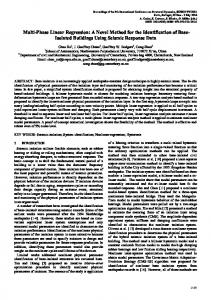
direction. Filtering iteratively normalized data without considering spatial bias, increased the number of genes that are consistently changed at the |log2_ratio|> 2 for 1 of 11 Elutriation arrays by 4.3% (an increase of 9 genes) when compared to data normalized by the SMD default method. When the iterative method is applied each sector to correct spatial problems the number of genes that pass filtering criterion actually decreases. In both cases the overall standard deviation of the data is reduced. Only independent empirical methods can determine whether the differences in analysis methods are removing false positives. Spatial Methods Observation based on a spatial display tool developed for microarrays indicated that spatial problems may exist for several Spellman and Sherlock arrays. Renormalization by sector requires 4 parallel normalizations and assumes that functional groups of genes are not printed together. For many arrays the net result of spatial linear normalization is marginal. However, significant spatial effects have been detected in other cDNA arrays and therefore it is worth testing arrays for the effect. Spatial bias is detectable with a simple ANOVA (y = log2ratio and X = grid #) that yields an F-test and r-squared value. Non-parametric methods such as the KruskalWallis test also serve this function [1]. Our current best estimate is that, if r-squared values are below .05, then spatial error is not significant. Best practice may indicate repeating experiments that are substantially altered, rather than applying sector specific normalization methods, which are post hoc and may only partially repair the effects. Applying the Linear Method by Sector For each of the four independent sectors of each DNA microarray, the iterative simple linear regression technique is applied. As expected many arrays, are not substantially altered by this approach. However, in instances, where outlier sectors are significant, by ANOVA F-tests, differences in normalization are visually evident (Figure 1). Note that the four sectors each have independent patterns with respect to background corrected channel 2 intensity (CH2D). The differences between the SMD method and Iterative method are consistently greater at low intensities: below 150. Each pattern is at a minimum where the linear regression equation for a given sector is equal to the SMD global mean. In this case, there is a clear difference in the minimum of one pattern, which may indicate spatial bias in that sector.
3
Figure 1. The absolute value of the difference between log2_ratio calculated by the SMD method and the Iterative method is plotted on the y-axis. The background-corrected channel 2 intensity is plotted on the x-axis Filtering results Filtering parameters: all spots that have an average intensity of 100 in each channel and a |log2_ratio|>2 in at least 1 array were selected. TABLE I. α-Factor: Elutriation: CDC:
SMD Method 334 179 1204
Iterative Method 269 135 1099
Proportional Change 0.805 0.754 0.913
Note that the Iterative method consistently reduces the number of genes that pass the filters. It also consistently lowers the standard deviation of the log2_ratios in these studies. It does not, however, consistently improve the global correlation between the log2_ratios of any two arrays. Examples of Changed Arrays
4
Column 1:SMD Method
Column 2:Iterative Method
Row A Elut. expt. ID 57
Row B Elut. expt.ID 56
Figure 2. The plots below show the spatial pattern of log2_ratios on two Elutriation arrays (SMD EXPID 56 (row B) and 57(row A) normalized by the SMD method on the left and by the Iterative method on the right. All spots with a log2_ratio greater than 1 appear in red. All spots with a ratio below 1 appear in green. Black spots indicate a flagged spot, white spots have a ratio of 1. Note that the iterative method (Column 2) partially corrects the spatial bias seen in the SMD method (Column1)for both expt. 56 and 57.
Selecting Biologically Significant Genes
5
Once normalization is completed, significantly differential genes are identified by their expression ratios. Because the log2ratios are rarely distributed normally, there are often more candidate genes identified than standard deviation methods would predict. When kurtosis is high, the proportion of differential genes at the tails of the distribution will also be high. Determining which ratios are false positives may be critical to reducing cost and effort of confirmation experiments [4]. The analysis of residuals from simple linear regression affords a screen for these outliers. A linear regression function is subject to the influence individual measurements in direct proportion to their distance from the mean. That is, genes at the extremes have greater leverage (influence) on the predicted regression line then those near the mean of x. Measures of leverage will select a distinct group of genes from a line when compared to those found by residuals. Residuals that are distant from the predicted line may have little leverage if they are especially close to the mean. Since most genes are neither especially rare nor abundant, we expect most biological outliers to be near the mean of x (where x is the control state) and therefore have a high residual and a low leverage [2] If we plot leverage versus the square of the residual we can see a much smaller class of genes are significantly (by standard deviation measures) different by residual measures but not by leverage. Genes that are high in leverage and low in residuals are likely false positives, if they have a differential ratio. Genes that are high in both categories are ambiguous, some can be reasonably expected to be authentically differential. Discerning between these genes is beyond the scope of this simple test.
Leverage
.001343
.000084 .009339
4.8e-13 Normalized residual squared
Figure 3. Leverage vs. residual squared plot of microarray data (from lvr2plot procedure in STATA 6.0 Stata Corp, College Station, TX) .
6
Sequence Similarity in Yeast Arrays The degree to which cross-hybridization might influence microarray expression data was also examined. First, a preliminary analysis was performed that related sequence similarity to the degree of correlation between expression profiles. Several assumptions are made. First, it was assumed that the full length ORFs available from SGD (Saccharomyces Genome Database) approximate the targets actually used on the microarray. This assumption is deemed reasonable, as yeast primer pairs were designed to include as much of the ORFs as possible (Gavin Sherlock, pers. comm.). Second, it was assumed that the degree of sequence similarity between a pair of sequences, as measured by an alignment program such as BLASTN, would approximate the degree of cross-hybridization between those sequences. First, 2,690 ORFS were selected from the original 6,178 yeast ORFs. The selected ORFS were those with the fewest missing expression data values (that is ORFs with greater than 8 missing values across the 62 experiments were excluded). For all pairs of the 2,690 ORFs, the correlation coefficient between the expression profiles was calculated and a BLASTN alignment of the sequences created. For all pairs of ORFs with some degree of homology, the correlation coefficients were extracted and are plotted as two histograms in Figure 2. ORF pairs are divided according to their BLASTN e-values. Correlation coefficients for ORF pairs with BLASTN e-value greater than 1 X 10⁻⁴ are shown in white and those with BLASTN e-value less than 1 X 10⁻⁴ are in red. Relatively few ORF pairs showed significant sequence similarity. 1991 ORF pairs had e-values greater than 1 X 10⁻⁴ and 59 pairs had e-values less than 1 X 10⁻⁴. The set of 1991 ORF pairs had a mean pairwise correlation coefficient of 0.036, whereas the set of 59 ORF pairs with lower e-values had a mean pairwise correlation coefficient of 0.419.
7
Figure 4. Pairwise correlation coefficients of the expression pattern across 62 experiments of yeast ORFS. Red comparisons are highly similar pairs. Note the relative rarity of cross homology and the relative high degree of co-expression amongst the highly similar ORFs. Despite the small numbers, it appears that ORF pairs with a higher degree of sequence similarity are also more likely to exhibit a higher degree of correlation between their expression profiles. The e-value indicates, but does not prove cross-hybridization. It is also possible that genes with high sequence similarity may have similar function and therefore may be authentically co-expressed. Cross-hybridization and the degree to which this may confound results from genome-wide microarray experiments should definitely be considered in the design of future microarrays by printing gene specific probes used wherever possible. Calculating the Weights Weights were assigned to only those genes, which passed two criterion. The pairwise expression with another ORF had to exceed 1e-4 and their BLASTN score had to exceed 100. The BLASTN score was the more stringent criterion, resulting in no expression correlation below 1e-21. 782 pairwise comparisons passed this cut off, representing some 678 ORF's. Weights were first calculated for each pairwise comparison. If an ORF was part of more than one pairwise
8
comparison then the weights were multiplied. Weights were calculated as 0.5 + 0.5(minimum exp/exp). In this case the minimum exponent of the data set was -21. If a given pairwise correlation value was 1e-42 then the weight would be 0.5 + 0.5(-21/-42) = 0.75. The maximum weight was 1 and the minimum weight was 0.16. This method is one of many that should give a reasonable approximation of the range of crosshybridization. However, a method based on empirical evidence of cross-hybridization would be preferable.
Figure 5. Histogram of the weights applied to potentially cross-hybridizing genes. Note that most weights were nearly 0.5, and only a small sub-population is weighted less than 0.25.
Determining Best Practice Best practice of microarray data analysis is directly tied to the application of the data. If the arrays are to be used as rapid screening tools, then sophisticated normalization and analysis may not be necessary. If, however, the object of the experiment is to model subtle biological patterns across gradients of time or treatment, much more complex analysis is required. Furthermore, while statistical measures are useful in measuring and correcting some errors, the most accurate means of determining gene transcript behavior will require empirical evidence. When DNA microarrays are designed to assist the statistical analysis, best practice can be achieved. For example, the replicate printing of a core control group of elements in several locations throughout an array would greatly simplify detection of spatial bias. Also, doping controls that consist of a class of non-homologous RNA transcripts could serve as independent verification of normalization methods. Finally, the correlation of expression amongst elements with high degrees of cross-homology does not prove cross-hybridization. In summary, the
9
combination of careful array design, empirical verification and accurate mathematical models of error will result in the best practice of microarray data analysis. Acknowledgements We would like to acknowledge the National Science Foundation (NSF) for providing functional genomics funding (grant number 9872638) and through it’s postdoctoral fellowship program in bioinformatics (David Finkelstein).
References 1. 2. 3.
4. 5.
Kruskal WH, Wallis WA: The use of ranks in one-criterion variance analysis. Journal of the American Statistical Association 47: 583-621 (1952). Neter J, Wasserman W, Kutner MH: Applied Linear Statistical Models. Irwin, Homewood, Ill (1990). Spellman PT, Sherlock G, Zhang MQ, Iyer VR, Anders K, Eisen MB, Brown PO, Botstein D, Futcher B: Comprehensive identification of cell cycle-regulated genes of the yeast Saccharomyces cerevisiae by microarray hybridization. Mol Biol Cell 9: 3273-97. (1998). Tusher VG, Tibshirani R, Chu G: Significance analysis of microarrays applied to the ionizing radiation response. Proc Natl Acad Sci U S A 98: 5116-21. (2001). Yang YH, Dudoit S, Luu P, Speed TP: Normalization for cDNA Microarray Data UC Berkeley Tech Report (2000).
10