Backward Viterbi Beam Search for Utilizing Dynamic Task Complexity ...
Recommend Documents
This total score S(u1, ··· , uI ) is de- fined as the sum of target scores over the unit sequence u1, ··· , uI with the sum of concatenation scores over the same ...
A more general form of LDM, was first applied in speech recognition in [1]. The system is a multivariate state-space lin- ear dynamic model with canonical forms ...
Scotts Valley, CA 95067. Abstmct- The objective of this ..... The case shown in Fig. 4b is not at- tractive, since it has time varying branch inetrics in the hut terfly.
Mar 30, 1998 - found by dynamic programming, giving the pronunciation /m.e*.k / . ...... [8] R.I. Damper and J.F.G. Eastmond, âPronunciation by analogy: Impact ...
Abstract Many application domains require search and retrieval, which is also .... available task in an auction round in parallel, and the auctioneer allocates each ...
Jan 21, 2017 - Mohamad Hamiruce Marhaban. 2. , Mohd Iqbal Saripan. 2. ,. Toshifumi Moriyama. 3. , and Takashi Takenaka. 3. AbstractâA regularization is ...
they are essentially free from environmental electromagnetic noise and are characterized by a high-speed time response. A beam monitor based on transition ...
The time needed to search for a conjunction target becomes slower as a function of ..... related differences in the psychological refractory period effect?' Psychol.
attributes or alternatives in one choice set or the total number of choice sets faced by a .... This can be explained in the following three situations: (1) if both.
o which often require note-taking (cannot hold all the information that is needed to satisfy the final goal in memory), and o where the specificity of the goal tends ...
Dec 8, 2016 - massive MIMO system with a large number of beams N, the brute-force ... the IEEE International Conference on Communications, London, U.K.,.
munications plc in the United Kingdom. 5 http://www.yahoo.com ... security systems, (3) Car alarms & security, (4) Fire alarms, (5) Gas alarms and (6) Intruder ...
Tampa, FL , 33620, USA. And. William F. Murphy, Jr. IS/DS, University of South ..... factor and elegance was Apple's iPad. The reasoning approach that seems ...
refurbished (ZR) new laser triggering schemes are being .... maintaining gas pressure fixed until a visible spark was ... continuous across the electrode gap.
project Broadway [7], it becomes useful to seek further simplification of the above bit metrics formulas. Lower complexity bit metrics were already inves- tigated in ...
Jul 11, 2012 - Complexity Search for Compressed Neural Networks. Faustino ... neural networks. 1. ... network architecture, Ψ, and data structures used to de-.
element according to the absolute nodal coordinate formulation (ANCF), and an ANCF .... q rigidly attached to the nodes p and q, respectively, are ... the length of the initial undeformed beam, we define the six gen- ..... and l the initial length of
silence models, we add a separate copy of the silence model (Sil) to each tree. In addition, we have ..... Technology Workshop, Austin, TX, pp. 156-161, January ...
the filtered lists in the columns to the right of their selec- tion. This is shown ... ets such as Song Titles, Composers, Periods, Instruments, and Arrangements ...
application area, we selected biomedical laboratory automation on the one ... shows that an extraordinary technical idea or solution will not coercively lead to ...
experiments utilizing a high current, high voltage, microsecond electron accelerator. Thomas A. Spencer, Ronald M. Gilgenbach, and Jin J. Choia).
Dec 20, 2007 - purchasing and web-information extraction is challenging because it consists .... with reference to a domain-specific reasoner such as our task ...
operational cost of cloud service providers in terms of energy ... Keywordsâcloud computing; task scheduling; chaotic;. Symbiotic .... f make minimize span. =α. + âα. (3). IV. CHAOTIC SYMBIOTIC ORGANISMS SEARCH FOR TASK .... 206-210. [14] Sivan
Observatierapportage oefening Bonfire. In opdracht van. Het Ministerie van Binnenlandse Zaken & Koninkrijksrelaties. [9] Klein, M. and Dellarocas, C. and A.
Backward Viterbi Beam Search for Utilizing Dynamic Task Complexity ...
Index Terms: backward Viterbi beam search, dynamic task complexity. 1. Introduction ... programming algorithm, the Viterbi algorithm is performed in a time-synchronous fashion ..... http://cmusphinx.sourceforge.net/html/cmusphinx.php. 2093.
Backward Viterbi Beam Search for Utilizing Dynamic Task Complexity Information Min Tang, Philippe Di Cristo VoiceBox Technologies, Bellevue, Washington, USA [email protected], [email protected]
Abstract The backward Viterbi beam search has not received enough attentions other than being used in the second pass. The reason is that the speech recognition society has long ignored the concept of dynamic complexities of a speech recognition task which can help us to determine whether we should operate Viterbi decoding in forward or backward direction. We use the U.S. street address entry task as one example to show why the analysis of the dynamic task complexity information is important. We then describe the procedure to implement a backward Viterbi decoding system from an existing traditional ASR engine. We evaluated the backward Viterbi search using CMU’s PocketSphinx. The experimental results of the backward Viterbi Search show significant performance improvement over the forward Viterbi decoding system on the U.S. street address entry task. Index Terms: backward Viterbi beam search, dynamic task complexity
W2
...... W1
Figure 1: the Forward Viterbi Algorithm example of two mono-phone words recognition In [3], people proposed to do a two-pass search in order to further speed up the system: the first pass is a forward search which uses a simplified algorithm; the second pass is a backward Viterbi search, which uses information computed in the forward pass to perform a more complicated search in reverse with much less computation load. This approach has shown great speed-up with little performance degradation.
1. Introduction Ever since the Hidden Markov Model (HMM) dominated the Automatic Speech Recognition (ASR) area as the most powerful statistical method for modeling speech signals in the recent two decades[1], the Viterbi algorithm has become the most widely used search algorithm to decode a HMM network in most state-of-the-art ASR systems. As a dynamic programming algorithm, the Viterbi algorithm is performed in a time-synchronous fashion from left to right.
However, the backward Viterbi beam search has not been used in a speech recognition system as the main and standalone decoding approach. We believe the reason is that the dynamic task complexity information is missing in our comprehensive understanding of speech recognition systems, especially in the embedded speech recognition world.
Time-synchronous Viterbi search can be viewed as a breathfirst search with dynamic programming as illustrated in Figure1. Instead of expanding the search paths along a tree, it merges multiple paths that leads to the same search state and keeps only the best path. The standard Viterbi search guarantees to find the global optimal path because it searches through the whole search space. However, in real applications, the search space is very big (the search space of Viterbi algorithm is O(NT), the complexity for the Viterbi algorithm is O(N2T), where N is the number of total HMM states and T is the speech duration[2]). Thus it is impractical to search the overwhelming number of possible paths especially when we have limited resources in embedded devices.
In this paper, we propose an innovative approach to speed up Viterbi beam search, which is to use the forward or backward Viterbi beam search as required by the task based on the analysis of dynamic task complexity. Our experiments have demonstrated that in the U.S. street address entry task, which by its nature favors the backward Viterbi beam search because the complexity of task narrows down along the time line smoothly, we are getting great improvement in both accuracy and speed by using the backward Viterbi beam search. Compared to the conventional forward Viterbi decoding system, our new system was able to run 3 times faster with more than 90% errors reduction on that task.
In order to reduce the computation load, people uses some heuristics to narrow down the search space. A simple way to prune the search space for breath-first search is using beams. Basically instead of keeping all paths at each time, the beam search only looks at a subset of paths whose scores are within a beam to the local-best path so as to achieve a balance between speed and accuracy.
The rest of this paper is organized as follows. Section 2 introduces the concept of dynamic task complexity. Section 3 describes the concept of the backward Viterbi decoding. Section 4 discusses the procedure to build a system that is able to do the backward Viterbi decoding. Experimental results are presented in Section 5.
2090
September 22- 26, Brisbane Australia
2. Dynamic Task Complexity
Dynamic Task Complexity
The problem to evaluate the complexity of a speech recognition task is not trivial, because it not only involves the computation of H(W), which is the language model entropy, but also involves the vocabulary acoustic similarity, speaker variability and the channel characteristics[4]. Theoretically the task complexity should be the estimate of average conditional entropy H(W|O), where W is what the speaker has spoken and O is what the ASR system is hearing. However the direct comparison of estimated H(W|O) could be affected by bad acoustic model estimation, which results in higher conditional entropy with no change in task complexity. Therefore for decades, the speech recognition society has fallen back to use H(W) as the main task complexity measurement.
25
1 1 log 2 800 = 9.7 bit 800
H b ( street | city , state ) = −∑
1 1 log 2 225 = 7.8 bit 225
H b ( street , city , state ) = 5.6 + 9.7 + 7.8 = 23.1 bit
Backward Viterbi Search
Entropy (bit)
Figure 2: Dynamic Task Complexities of the Forward Viterbi search Vs. the Backward Viterbi search on the U.S. Street address entry task As seen from Figure 2, although the whole task complexity is the same no matter whether we proceed the Viterbi decoding in forward direction or backward direction, their inner dynamic task complexities are completely different. When we employ the backward Viterbi search, at each one of the three stages – State recognition, City recognition and Street recognition, the maximum required entropy is 9.7 bits. Compared with the forward Viterbi search, which requires 23.1 bits entropy at the Street recognition stage, the backward Viterbi search requires much smaller beam so as to be able to keep a better balance between speed and accuracy.
3. Backward Viterbi Decoding The Viterbi beam search is basically a network search. So it doesn’t matter whether we are searching from the beginning or from the end of the network. Theoretically when we perform the Viterbi decoding in a backward direction as shown in Figure 3, we should get the same result as what we do in Figure 1 if we set the beam width to be infinite.
W2
......
The dynamic task complexities when we employ the Viterbi search in reverse direction from state to street are: 1 1 (5) H b ( state ) = −∑ log = 5.6 bit 2 50 50 H b (city | state ) = −∑
Forward Viterbi Search
Time
The dynamic task complexities when we employ the Viterbi search in normal direction from street to state are: 1 1 H f ( street ) = − ∑ = 23.1 bit log 2 50 × 800 × 225 50 × 800 × 225 (1) (2) H f (city | street ) = 0 bit
(4)
10
0
Without loss of generality, let’s assume we have 50 states, each state has 800 unique cities (by unique we mean no 2 states can have cities with the same name) and each city has 225 unique streets (cities shares no street names). And to make our life easy, let’s assume all cities and streets are in uniform distribution.
H f ( street , city , state ) = 23.1 + 0 + 0 = 23.1 bit
City,State
State
We use the U.S. street address entry task as one example, where the speaker says the whole street address from street name, city name to state name in one utterance. Naturally we could divide this task into 3 sub-tasks – street recognition, city recognition and state recognition. Depending on how you proceed the Viterbi decoding, the sub-task complexity flow could be very different.
(3)
Street,City,State
15
5
In this paper, we will adopt the same metric to evaluate the task complexity. Different with traditional task complexity estimation approach, we are not only looking at the task as one whole and static block, but also seeing it as the combination of several consecutive sub-tasks and focusing on how the task complexities of sub-tasks change as the search proceeds, which we called – dynamic task complexity.
H f ( state | street , city ) = 0 bit
(Street,City)
Street 20
W1
Figure 3: The Backward Viterbi Algorithm example of two mono-phone words recognition.
(6)
However in a real system, the beam width is never infinite. The same beam could have different influence on the pruning process of the forward search and the backward search because of different dynamic task complexities.
(7)
(8)
2091
v11 v 12 ... v1n
4. Build Backward Viterbi Decoding ASR It is fairly easy to build a Backward Viterbi Decoding system by making some minor changes to an existing forward Viterbi decoding system.
4.1. On Top of Traditional ASR Engines
t12 t23 S1
Right Context R
S2
Reversed triphone: Left Context R
t11
t00 t01
t12
t23 S1
Basically we need to reverse the training text and then re-train the language model. As long as we are using the same training configuration, the reversed LM should generate the same perplexity value on the test set (reversed).
Right Context L
S0
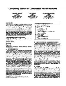
Figure 4: Triphones that should map to the same senone in the original and reverse acoustic models.
4.1.5. Reverse Dictionary Dictionary is reversed by simply reversing the order of all phonemes. For example,
The state transition matrix could be reversed by modifying the matrix so that it generates the same acoustic score without reestimating the state transition probabilities.
“Washington” pronunciation: Pron 1: W AA SH IH NG T AH N Pron 2: W AO SH IH NG T AH N
As show in Figure 4, using the original state transition matrix, the acoustic score of one path is equal to: S = n0t 00 + t 01 + n1t11 + t12 + n2 t 22 + t 23 ,
“Washington” reversed pronunciations: Pron 1: N AH T NG IH SH AA W Pron 2: N AH T NG IH SH AO W
where n0, n1 and n2 correspond to the number of times that the path stays at state S0, S1, and S2. After reversion, the acoustic score is kept the same: S ' = n2t 22 + t12 + n1t11 + t01 + n0t 00 + t 23 = S , where n0,
4.2. On Top of Finite-State-Transducer based ASR Engines
n1 and n2 correspond to the number of times that the path stays at state S0, S1, and S2.
For this kind of ASR engine, since all the grammar, dictionary, acoustic model indices have already been compiled into one network, we could do the trick by simply reversing the network without making any modifications to the acoustic model, grammar and dictionary.
4.1.2. Reverse Feature Vector Simply reversing the audio cannot generate the same feature vectors (the static Cepstral coefficients will be the same, but delta-coefficients are opposite to each other). We need to reverse the feature vectors directly as shown in Figure 5.
Feature Exaction
Frame T
4.1.4. Reverse Language Model
t22
S2
Speech
Frame T-1
Grammar is reversed by simply reversing the order of all rules and terminals. For example, the reverse of $Root = $Intro This Word $Exit; will be: $Root = $Exit Word This $Intro;
5. Experiments We evaluate the backward Viterbi decoding technique in 2 recognition domains using PocketSphinx[5][6] -- CMU's open-source real-time continuous speech recognition system for hand-held devices. In order to make a fair comparison between the forward Viterbi decoding system and the backward Viterbi decoding system, we used the acoustic models that came with the PocketSphinx package as is and didn't make any changes to the Gaussian Mixture Model, the search procedure and the parameter settings. All we did is just reversing the acoustic model, the feature vector, the grammar or language model and the dictionary as described in section 4.1. Since we don't need to re-train or adapt the acoustic model, it requires little effort to make the conventional ASR engine to be able to do the backward Viterbi decoding.
Reversed Feature Vector
Figure 5: Feature vectors must be reversed after the feature extraction module Therefore reversing feature vectors is done by reversing the feature vector array indices as shown in Figure 6.
2092
As seen from Table 2, the system that uses the backward Viterbi decoding technique is not only far more accurate than the forward Viterbi decoding system; it is also 3 times faster.
5.1. TI-Digits Recognition Task The TI-Digits acoustic model that came with the PocketSphinx package contains 670 state-clustered senones. The test set is the standard TI-Digits adult test set which contains 8700 sentences. We have tried both the Finite State Grammar and the statistical language model. The Finite State Grammar is simply a digit loop with the maximum digits length set to 7. The statistical language model is simply a unigram with uniform distribution.
5.2.2. City Recognition After getting the state information, we used the following simple grammar to recognize cities: $Root ::= $garbage* $Cities_in_RecoState RecoState In order to make fair comparison, both systems are using the same configuration settings.
Table 1. Comparison between the forward Viterbi decoding and the backward Viterbi decoding on TI-Digits System Grammar Backward Grammar LM Backward LM
Real-Time Factor 0.02xRT 0.02xRT 0.03xRT 0.03xRT
Table 3. Comparison between the conventional Viterbi and the backward Viterbi on NSCS task: city recognition
Word Error Rate1 0.78% 0.80% 0.71% 0.63%
System Forward Viterbi Backward Viterbi
6. Conclusions In this paper, we have proposed an innovative approach to speed up Viterbi beam search, which is, based on the analysis of dynamic task complexity, using the forward or backward Viterbi beam search as required by the task. Our experimental results have shown that in the situation where the dynamic complexity of the task narrows down along the time line smoothly, we can get great improvements in both the accuracy (more than 90% errors reduction) and speed (3 times faster) by doing the backward Viterbi beam search. It is easy to modify a traditional ASR engine to perform Viterbi search in the reverse direction. And the improvement on accuracy and speed makes this technique suitable for ASR systems running on embedded devices.
5.2. NSCS Address Entry Task: State and City Recognition NSCS stands for address Number, Street name, City name and State name. In a navigation system, it is also referred as One Step Address Entry task because the user gives the whole address in one utterance. NSCS is a very challenging task for the embedded world and it is impractical to conquer this task in one pass because of the huge vocabulary (there are more than 9 million U.S. street-city-state entries and the vocabulary size is about 400,000). So here we adopt a multi-pass strategy – state recognition first, then city recognition followed by house number and street name recognition. The acoustic model that we used is the WSJ0 acoustic model that came with the PocketSphinx package. It contains 4210 state-clustered senones. The test set is collected in VoiceBox and consists of 396 sentences from 6 native American speakers.
7. References [1]
[2]
5.2.1. State Recognition [3]
We used the following simple grammar to recognize states: $Root ::= $garbage* $States It works like a keyword spotting grammar. In order to make fair comparison, we used the same configuration settings for both systems.
[4] [5]
Table 2. Comparison between the conventional Viterbi and the backward Viterbi on NSCS task: state recognition
Forward Viterbi Backward Viterbi
1
Real-Time Factor 0.09xRT 0.03xRT
City Error Rate 82.50% 9.60%
Once again, as seen from Table 3, the backward Viterbi system is 3 times faster than the conventional system with 90% errors reduction.
Table 1 shows the speed and accuracy of the conventional Viterbi decoding system and the backward Viterbi decoding system on TI-Digits task. We can see from this table that the difference between the conventional Viterbi decoding and the backward Viterbi decoding is almost ignorable. Obviously this is what we expected because the TI-Digits task is symmetric thus the Viterbi direction makes no difference.
System
Real-Time Factor 0.164xRT 0.053xRT
[6]
State Error Rate 43.94% 0.51%
All accuracy numbers are evaluated based on top-1 best hypothesis.
2093
Lawrence Rabiner, Biing-Hwang Juang, “Fundamentals of Speech Recognition”, Prentice Hall PTR, Upper Saddle River, NJ, 1993 Xuedong Huang , Alex Acero, Hsiao-Wuen Hon , Raj Reddy, Chapter 12 of “Spoken Language Processing: A Guide to Theory, Algorithm, and System Development”, Prentice Hall PTR, Upper Saddle River, NJ, 2001, pp. 624 Steve Austin, Richard Schwartz and Paul Placeway, “The forward-backward search algorithm”, Proc. of ICASSP, Vol. 1, pp. 697-700, 1991 Frederick Jelinek, “Statistical Methods for Speech Recognition”, The MIT Press, Cambridge, MA, 1998 David Huggins-Daines, Mohit Kumar, Arthur Chan, Alan W Black, Mosur Ravishankar and Alex I. Rudnicky, “PocketSphinx: A Free, Real-Time Continuous Speech Recognition System for Hand-Held Devices”, Proc. of ICASSP, Vol 1, pp. 185-188, 2006. CMU Sphinx Open Source Speech Recognition Engines, http://cmusphinx.sourceforge.net/html/cmusphinx.php