Neural Comput & Applic DOI 10.1007/s00521-014-1716-8
ORIGINAL ARTICLE
Balanced simplicity–accuracy neural network model families for system identification Hector M. Romero Ugalde • Jean-Claude Carmona Juan Reyes-Reyes • Victor M. Alvarado • Christophe Corbier
•
Received: 5 May 2014 / Accepted: 11 September 2014 ! The Natural Computing Applications Forum 2014
Abstract Nonlinear system identification tends to provide highly accurate models these last decades; however, the user remains interested in finding a good balance between high-accuracy models and moderate complexity. In this paper, four balanced accuracy–complexity identification model families are proposed. These models are derived, by selecting different combinations of activation functions in a dedicated neural network design presented in our previous work (Romero-Ugalde et al. in Neurocomputing 101:170–180. doi:10.1016/j.neucom.2012.08.013, 2013). The neural network, based on a recurrent three-layer architecture, helps to reduce the number of parameters of the model after the training phase without any loss of estimation accuracy. Even if this reduction is achieved by a convenient choice of the activation functions and the initial conditions of the synaptic weights, it nevertheless leads to a wide range of models among the most encountered in the literature. To validate the proposed approach, three different systems are identified: The first one corresponds to the unavoidable Wiener–Hammerstein system proposed in
H. M. Romero Ugalde (&) Laboratoire Traitement du Signal et de l’Image, LTSI, Universite´ de Rennes 1, INSERM U1099, 35042 Rennes, France e-mail:
[email protected] J.-C. Carmona Laboratoire des Sciences de l’Information et des Systemes, UMR CNRS 7296, ENSAM, 13100 Aix en Provence, France J. Reyes-Reyes ! V. M. Alvarado Centro Nacional de Investigacion y Desarrollo Tecnologico, CENIDET, 62490 Cuernavaca, Morelos, Mexico C. Corbier LASPI, F-42334 IUT de Roanne, Universite´ de Saint Etienne, Jean Monnet, 42334 Roanne, France
SYSID2009 as a benchmark; the second system is a flexible robot arm; and the third system corresponds to an acoustic duct. Keywords Nonlinear system identification ! Black box ! Neural networks ! Model reduction ! Estimation quality List of symbols Input regressor vector Ju 2 R1"nb Output regressor vector Jy^ 2 R1"na 1"1 Number of pass outputs of the system na 2 R Number of pass inputs of the system nb 2 R1"1 Synaptic weight X 2 R1"1 1"1 Synaptic weight Zb 2 R Synaptic weight Za 2 R1"1 Synaptic weight Vbi 2 R1"1 1"1 Synaptic weight Va i 2 R 1"1 Synaptic weight Zh 2 R Wbi 2 R1"nb Synaptic weight Wai 2 R1"na Synaptic weight WB 2 R1"nb Synaptic weight WA 2 R1"na Synaptic weight Synaptic weight VB 2 R1"1 1"1 Synaptic weight VA 2 R Synaptic weight ZH 2 R1"1 # 1"1 Synaptic weight after training X 2R # 1"1 Synaptic weight after training Zb 2 R Synaptic weight after training Za# 2 R1"1 # 1"1 Synaptic weight after training Vb i 2 R # 1"1 Synaptic weight after training Va i 2 R # 1"1 Synaptic weight after training Zh 2 R Wb#i 2 R1"nb Synaptic weight after training Wa#i 2 R1"na Synaptic weight after training
123
Neural Comput & Applic
WB# 2 R1"nb WA# 2 R1"na VB# 2 R1"1 VA# 2 R1"1 ZH# 2 R1"1 u1 u2 u3 nn 2 R1"1 esim lt st eRMSt u y^
Synaptic weight after training Synaptic weight after training Synaptic weight after training Synaptic weight after training Synaptic weight after training Activation function (linear or nonlinear) Activation function (linear or nonlinear) Activation function (linear or nonlinear) Number of neurons Simulation error Mean value of the simulation error Standard deviation of the error Root mean square (RMS) of the error Input of the neural network Output of the neural network
1 Introduction A model is a mathematical representation of a real system which can be constructed in two ways or in a combination of them [21]. One way is known as physical modeling. The models achieved by this method are adequate approximations of the real process [26]; however, in many cases involving complex nonlinear systems, it is very difficult or impossible to derive dynamic models based on this approach [9, 43]. On the contrary, black-box system identification techniques use general mathematical approximation functions to describe the system’s input/ output relation. One of the most important advantages of these approaches is the limited physical insights required to develop the model [44]; however, as a trade-off, these techniques imply the use of generalized model structures that are as flexible as possible. Often, this generality leads to a high number of parameters [33]. In many engineering fields (automatic control, fault detection, prediction, etc., [1, 9, 19]), accurate process representations with a reduced number of parameters are preferred [9]. For the above reasons, the aim of this paper is to provide a variety of black-box models among the most encountered ones in the literature. These models are derived from a neural network adapted to system identification purposes. In fact, recent research results show that neural networks are very effective for modeling complex nonlinear systems when we consider the plant as a black box [14, 18], especially those that are hard to describe mathematically [23, 40, 45]. However, the main problem of neural networks is that they require a large number of neurons to deal with complex systems [41]. Numerous neurons favor a better approximation but lead to a more complex model [12, 23, 31].
123
Interesting works have been achieved in order to solve the problem of large number of neurons and approximation accuracy. Let us present some works that tend to find the best trade-off between model complexity and approximation accuracy by finding the ‘‘optimal’’ number of neurons. Trial and error is one of these techniques [4]. Different works based on this approach [11, 11, 32, 38, 44, 48, 49, 51] propose models with a good ‘‘quality level,’’ although this procedure is laborious and may not lead to the ‘‘best compromise’’ between model complexity and approximation accuracy [27, 44]. In the sequel, we shall denote for greatest convenience, ‘‘quality’’ as the balance between accuracy and model complexity. Pruning-based techniques have been successfully used for structural optimization [3, 4, 20, 22, 24, 25, 28, 30, 35, 50, 53]. In this approach [5, 13], besides optimizing the number of neurons, the connections between the neurons are also optimized. More recently, other evolutionary techniques have been employed in order to derive ‘‘optimal’’ structures, for example, genetic algorithms (GAs) in [27, 32, 41, 45], dissimilation particle swarm optimization (PSO) in [16], genetic programming (GP) in [9] and a combination of GA and singular value architectural recombination (SVAR) in [17]. As the pruning approach, the previously outlined techniques based on the evolution of the neural network have been successfully applied for structural optimization; however, their main disadvantage is the excessive requirement of time to find the most convenient number of neurons, since the neural network is trained each time the model is modified or restructured [40]. Moreover, to solve the problem of finding the best trade-off between model complexity and model accuracy, a rather subjective criterion is always used to decide whether the evolution of the neural network is appropriate and sufficient. Other techniques are based on the design of the neural network. In [15], a novel time-delay recurrent neural network (TDRNN) is proposed to generate a simple structure. In [7], a neural network using a competitive scheme is proposed in order to provide an effective method with less network complexity. In [29], the selection of an appropriate functional link artificial neural network (FLANN) structure as the backbone of the model offers low complexity by means of a single-layer ANN structure. In [54], a pipeline bilinear recurrent neural network (PBLRNN) is proposed in order to reduce both the model and computational complexities of a bilinear recurrent neural network (BLRNN). In a previous work [36], we proposed a neural network design and a model reduction approach in order to generate balanced accuracy–complexity models. The reduction approach is developed in two steps: The first step consists in training a three-layer neural network under two design conditions. In a second step, the three-layer architecture is
Neural Comput & Applic
transformed into a two-layer representation with a significant reduced number of parameters retaining the approximation accuracy of the previous three-layer model. In this paper, we derive four balanced accuracy–complexity identification models by following this original approach. These provided model types are currently used for control applications [2, 14, 37, 46]. The learning algorithm used to optimize the synaptic weights is the classical steepest descent algorithm with a back propagation configuration. In the sequel, the paper is organized as follows: First, we introduce the neural network structure that allows to derive the balanced accuracy–complexity model families. These models are described in Sect. 3. In Sect. 4, the model reduction approach is applied to one of the proposed model families. In Sect. 5, we discuss the results of the identification of a benchmark system. Subsequently, conclusions and perspectives are given in Sect. 6. The optimization algorithms used to adapt the synaptic weights of the proposed models are given in Appendix 7. In Appendix 8, the reduction approach is applied to the other three model families. Finally, a flexible robot arm and an acoustic duct are identified in Appendices 9 and 10, respectively.
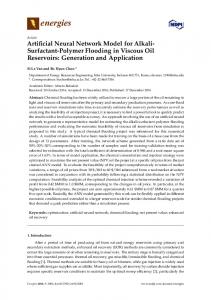
2 Neural network design The neural network design that allows to derive the four balanced accuracy–complexity model families is presented in this section. Figure 1 shows a three-layer neural network with 2 " nn neurons in the input layer, 2 neurons in the hidden layer and 1 neuron in the output layer (2nn-2-1 neural network). The number of neurons in the hidden layer is fixed, and the number of neurons in the input layer (nn neurons used to process the regression input vector and nn neurons used to process the regression output vector) is chosen by the user. As demonstrated in [36], this special configuration allows to reduce the 2nn-2-1 neural network into the 2-1 architecture shown in Fig. 2. The mathematical representation of such neural network architecture is given by (1). y^ðkÞ ¼ Xu3 ðTÞ
T ¼ Zb u2 ðrb Þ þ Za u2 ðra Þ þ Zh nn X rb ¼ Vbi u1 ðJu Wbi Þ ra ¼
i¼1 nn X i¼1
! " Vai u1 Jy^Wai
where: Ju ¼ ½uðk ) 1Þ uðk ) 2Þ . . . uðk ) nb Þ* ! R1"nb Jy^ ¼ ½^ yðk ) 1Þ^ yðk ) 2Þ . . . y^ðk ) na Þ* ! R1"na na is the number of pass outputs of the system
Fig. 1 Recurrent 2nn-2-1 neural network
Fig. 2 Recurrent 2-1 neural network
ð1Þ
nb is the number of pass inputs of the system Wbi ¼ ½Wbi;1 Wbi;2 . . . Wbi;nb *> ! Rnb "1
Wai ¼ ½Wai;1 Wai;2 . . . Wai;na *> ! Rna "1 X; Zb ; Za ; Vbi ; Vai ; Zh !R1 X; Zb ; Za ; Vbi ; Vai ; Zh ; Wbi and Wai are the synaptic weights. u1 ; u2 and u3 are the activation functions (linear or nonlinear) of the neural network.
123
Neural Comput & Applic
where i ¼ 1; 2; . . .; nn and nn is the number of neurons. Now, we shall present the final architecture obtained at the end of the reduction procedure. Figure 2 shows a two-layer neural network with 2 neurons in the input layer (1 neuron used to process the regression input vector and 1 neuron used to process the regression output vector). The mathematical representation of such neural network architecture is given by (2). y^ðkÞ ¼ u3 ðTÞ
T ¼ VB u1 ðJu WB Þ þ VA u1 ðJy^WA Þ þ ZH
ð2Þ
where: VBi ; VAi ; ZH !R1 WB ¼ ½Wb1;1 Wb1;2 . . . Wb1;nb *> ! Rnb "1
WA ¼ ½Wa1;1 Wa1;2 . . . Wa1;na *> ! Rna "1 The aim of this paper is to provide the users with four model families combining the simplicity of the neural network of Fig. 2 [Eq. (2)] and the approximation capabilities of Fig. 1 [Eq. (1)], under some reasonable assumptions as we shall see in the sequel.
y^ðkÞ ¼ XT
T ¼ Zb ðrb Þ þ Za ðra Þ þ Zh nn X rb ¼ Vbi ðJu Wbi Þ ra ¼
i¼1 nn X i¼1
ð5Þ
! " Vai Jy^Wai
Model NARX By selecting u2 ðzÞ ¼ u1 ðzÞ ¼ z and u3 ðzÞ ¼ nonlinear in (1), we obtain: y^ðkÞ ¼ Xu3 ðTÞ T ¼ Zb ðrb Þ þ Za ðra Þ þ Zh nn X rb ¼ Vbi ðJu Wbi Þ ra ¼
i¼1 nn X i¼1
ð6Þ
! " Vai Jy^Wai
The adaptation laws of the synaptic weights, derived according to the discrete time steepest descent gradient, are presented in Appendix 7.
4 Model complexity reduction procedure 3 Identification model families description As already mentioned, four different models can be generated by selecting different combinations of activation functions (u1 ; u2 ; u3 ) in Fig. 1. Let us name these models: Model FF1 By selecting u3 ðzÞ ¼ u2 ðzÞ ¼ z and u1 ðzÞ ¼ nonlinear in (1), we obtain: y^ðkÞ ¼ XT T ¼ Zb rb þ Za ra þ Zh nn X rb ¼ Vbi u1 ðJu Wbi Þ ra ¼
i¼1 nn X i¼1
ð3Þ
! " Vai u1 Jy^Wai
Model FF2 By selecting u3 ðzÞ ¼ u1 ðzÞ ¼ z and u2 ðzÞ ¼ nonlinear in (1), we obtain: y^ðkÞ ¼ XT
T ¼ Zb u2 ðrb Þ þ Za u2 ðra Þ þ Zh nn X rb ¼ Vbi ðJu Wbi Þ ra ¼
i¼1 nn X i¼1
! " Vai Jy^Wai
ð4Þ
Model ARX By selecting u3 ðzÞ ¼ u2 ðzÞ ¼ u1 ðzÞ ¼ z in (1), we obtain:
123
According to the results obtained in [36], this approach provides balanced accuracy–complexity models under the following two conditions. More precisely, the first one is a neural architecture design condition and the second one is a training design condition. Assumption 1 At least one layer should have all its activation functions chosen as linear, that is, u1 ðTÞ ¼ T or u2 ðTÞ ¼ T or u3 ðTÞ ¼ T in Fig. 1. The reader shall notice that Assumption 1 is a classical way to choose the activation functions in the neural network community. Assumption 2 The designer should select the initial condition of the synaptic weights equals group by group, i.e., Vb1 ð0Þ ¼ Vbj ð0Þ; Va1 ð0Þ ¼ Vaj ð0Þ; Wb1 ð0Þ ¼ Wbj ð0Þ and Wa1 ð0Þ ¼ Waj ð0Þ with j ¼ 2; 3; . . .; nn. Even if this is not a classical way to choose the initial conditions of the synaptic weights, full experiments, detailed in [36], demonstrated their validity. Let us remember the theorem presented in [36]: Theorem 1 Consider the neural network whose architecture 2nn-2-1 is expressed in (1) and depicted in Fig. 1, if Assumptions 1 and 2 are fulfilled, then such neural network can be reduced into a 2-1 equivalent architecture (see Fig. 2).
Neural Comput & Applic
Proof Applying the demonstration developed in [36] to the model FF1 given by (3), we have: Step 1. Neural network training under particular assumptions Notice that the model FF1 given by (3) satisfies Assumption 1. According to Assumption 2, let us select the initial conditions of the synaptic weights as follows Vb1 ð0Þ ¼ Vbj ð0Þ; Va1 ð0Þ ¼ Vaj ð0Þ; Wb1 ð0Þ ¼ Wbj ð0Þ and Wa1 ð0Þ ¼ Waj ð0Þ with j ¼ 2; 3; . . .; nn. Once the neural network model given by (3) is trained under these two assumptions, we obtain: y^ðkÞ ¼ X # T
T ¼ Zb# rb þ Za# ra þ Zh# nn # $ X rb ¼ Vb#i u1 Ju Wb#i ra ¼
i¼1 nn X i¼1
ð7Þ
# $ Va#i u1 Jy^Wa#i
As demonstrated in [36], when the initial conditions of the synaptic weights are chosen equals group by group (see Assumption 2), and each group is trained by the same adaptation rule [see (22), (23), (24), (25) in Appendix 7], the final values of the synaptic weights are: Vb#1 ¼ Vb#j ; Va#1 ¼ Va#j ; Wb#1 ¼ Wb#j and Wa#1 ¼ Wa#j with j ¼ 2; 3; . . .; nn. Step 2. Model transformation Let us remember that the synaptic weights are adapted during the neural network training. We can then develop the model transformation. Layer reduction In (7), it is possible to make the following algebraic operations: VB#i VA#i ZH#
#
¼X " #
¼X " #
¼X "
Zb# Za# Zh#
" "
Vb#i Va#i
where VB#1 ¼ VB#j and VA#1 ¼ VA#j (with j ¼ 2; 3; . . .; nn) due to Assumption 2 (Step 1). The three-layer model [Fig. 1, Eq. (1)] is then redefined as a two-layer neural network [Fig. 3, Eq. (8)]. y^ðkÞ ¼ T
T ¼ rb þ ra þ ZH# nn # $ X rb ¼ VB#i u1 Ju Wb#i ra ¼
i¼1 nn X i¼1
ð8Þ
# $ VA#i u1 Jy^Wa#i
Neurons reduction A supplementary transformation is achieved in order to change the 2nn-1 neural network, containing 2 " nn neurons in the input layer (Fig. 3), into a model of two neurons in the input layer (Fig. 2).
Fig. 3 Recurrent 2nn-1 neural network
From Assumption 2 and after ‘‘Layer reduction,’’ we have VB#1 ¼ VB#j ; VA#1 ¼ VA#j ; Wb#1 ¼ Wb#j and Wa#1 ¼ Wa#j (with j ¼ 2; 3; . . .; nn) in (8). The following algebraic operations can be done in (8): nn # $ X VB#i u1 ðJu Wb#i Þ ¼ VB# u1 Ju Wb#1 i¼1
nn X i¼1
# $ VA#i u1 ðJy^Wa#i Þ ¼ VA# u1 Jy^Wa#1
where: VB# ¼ nn " VB#i VA# ¼ nn " VA#i The resulting model after the ‘‘neurons reduction’’ has the mathematical form: # $ # $ ð9Þ y^ðkÞ ¼ VB# u1 Ju Wb#1 þ VA# u1 Jy^Wa#1 þ ZH#
The preceding algebraic manipulations lead to the final simpler model of two neurons (or nn ¼ 1, see Fig. 2) with no necessary further effort to improve the approximation accuracy.
123
Neural Comput & Applic
It is important to note that (9) is in fact entirely equivalent to the complex model (7). Consequently, these two equivalent models have the same accuracy. Thus, it is proved that, by applying Steps 1 and 2, the complex 2nn-2-1 model (Fig. 1) is reduced to a 2-1 model (Fig. 2) with the same accuracy as the complex model. This completes the proof. Remark 1 The fact of choosing the initial conditions of the synaptic weights as proposed in Assumption 2 does not affect the approximation accuracy of the neural network. In this sense, we applied this approach to various applications, such as an acoustic duct, a piezoelectric system, a robot arm and the Wiener–Hammerstein benchmark system, where we always observed the approximation capability preservation in the estimated models. Remark 2 Since the models FF1, FF2, ARX and NARX [see (3), (4), (5) and (6), respectively] satisfy Assumption 1 and can be trained under Assumption 2, we can apply the proposed model reduction approach (see Appendix 8) in order to generate the following ready-to-use models: FF1 after model reduction:
! " y^ðkÞ ¼ VB# u1 ðJu WB# Þ þ VA# u1 Jy^WA# þ ZH#
ð10Þ
y^ðkÞ ¼ VB# u2 ðJu WB# Þ þ VA# u2 ðJy^WA# Þ þ ZH#
ð11Þ
FF2 after model reduction:
ARX after model reduction: y^ðkÞ ¼ Ju WB# þ Jy^WA# þ ZH#
ð12Þ
NARX after model reduction: ! " y^ðkÞ ¼ X # u3 Ju WB# þ Jy^WA# þ ZH#
ð13Þ
These model families have reasonable reduced number of parameters and offer a convenient accurate estimation as shown in the following section. These characteristics are convenient for applying adaptive control [6, 14, 20, 30, 34, 37, 46, 47, 52].
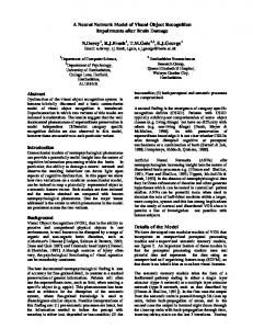
5 Test and results: neuro-identification of the Wiener– Hammerstein case Even if satisfactory results have been driven from experimental setups, we only present in this section results from the identification of the case study reported in the Wiener– Hammerstein benchmark [39]. In order to demonstrate that the proposed model families can be used to represent different systems, a flexible robot arm and an acoustic duct are identified in Appendices 9 and 10, respectively (Figs. 9 and 11).
123
Fig. 4 Wiener–Hammerstein system
Fig. 5 Circuit used to built the static nonlinear system
5.1 The system The DUT is an electronic nonlinear circuit with a Wiener– Hammerstein structure (see Fig. 4). The first filter G1 ðsÞ is designed as a third-order Chebyshev filter (pass-band ripple of 0.5 dB and cutoff frequency of 4.4 kHz). The second filter G2 ðsÞ is designed as a third-order inverse Chebyshev filter (stop-band attenuation of 40 dB starting at 5 kHz). The static nonlinearity is built using a diode circuit (Fig. 5). The system was excited with a band-limited filtered Gaussian excitation signal, and a dataset of 188,000 data was generated, corresponding to 3.6719 s at the sampling frequency of 51,200 Hz (the external excitation starting from sample 5,001 and ending at sample 184,000, approximately). The data are characterized by an extremely low measurement noise level (70 dB below the signal levels). Further details are available in [39]. 5.2 Validation test The dataset available for the benchmark was gathered in two records: the ‘‘estimation data’’ uðtÞ; yðtÞ for t ¼ 1; 2; . . .; 100;000 were manipulated merely for estimating and validating the model; and the ‘‘test data’’ uðtÞ; yðtÞ for t ¼ 100;001; . . .; 188;000 served to evaluate and score the quality of the models, but it was not handled for tuning, as recommended by the automatic control community [39]. We identified the system, using the ‘‘estimation data.’’ Once identified, the model was simulated to estimate the output y^ðtÞ of the system, using no more than the input data at the span of time of the ‘‘test data’’ set (t ¼ 100;001; . . .188;000). The benchmark established the basis to enable the comparison of the models quality. The quality assessment comprises four performance statistical indicators:
Neural Comput & Applic
•
The mean value of the simulation error: lt ¼
•
Model NARX after reduction [see (13)]:
188;000 X
1 esim ðtÞ: 87;000 t¼101;001
ð14Þ
WA# #
The standard deviation of the error (st ): 188;000 X 1 s2t ¼ ðesim ðtÞ ) lt Þ2 87;000 t¼101;001
•
•
ð15Þ
188;000 X 1 ðesim ðtÞÞ2 87000 t¼101;001
ð16Þ
In Eqs. 14–16, the sum is started at t ¼ 101;001 instead of t ¼ 100;001 to eliminate the influence of transient errors at the beginning of the simulation. The root mean square (RMS) value of the error for the estimation data (t 2 ½1;001; 100;000*): e2RMSe ¼
100;000 X 1 ðesim ðtÞÞ2 99;000 t¼1;001
where ð17Þ
5.3 The neural network models The system was identified with the four different models presented above [FF1 (3), FF2 (4), ARX (5) and NARX (6)] with the nonlinear functions classically chosen as tanh [10]. After applying the proposed model reduction method, we obtain the following parameters: Model FF1 after reduction [see (10)]: WB# ¼ ½0:0038 )0:0026
0:0060
)0:0003)0:0095 0:0193*
0:0103
>
¼ ½)0:1130 )0:0623 )0:0057 0:0542*> ¼ 1:6602; VA# ¼ )7:385; and ZH# ¼ )0:0021
Model FF2 after reduction [see (11)]: WB# ¼ ½0:0053 )0:0039 WA# VB#
0:0076
)0:0004)0:0129 0:0252*
¼ ½0:5281 0:2912
0:0138
>
0:0258
)0:2552*>
¼ 1:2818; VA# ¼ 1:6122; and ZH# ¼ )0:002
Model ARX after reduction [see (12)]: WB# ¼ ½0:0200)0:0174 WA# ZH#
)0:0323
0:0183
0:0060
0:0220*
¼ ½0:5968 0:2695
)0:0186
X ¼ 1:5702; andZh# ¼ )8:7947
)0:2388*>
The regressors for the four models are:
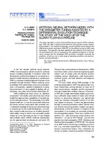
In order to follow the validation tests proposed in [39], we arranged the validation results of the proposed models in Table 1. To complete the exposition of results in the required form, we also present the estimated output in the time domain (Fig. 6), as well as the fast Fourier transform (FFT) of the estimated output signal (Fig. 7). Further information is given through the frequency response function (FRF) of the nonparametric best linear approximation obtained from the test data and the estimated output (see Fig. 8). 5.4 Comments
esim ðtÞ ¼ yðtÞ ) y^ðtÞ
WA# VB#
)0:0210
0:0002
>
Ju ¼ ½uðk ) 1Þ uðk ) 2Þ . . . uðk ) 7Þ* Jy^ ¼ ½y^ðk ) 1Þ y^ðk ) 2Þ . . . y^ðk ) 4Þ*
The root mean square (RMS) of the error: e2RMSt ¼
WB# ¼ ½0:0131 )0:0115
0:0003
0:0282
0:0094
>
0:0343*
¼ ½0:9095 0:4195 ¼ )0:0019
)0:0211
)0:3674*>
The results summary of Table 1 and Fig. 6 expose the relevant performances of three among the four models with respect to the real system behavior, particularly if the number of model parameters is taken into consideration. Here, it seems remarkable that with only 12, 13 and 14 parameters the four proposed models provide a significant level of accuracy. Figures 7 and 8 expose the suitable performances of the provided model families in the frequency domain, particularly in the low frequency that is mainly appreciated by the control community for practical applications. Naturally, we have to compare our approach with respect to another neural network-based system identification technique. The same system was identified by using the nonlinear system identification toolbox in MATLAB 2013. The identification model used was the NLARX model, the nonlinearity estimator is the sigmoid network, and the parameters of the model were estimated by using the Levenberg–Marquardt algorithm. The comparison, realized in terms of the number of parameters np and the validation results proposed in [39], is summarized in Table 2. Moreover, we include in Table 2 results from two other black-box parametric methods presented in SYSID 2009 (Paduart [33] and Mulders [42]). From Table 2, comparing the proposed model families (FF1, FF2, ARX and NARX) with the other black-box system identification approaches (MATLAB, Paduart and Mulders), the validation results (lt ; st ; eRMSt and eRMSe ) of
123
Neural Comput & Applic Table 1 Validation results
st ð"10)3 Þ
eRMSt ð"10)3 Þ
eRMSe ð"10)3 Þ
-2.3
48.5
48.6
48.22
-0.55
56.2
56.2
57.1
12
-3.6
53.8
53.9
53.1
13
-14.1
66.5
67.9
68.7
Ref.
np
FF1
14
FF2
14
ARX NARX
lt ð"10)3 Þ
0.4
Amplitude
Amplitude
0.4
−0.2
−0.8 2.925
W−H system Neuromodel Neuromodel after reduction
2.926
2.927
2.928
2.929
−0.8 2.925
2.93
2.926
2.927
2.928
Time (s)
(a)
(b)
2.929
2.93
2.929
2.93
0.4
Amplitude
Amplitude
W−H system Neuromodel Neuromodel after reduction
Time (s)
0.4
−0.2
W−H system Neuromodel Neuromodel after reduction
−0.8 2.925
−0.2
2.926
2.927
2.928
2.929
2.93
−0.2
−0.8 2.925
W−H system Neuromodel Neuromodel after reduction
2.926
2.927
2.928
Time (s)
Time (s)
(d)
(c) Fig. 6 Measured output versus estimated output. a FF1, b FF2, c ARX, d NARX
the MATLAB, PaduartMulders [33] and Mulders [42] models are better. The number of parameters needed, however, is significantly larger (691, 797 and 833 vs 14, 13 and 12). The users must balance accuracy against complexity, according to their own modeling needs. Furthermore, from a user point of view, it seems to be interesting to provide him with a rather simple that guaranties a satisfactory level of accuracy and a very interesting low complexity order.
6 Conclusion Remember that the foremost subject of this paper are the four balanced accuracy–complexity model families. The
123
quality of the results presented in this paper (see Sect. 5 and Appendices 9 and 10) validates the performance of the four models in terms of the announced motivation. The special structure of the neural network used here leads to accurate models with straightforward efforts. Compared with the neural network evolution techniques, the main advantage of the reduction approach, used to derive the proposed ready-to-use models, is the significant decrease in the training time consumption. In fact, a large enough number of neurons are initially chosen, and then after a single training, the model is simplified. Moreover, as it has been observed, the number of neurons initially chosen to identify a system does not affect the complexity of the reduced model families, due to the fact that (1) the number of parameters of the model ARX depends only on the input
Neural Comput & Applic
−2
−2
10
10
−4
−4
10
Amplitude
Amplitude
10
−6
10
−6
10
−8
−8
10
10 W−H system Neuromodel
−10
10
0
0.05
0.1
W−H system Neuromodel
−10
0.15
0.2
0.25
0.3
0.35
0.4
0.45
0.5
10
0
0.05
0.1
Normalized frequency
0.15
0.2
0.25
0.3
0.35
0.4
0.45
0.5
0.45
0.5
Normalized frequency
(a)
(b)
−2
−2
10
10
−3
10
−4
−4
10
−5
Amplitude
Amplitude
10 10
−6
10
−7
−6
10
10
−8
10
−8
10
−9
W−H system Neuromodel
10
0
0.05
0.1
Neuromodel W−H system
−10
0.15
0.2
0.25
0.3
0.35
0.4
0.45
0.5
10
0
0.05
0.1
0.15
0.2
0.25
0.3
0.35
0.4
Normalized frequency
Normalized frequency
(d)
(c) Fig. 7 Output Fourier transform. a FF1, b FF2, c ARX, d NARX
regression vector size (nb ) added to the output regression vector size (na ) and one parameter, i.e., nb þ na þ 1, (2) the number of parameters of the model NARX is na þ nb þ 2 and (3) the number of parameters of the models FF1 and FF2 is na þ nb þ 3. The reader shall notice that from a user point of view, this last result provides a simple and rather optimal practical rule for choosing the model parameters. Finally, we conclude that the obtained identification models correctly represent the benchmark system. Moreover, these models can be used to represent other types of systems (see Appendices 9 and 10). Owing to the mathematical simplicity and the number of parameters of the estimated models, we can assess that the foremost objective of the paper has been reached. It is interesting to remark that the model reduction approach presented in this paper can be applied to all the neural network models that satisfy Assumptions 1 and 2. In a future work, we will present this generalization applied to other classical architectures. Moreover, we will use robust estimation algorithms, such as the mixed L1 ) L2
estimators, in order to try tackling the high-frequency behavior problem.
Appendix 1: Training The adaptation laws of the synaptic weights, derived according to the steepest descent gradient, are as follows: FF1 adaptation algorithms Xðk þ 1Þ ¼ XðkÞ þ geðkÞT
ð18Þ
Zb ðk þ 1Þ ¼ Zb ðkÞ þ geðkÞXrb
ð19Þ
Za ðk þ 1Þ ¼ Za ðkÞ þ geðkÞXra
ð20Þ
Zh ðk þ 1Þ ¼ Zh ðkÞ þ geðkÞX
ð21Þ
Vbi ðk þ 1Þ ¼ Vbi ðkÞ þ geðkÞXZb tanhðJu Wbi Þ
ð22Þ
Vai ðk þ 1Þ ¼ Vai ðkÞ þ geðkÞXZa tanhðJy^Wai Þ
ð23Þ
123
0
0
−20
−20
−40
−40
Amplitude
Amplitude
Neural Comput & Applic
−60 −80 −100
−60 −80
W−H model Neuromodel 0
0.1
0.2
0.3
0.4
−100
0.5
W−H system Neuromodel 0
0.1
Normalized frequency
0.2
0
0
−20
−20
−40 −60 −80
0.1
0.2
0.5
−40 −60 −80
W−H system Neuromodel 0
0.4
(b)
Amplitude
Amplitude
(a)
−100
0.3
Normalized frequency
0.3
0.4
−100
0.5
W−H system Neuromodel 0
0.1
0.2
0.3
0.4
0.5
Normalized frequency
Normalized frequency
(d)
(c) Fig. 8 Frequency response function (FRF). a FF1, b FF2, c ARX, d NARX
Table 2 A comparative assessment with respect to other parametric methods.
Ref.
np
lt ð"10)3 Þ
st ð"10)3 Þ
eRMSt ð"10)3 Þ
eRMSe ð"10)3 Þ
FF1
14
-2.3
48.5
48.6
48.22
FF2 ARX
14 12
-0.55 -3.6
56.2 53.8
56.2 53.9
57.1 53.1
NARX
13
-14.1
66.5
67.9
68.7
16.7
16.1
16.74
MATLAB
691
0.033
Paduart
797
0.48
0.415
0.36
0.418
Mulders
833
0.00441
3.1
2.62
0.63
Wbi ðk þ 1Þ ¼ Wbi ðkÞ þ geðkÞXZb Vbi sech2 ðJu Wbi ÞJu Wai ðk þ 1Þ ¼ Wai ðkÞ þ geðkÞXZa Vai sech2 ðJy^Wai ÞJy^
ð24Þ ð25Þ
FF2 adaptation algorithms
Zh ðk þ 1Þ ¼ Zh ðkÞ þ geðkÞX
ð29Þ 2
Vbi ðk þ 1Þ ¼ Vbi ðkÞ þ geðkÞXZb sech ðrb ÞJu Wbi
ð30Þ
Vai ðk þ 1Þ ¼ Vai ðkÞ þ geðkÞXZa sech2 ðra ÞJy^Wai
ð31Þ
Xðk þ 1Þ ¼ XðkÞ þ geðkÞT
ð26Þ
Wbi ðk þ 1Þ ¼ Wbi ðkÞ þ geðkÞXZb sech2 ðrb ÞVbi Ju
ð32Þ
Zb ðk þ 1Þ ¼ Zb ðkÞ þ geðkÞX tanhðrb Þ
ð27Þ
Wai ðk þ 1Þ ¼ Wai ðkÞ þ geðkÞXZa sech2 ðra ÞVai Jy^
ð33Þ
Za ðk þ 1Þ ¼ Za ðkÞ þ geðkÞX tanhðra Þ
ð28Þ
ARX adaptation algorithms
123
Neural Comput & Applic
Xðk þ 1Þ ¼ XðkÞ þ geðkÞT
ð34Þ
Zb ðk þ 1Þ ¼ Zb ðkÞ þ geðkÞXrb
ð35Þ
and Va#1 ¼ Va#j with j ¼ 2; 3; . . .; nn. Then, in (50), it is indeed possible to make the following algebraic operations:
Za ðk þ 1Þ ¼ Za ðkÞ þ geðkÞXra
ð36Þ
Zh ðk þ 1Þ ¼ Zh ðkÞ þ geðkÞX
ð37Þ
ZB# ¼ X # " Zb#
Vbi ðk þ 1Þ ¼ Vbi ðkÞ þ geðkÞXZb Ju Wbi
ð38Þ
Vai ðk þ 1Þ ¼ Vai ðkÞ þ geðkÞXZa Jy^Wai
ð39Þ
Wbi ðk þ 1Þ ¼ Wbi ðkÞ þ geðkÞXZb Vbi Ju
ð40Þ
Wai ðk þ 1Þ ¼ Wai ðkÞ þ geðkÞXZa Vai Jy^
ð41Þ
NARX adaptation algorithms
ZA# ¼ X # " Za# ZH# ¼ X # " Zh#
WB#i ¼ Vb#i " Wb#i WA#i ¼ Va#i " Wa#i Then, the 2nn-2-1 neuro-model given by (50) becomes: y^ðkÞ ¼ T
T ¼ ZB# u2 ðrb Þ þ ZA# u2 ðra Þ þ ZH# nn X rb ¼ ðJu WB#i Þ
Xðk þ 1Þ ¼ XðkÞ þ geðkÞ tanhðTÞ
ð42Þ
2
Zb ðk þ 1Þ ¼ Zb ðkÞ þ geðkÞXsech ðTÞrb
ð43Þ
Za ðk þ 1Þ ¼ Za ðkÞ þ geðkÞXsech2 ðTÞra
ð44Þ
ra ¼
Zh ðk þ 1Þ ¼ Zh ðkÞ þ geðkÞXsech2 ðTÞ
ð45Þ
Vbi ðk þ 1Þ ¼ Vbi ðkÞ þ geðkÞXsech2 ðTÞZb Ju Wbi
ð46Þ
Vai ðk þ 1Þ ¼ Vai ðkÞ þ geðkÞXsech2 ðTÞZa Jy^Wai
ð47Þ
Wbi ðk þ 1Þ ¼ Wbi ðkÞ þ geðkÞXsech2 ðTÞZb Vbi Ju
ð48Þ
Wai ðk þ 1Þ ¼ Wai ðkÞ þ geðkÞXsech2 ðTÞZa Vai Jy^
ð49Þ
where WB#1 ¼ WB#j and WA#1 ¼ WA#j (with j ¼ 2; 3; . . .; nn) due to Assumption 2. A supplementary transformation is achieved in order to change the redefined 2nn-1 model (51) into a 2-1 representation by the following algebraic operations: nn X ðJu WB#i Þ ¼ nn " ðJu WB#1 Þ ¼ Ju WB#
with g, commonly referred to as learning rate, adapted according to the ‘‘search then convergence’’ algorithm presented in [8].
i¼1 nn X i¼1
ð51Þ
ðJy^WA#i Þ
i¼1
nn X i¼1
ðJy^WA#i Þ ¼ nn " ðJyn WA#1 Þ ¼ Jyn WA#
The resulting model after the model transformation has the following mathematical form: Appendix 2: Reduction methods applied to models FF2, ARX and NARX
y^ðkÞ ¼ ZB# u2 ðJu WB# Þ þ ZA# u2 ðJy^WA# Þ þ ZH#
ð52Þ
Model ARX Let us follow the proposed system identification procedure: Step 1. Neural network training under particular assumptions Once the neural network model given by (5) is trained under Assumptions 1 and 2, we obtain
Model FF2 Step 1. Neural network training under particular assumptions Once the neural network model given by (4) is trained under Assumptions 1 and 2, we obtain: y^ðkÞ ¼ X # T
T ¼ Zb# u2 ðrb Þ þ Za# u2 ðra Þ nn X rb ¼ Vb#i ðJu Wb#i Þ i¼1 nn X ra ¼ Va#i ðJy^Wa#i Þ i¼1
þ
Zh# ð50Þ
Step 2. Model transformation Since the final values of the synaptic weights are: Wb#1 ¼ Wb#j ; Vb#1 ¼ Vb#j ; Wa#1 ¼ Wa#j
y^ðkÞ ¼ X # T
T ¼ Zb# ðrb Þ þ Za# ðra Þ þ Zh# nn X rb ¼ Vb#i ðJu Wb#i Þ ra ¼
i¼1 nn X i¼1
ð53Þ
Va#i ðJy^Wa#i Þ
Step 2. Model transformation Since the final values of the synaptic weights are: Wb#1 ¼ Wb#j ; Vb#1 ¼ Vb#j ; Wa#1 ¼ Wa#j and Va#1 ¼ Va#j with j ¼ 2; 3; . . .; nn. Then, in (53), it is indeed possible to make the following algebraic operations:
123
Neural Comput & Applic
ZH# ¼ X # " Zh# WB#i WA#i
#
¼X " ¼ X# "
Zb# Za#
" "
Vb#i Va#i
" "
y^ðkÞ ¼ X # u3 ðTÞ
Wb#i Wa#i
Then, the 2nn-2-1 neuro-model given by (53) becomes: y^ðkÞ ¼ T
ra ¼
ZH#
T ¼ rb þ ra þ nn X rb ¼ ðJu WB#i Þ
ð54Þ
i¼1
ra ¼
nn X i¼1
ðJy^WA#i Þ
where WB#1 ¼ WB#j and WA#1 ¼ WA#j (with j ¼ 2; 3; . . .; nn) due to Assumption 2. A supplementary transformation is achieved in order to change the redefined 2nn-1 model (54) into a 2-1 representation by the following algebraic operations: nn X ðJu WB#i Þ ¼ nn " ðJu WB#1 Þ ¼ Ju WB# i¼1 nn X i¼1
ðJy^WA#i Þ ¼ nn " ðJy^WA#1 Þ ¼ Jy^WA#
The resulting model after the model transformation has the following mathematical form: y^ðkÞ ¼ ðJu WB# Þ þ ðJy^WA# Þ þ ZH#
ð55Þ
Model NARX Step 1. Neural network training under particular assumptions Once the neural network model given by (6) is trained under Assumptions 1 and 2, we obtain: y^ðkÞ ¼ X # u3 ðTÞ
T ¼ Zb# ðrb Þ þ Za# ðra Þ þ Zh# nn X rb ¼ Vb#i ðJu Wb#i Þ ra ¼
i¼1 nn X i¼1
ð56Þ
Va#i ðJy^Wa#i Þ
Step 2. Model transformation Since the final values of the synaptic weights are: Wb#1 ¼ Wb#j ; Vb#1 ¼ Vb#j ; Wa#1 ¼ Wa#j and Va#1 ¼ Va#j with j ¼ 2; 3; . . .; nn. Then, in (56), it is indeed possible to make the following algebraic operations: WB#i WA#i
¼ ¼
Zb# Za#
" "
Vb#i Va#i
" "
Wb#i Wa#i
Then, the 2nn-2-1 neuro-model given by (56) becomes:
123
T ¼ rb þ ra þ Zh# nn X rb ¼ ðJu WB#i Þ i¼1 nn X i¼1
ð57Þ
ðJy^WA#i Þ
A supplementary transformation is achieved in order to change the redefined 2nn-1 model (57) into a 2-1 representation by the following algebraic operations: nn X ðJu WB#i Þ ¼ nn " ðJu WB#1 Þ ¼ Ju WB# i¼1
nn X i¼1
ðJy^WA#i Þ ¼ nn " ðJyn WA#1 Þ ¼ Jy^WA#
The resulting model after the model transformation has the following mathematical form: y^ðkÞ ¼ X # u3 ððJu WB# Þ þ ðJy^WA# Þ þ Zh# Þ
ð58Þ
Appendix 2: Neuro-identification of a flexible robot arm In order to show the flexibility of the proposed model families, a second system is identified. The data come from a flexible robot arm (see Fig. 9), and the arm is installed on an electrical motor. The applied persisting exciting input, corresponding to the reaction torque of the structure on the ground, is a periodic sine sweep. The output of the system is the acceleration of the flexible arm. This system identification case is issued from an example through DaISy (database for the identification of systems). http://homes. esat.kuleuven.be/*smc/daisy/daisydata.html. The system is identified with the complex 2nn-2-1 neuro-model NARX (683 parameters before reduction) given by (59) with nn ¼ 40; na ¼ 8 and nb ¼ 7. Notice that this neuro-model is derived from the proposed neural network architecture. y^ðkÞ ¼ X tanhðTÞ
T ¼ Zb ðrb Þ þ Za ðra Þ nn X Vbi ðJu Wbi Þ rb ¼ ra ¼
i¼1 nn X i¼1
! " Vai Jy^Wai
ð59Þ
Once the model (59) is trained under Assumptions 1 and 2, Theorem 1 (reduction approach) is applied in order to generate a reduced model of the form of (60).proposed approach has to be compared ! " y^ðkÞ ¼ X # tanh Ju WB# þ Jy^WA# ð60Þ
Neural Comput & Applic Table 3 A comparative assessment with respect to another parametric method Ref.
lt ð"10)3 Þ
st ð"10)3 Þ
eRMSe ð"10)3 Þ
16
-17.86
79.14
79.14
619
-12.02
35.51
35.52
np
NARX MATLAB
10
Fig. 9 Flexible robot arm
0
WB# ¼ ½0:2883 )0:3820 )0:2135
0:0655
0:1339
0:2335*
WA# ¼ ½)0:7387 )0:0914 0:3221 0:3122 )0:3016 )0:0196 0:3362*
)0:0821
−10
Amplitude
where the 16 parameters characterizing the system are as follows: Proposed NARX model:
−20 −30 −40
)0:0812
X # ¼ )1:4623
Naturally, we have to compare our approach with another black-box system identification method. For example, the same system is identified with the nonlinear system identification toolbox in MATLAB 2013. Here, the identification model used is the NLARX model, and the nonlinearity estimator is the sigmoid network with 5 units, na ¼ 6 and nb ¼ 10. The 619 parameters of the MATLAB model are estimated by using the Levenberg–Marquardt learning algorithm. The comparison, realized in terms of the number of parameters np and the validation results proposed in SYSID 2009 [39], is summarized in Table 3. In order to compare the performances of both models, the frequency response function (FRF) that is mainly appreciated by the users in practical applications is computed from the measured data and the estimated output of both, the proposed neuro-model NARX and the NLARX model obtained by using the toolbox of MATLAB (see Fig. 10). Comments Figure 10 exposes the interest of using neural networks, since the estimated models accurately represent the system behavior in a large frequency range. Confronting the two black-box models (see Table 3), the deviation errors (st and eRMSe ) of the MATLAB model are only two times better, but the number of parameters is substantially larger (619 vs 16). Conversely, in terms of lt , the two models have almost the same accuracy, despite the use of a simple gradient training algorithm in the
Robot Arm Proposed neuro−model NARX
−50 −60
Toolbox of Matlab 0
0.1
0.2
0.3
0.4
0.5
Frequency (Hz)
Fig. 10 Frequency response function (FRF)
computation of the proposed NARX model. Remember that the main objective in this paper is to propose to the user a rather simple and efficient way to find a good balance between accuracy and complexity.
Appendix 3 :Neuro-identification of an acoustic duct In order to show the flexibility of the proposed model families, a third system is identified. This experimental device is an acoustic waves guide made of Plexiglas, used to develop an active noise control (see Fig. 11). One end of the duct is almost anechoic and the other end is opened. The identification input signal is a pseudo-random binary sequence (PRBS) with a length L ¼ 210 ) 1 and level +3 V sufficiently exciting applied to the control loudspeaker. The sampling period is TS = 500 ls. In order to model, the first propagative modes of the waves guide (also called the secondary path) which lye in the frequency range ½0; 1;000 Hz*. We shall use several data set of the same length, namely 1,024, measured by the output microphone. A prior measurement of the propagation delay confirms the analytical value s , 7TS. This system is identified with the complex 2nn-2-1 neuro-model FF1 (1,418 parameters before reduction) given by (61) with nn ¼ 40; na ¼ 15 and nb ¼ 18.
123
Neural Comput & Applic Table 4 A comparative assessment with respect to another parametric method Ref.
lt
st
eRMSe
35
-0.00002
0.9428
0.9428
1,519
-0.02144
0.9067
0.9070
np
FF1 MATLAB
0
10
Amplitude
Fig. 11 Schematic of semi-finite acoustic waves guide
y^ðkÞ ¼ XT
T ¼ Zb rb þ Za ra þ Zh nn X rb ¼ Vbi tanhðJu Wbi Þ ra ¼
i¼1 nn X i¼1
Acoustic system
ð61Þ
WA# ¼ ½)0:0828 0:0614 )0:0718 )0:1201 )0:0043 )0:0067 )0:0530 )0:0474: 0:0032 )0:0173 )0:0381 )0:0135 )0:0062 )0:0151 )0:0140*
WB# ¼ ½)0:0325 )0:0555 0:0256 0:0393 0:0007 0:0274 0:0132 0:0202 0:0138: )0:0139
)0:0120
0:0040
)0:0188
)0:0002 )0:0058*
VA# ¼ 6:8643 and VB# ¼ 3:4414 Naturally, the proposed approach has to be compared with another black-box system identification technique. Therefore, the same acoustic system is identified with the nonlinear system identification toolbox in MATLAB 2013. Here, the identification model used is the NLARX model, and the nonlinearity estimator is the sigmoid network with 5 units, na ¼ 14 and nb ¼ 12. The 1,519 parameters of the MATLAB model are estimated by using the Levenberg– Marquardt learning algorithm. The comparison, realized in terms of the number of parameters np and the validation
123
0.1
0.2
0.3
0.4
0.5
Normalized frequency
where the 35 parameters characterizing the system are as follows:
)0:0110
Proposed neuro−model FF1 −2
0
Once the model is trained under Assumptions 1 and 2, Theorem 1 (reduction approach) is applied in order to generate a reduced model of the form of (62). ! " y^ðkÞ ¼ VB# tanhðJu WB# Þ þ VA# tanh Jy^WA# ð62Þ
0:0059
Toolbox Matlab
10
! " Vai tanh Jy^Wai
0:0006
−1
10
Fig. 12 Frequency response function (FRF)
results proposed in SYSID 2009 [39], is summarized in Table 4. In order to compare the performances of both models in the frequency domain, the frequency response function (FRF) that is mainly appreciated by the users in practical applications is computed from the measured data and the estimated output of both, the proposed neuro-model NARX and the NLARX model obtained by using the toolbox of MATLAB (see Fig. 12). Comments Figure 12 illustrates the relevant performance of both, the proposed neuro-model FF1 and the MATLAB model, with respect to the real system behavior. But, if the number of model parameters is taken into consideration, it seems remarkable that with only 35 parameters the proposed model provides a significant level of accuracy. From Table 4, comparing the proposed model (FF1) and the model obtained by using the toolbox of MATLAB both models almost have the same accuracy, but once again, the number of parameters of the MATLAB model is substantially larger (1,519 vs 35). Then, we are proposing to the user a system identification approach with results comparable to the toolbox of MATLAB, but with a smaller number of parameters.
Neural Comput & Applic
References 1. Aadaleesan P, Miglan N, Sharma R, Saha P (2008) Nonlinear system identification using Wiener type Laguerre–Wavelet network model. Chem Eng Sci 63(15):3932–3941. doi:10.1016/j.ces. 2008.04.043 2. An SQ, Lu T, Ma Y (2010) Simple adaptive control for siso nonlinear systems using neural network based on genetic algorithm. In: Proceedings of the ninth international conference on machine learning and cybernetics IEEE, Qingdao, China 3. Angelov P (2011) Fuzzily connected multimodel systems evolving autonomously from data streams. IEEE Trans Syst Man Cybern Part B Cybern 41(4):898–910. doi:10.1109/TSMCB. 2010.2098866 4. Bebis G, Georgiopoulos M (1994) Feed-forward neural networks: why network size is so important. IEEE Potentials 13(4):27–31 5. Biao L, Qing-chun L, Zhen-hua J, Sheng-fang N (2009) System identification of locomotive diesel engines with autoregressive neural network. In: ICIEA, IEEE, Xi’an, China. doi:10.1109/ ICIEA.2009.5138836 6. Castan˜eda C, Loukianov A, Sanchez E, Castillo-Toledo B (2013) Real-time torque control using discrete-time recurrent high-order neural networks. Neural Comput Appl 22:1223–1232. doi:10. 1007/s00521-012-0890-9 7. Chen R (2011) Reducing network and computation complexities in neural based real-time scheduling scheme. Appl Math Comput 217(13):6379–6389. doi:10.1016/j.amc.2011.01.014 8. Cichocki A, Unbehauen R (1993) Neural networks for optimization and signal processing, 1st edn. John Wiley and Sons Ltd, Baffins Lane, Chichester, West Sussex PO19 IUD, England 9. Coelho L, Wicthoff M (2009) Nonlinear identification using a b-spline neural network and chaotic immune approaches. Mech Syst Signal Process 23(8):2418–2434. doi:10.1016/j.ymssp.2009. 01.013 10. Curteanu S, Cartwright H (2011) Neural networks applied in chemistry. I. Determination of the optimal topology of multilayer perceptron neural networks. J Chemom 25:527–549. doi:10.1002/ cem.1401 11. de Jesus Rubio J (2014) Fuzzy slopes model of nonlinear systems with sparse data. Soft Comput. doi:10.1007/s00500-0141289-6 12. de Jesus Rubio J (2014) Evolving intelligent algorithms for the modelling of brain and eye signals. Appl Soft Comput 14(part B):259–268. doi:10.1016/j.asoc.2013.07.023 13. Endisch C, Stolze P, Endisch P, Hackl C, Kennel R (2009) Levenberg–Marquardt-based obs algorithm using adaptive pruning interval for system identification with dynamic neural networks. In: International conference on systems, man, and cybernetics, IEEE, San Antonio, Texas, USA 14. Farivar F, Shoorehdeli MA, Teshnehlab M (2012) An interdisciplinary overview and intelligent control of human prosthetic eye movements system for the emotional support by a huggable pet-type robot from a biomechatronical viewpoint. J Frankl Inst 347(7):2243–2267. doi:10.1016/j.jfranklin.2011.04.014 15. Ge H, Du W, Qian F, Liang Y (2009) Identification and control of nonlinear systems by a time-delay recurrent neural network. Neurocomputing 72:2857–2864. doi:10.1016/j.neucom.2008.06. 030 16. Ge H, Qian F, Liang Y, Du W, Wang L (2008) Identification and control of nonlinear systems by a dissimilation particle swarm optimization-based elman neural network. Nonlinear Anal Real World Appl 9(4):1345–1360. doi:10.1016/j.nonrwa.2007.03.008 17. Goh CK, Teoh EJ, Tan KC (2008) Hybrid multiobjective evolutionary design for artificial neural networks. IEEE Trans Neural Netw 19(9):1531–1548
18. Han X, Xie W, Fu Z, Luo W (2011) Nonlinear systems identification using dynamic multi-time scale neural networks. Neurocomputing 74(17):3428–3439 19. Hangos K, Bokor J, Szederknyi G (2004) Analysis and control of nonlinear process systems. Springer, Berlin 20. Hsu CF (2009) Adaptive recurrent neural network control using a structure adaptation algorithm. Neural Comput Appl 18:115–125. doi:10.1007/s00521-007-0164-0 21. Isermann R, Munchhof M (2011) Identification of dynamic systems. An introduction with applications. Springer, Berlin 22. de Jesus Rubio J, Pe´rez Cruz JH (2014) Evolving intelligent system for the modelling of nonlinear systems with dead-zone input. Appl Soft Comput 14(Part B):289–304. doi:10.1016/j.asoc. 2013.03.018 23. Khalaj G, Yoozbashizadeh H, Khodabandeh A, Nazari A (2013) Artificial neural network to predict the effect of heat treatments on vickers microhardness of low-carbon nb microalloyed steels. Neural Comput Appl 22(5):879–888. doi:10.1007/s00521-011-0779-z 24. Leite D, Costa P, Gomide F (2013) Evolving granular neural networks from fuzzy data streams. Neural Netw 38:1–16. doi:10. 1016/j.neunet.2012.10.006 25. Lemos A, Caminhas W, Gomide F (2011) Multivariable gaussian evolving fuzzy modeling system. IEEE Trans Fuzzy Syst 19(1):91–104. doi:10.1109/TFUZZ.2010.2087381 26. Ljung L (1999) System identification theory for the user. PTR Prentice Hall, Upper Saddle River, NJ 07458 27. Loghmanian S, Jamaluddin H, Ahmad R, Yusof R, Khalid M (2012) Structure optimization of neural network for dynamic system modeling using multi-objective genetic algorithm. Neural Comput Appl 21(6):1281–1295. doi:10.1007/s00521-011-0560-3 28. Lughofer E (2013) On-line assurance of interpretability criteria in evolving fuzzy systems. Achievements, new concepts and open issues. Inf Sci 251:22–46. doi:10.1016/j.ins.2013.07.002 29. Majhi B, Panda G (2011) Robust identification of nonlinear complex systems using low complexity ANN and particle swarm optimization technique. Expert Syst Appl 38(1):321–333. doi:10. 1016/j.eswa.2010.06.070 30. Noorgard M, Ravn O, Poulsen NK, Hansen LK (2000) Neural networks for modelling and control of dynamic systems, 1st edn. Springer, Berlin 31. Ordonˆez FJ, Iglesias JA, de Toledo P, Ledezma A, Sanchis A (2013) Online activity recognition using evolving classifiers. Expert Syst Appl 40:1248–1255. doi:10.1016/j.eswa.2012.08.066 32. Peralta-Donate J, Li X, Gutierrez-Sanchez G, Sanchis de Miguel A (2013) Time series forecasting by evolving artificial neural networks with genetic algorithms, differential evolution and estimation of distribution algorithm. Neural Comput Appl 22:11–20. doi:10.1007/s00521-011-0741-0 33. Paduart J, Lauwers L, Pintelon R, Schoukens J (2009) Identification of a wiener-hammerstein system using the polynomial nonlinear state space approach. In: Proceedings of the 15th IFAC symposium on system identification, Saint-Malo, France, pp 1080–1085 34. Petre E, Selisteanu D, Sendrescu D, Ionete C (2010) Neural networks-based adaptive control for a class of nonlinear bioprocesses. Neural Comput Appl 19:169–178. doi:10.1007/s00521009-0284-9 35. Pratama M, Anavatti SG, Angelov PP, Lughofer E (2014) PANFIS: a novel incremental learning machine. IEEE Trans Neural Netw Learn Syst 25(1):55–68. doi:10.1109/TNNLS.2013. 2271933 36. Romero-Ugalde HM, Carmona JC, Alvarado VM, Reyes-Reyes J (2013) Neural network design and model reduction approach for black box nonlinear system identification with reduced number of parameters. Neurocomputing 101:170–180. doi:10.1016/j.neu com.2012.08.013
123
Neural Comput & Applic 37. Sahnoun MA, Ugalde HMR, Carmona JC, Gomand J (2013) Maximum power point tracking using p&o control optimized by a neural network approach: a good compromise between accuracy and complexity. Energy Procedia 42:650–659. doi:10.1016/j. egypro.2013.11.067 38. Sayah S, Hamouda A (2013) A hybrid differential evolution algorithm based on particle swarm optimization for nonconvex economic dispatch problems. Appl Soft Comput 13:1608–1619. doi:10.1016/j.asoc.2012.12.014 39. Schoukens J, Suykens J, Ljung L (2009) Wiener-Hammerstein benchmark. In: Proceedings of the 15th IFAC symposium on system identification, Saint-Malo, France, pp 1086–1091 40. Subudhi B, Jenab D (2011) A differential evolution based neural network approach to nonlinear system identification. Appl Soft Comput 11(1):861–871. doi:10.1016/j.asoc.2010.01.006 41. Tzeng S (2010) Design of fuzzy wavelet neural networks using the GA approach for function approximation and system identification. Fuzzy Sets Syst 161(19):2585–2596. doi:10.1016/j.fss. 2010.06.002 42. Van Mulders A, Schoukens J, Volckaert M, Diehl M (2009) Two nonlinear optimization methods for black box identification compared. In: Proceedings of the 15th IFAC symposium on system identification, Saint-Malo, France, pp 1086–1091 43. Wang X, Syrmos V (2007) Nonlinear system identification and fault detection using hierarchical clustering analysis and local linear models. In: Mediterranean conference on control and automation, Greece, Athens, pp 1–6 44. Witters M, Swevers J (2010) Black-box model identification for a continuously variable, electro-hydraulic semi-active damper. Mech Syst Signal Process 24(1):4–18. doi:10.1016/j.ymssp.2009. 03.013 45. Xie W, Zhu Y, Zhao Z, Wong Y (2009) Nonlinear system identification using optimized dynamic neural network.
123
46.
47.
48.
49. 50.
51.
52.
53.
54.
Neurocomputing 72(13–15):3277–3287. doi:10.1016/j.neucom. 2009.02.004 Yan Z, Xiuxia L, Peng Y, Zengqiang C, Zhuzhi Y (2009) Modeling and control of nonlinear discrete-time systems based on compound neural networks. Chin J Chem Eng 17(3):454–459. doi:10.1016/S1004-9541(08 Yu W (2006) Multiple recurrent neural networks for stable adaptive control. Neurocomputing 70(1–3):430–444. doi:10. 1016/j.neucom.2005.12.122 Yu W, Li X (2004) Fuzzy identification using fuzzy neural networks with stable learning algorithms. IEEE Trans Fuzzy Syst 12(3):411–420. doi:10.1109/TFUZZ.2004.825067 Yu W, Morales A (2004) Gasoline blending system modeling via static and dynamic neural networks. Int J Model Simul 24(3):151–160 Yu W, Rodriguez FO, Moreno-Armendariz MA (2008) Hierarchical fuzzy CMAC for nonlinear systems modeling. IEEE Trans Fuzzy Syst 16(5):1302–1314. doi:10.1109/TFUZZ.2008.926579 Zhang H, Wu W, Yao M (2012) Boundedness and convergence of batch back-propagation algorithm with penalty for feedforward neural networks. Neurocomputing 89:141–146. doi:10.1016/j. neucom.2012.02.029 Zhang J, Zhu Q, Wu X, Li Y (2013) A generalized indirect adaptive neural networks backstepping control procedure for a class of non-affine nonlinear systems with pure-feedback prototype. Neurocomputing 21(9):131–139. doi:10.1016/j.neucom. 2013.04.015 Zhang Z, Qiao J (2010) A node pruning algorithm for feedforward neural network based on neural complexity. In: International conference on intelligent control and information processing. IEEE, Dalian, China, pp 406–410 Zhao H, Zeng X, He Z (2011) Low-complexity nonlinear adaptive filter based on a pipelined bilinear recurrent neural network. IEEE Trans Neural Netw 22(9):1494–1507