creases the burden on data computation, storage, and trans- mission; fortunately ... an optional redundancy elimination step and test its effect on band selection ...
BAND SELECTION FROM STATISTICAL WAVELET MODELS Siwei Feng, Yuki Itoh, Mario Parente, Marco F. Duarte Department of Electrical and Computer Engineering, University of Massachusetts Amherst ABSTRACT The high data dimensionality of hyperspectral images increases the burden on data computation, storage, and transmission; fortunately, the high redundancy in the spectral domain allows for significant dimensionality reduction. Band selection provides a simple dimensionality reduction scheme by discarding bands that are highly redundant, therefore preserving the structure of the dataset. This paper proposes a new criterion for pointwise ranking-based band selection that uses a non-homogeneous hidden Markov chain (NHMC) model for redundant wavelet coefficients of the hyperspectral signature. The model provides a binary-valued multiscale label that encodes the presence of discriminating spectral information at different bands. A band ranking score considers the average correlation among the class-wise average NHMC labels for each band. Wavelet-based features provide robustness to noise thanks to the multiscale analysis performed by the transform. We also test richer label vectors that provide a more finely grained quantization of spectral fluctiations. In addition, since band selection methods based on band ranking often ignore correlations in selected bands, we include an optional redundancy elimination step and test its effect on band selection performance. Experimental results include a comparison with several relevant supervised band selection techniques. Index Terms— Band Selection, Hyperspectral Imaging, Wavelet, Hidden Markov Model 1. INTRODUCTION Hyperspectral remote sensors collect reflected image data simultaneously in hundreds of narrow, adjacent spectral bands. The high dimensionality of hyperspectral data provides the potential for better accuracy in discrimination among materials with similar spectral characteristics. However, such a large data volume is likely to cause problems in data computation, storage, and transmission [1]. It also includes significant redundancy in adjacent bands [2]. Thus, dimensionality The authors are with the Department of Electrical and Computer Engineering, University of Massachusetts, Amherst, MA, 01003, USA. E-mail: {siwei, yitoh}@engin.umass.edu, {mparente, mduarte}@ecs.umass.edu. This work was supported by the National Science Foundation under grant number IIS-1319585.
reduction is a necessary preprocessing step for hyperspectral data analysis. One scheme for hyperspectral data dimensionality reduction is feature extraction. The most popular feature extraction techniques include principal component analysis (PCA), and Fisher’s linear discriminant analysis (LDA). However, the computation of new features requires the entire hyperspectral datacube to be acquired, which increases the computation load. Moreover, feature extraction changes the original data representation, thus cannot be applied in cases where the physical meaning of individual bands needs to be maintained. An alternative approach to dimensionality reduction is band selection [3, 4], which aims to select a subset of the original bands, thus taking the advantage of preserving the same feature space as that of the raw data, and avoiding the problem of high computational load. Band selection methods can be roughly classified into two categories. Groupwise selection methods (e.g. [5, 6]) aim at separating the entire set of spectral bands into several subsets, and one representative is selected from each subset. In contrast, pointwise selection methods perform a gradual band selection procedure without relying on partitioning. Pointwise selection methods can also be separated into two groups. Subset search methods [7, 8] aim at optimizing some criterion via search strategies, sequentially increasing or decreasing the number of selected bands until the desired size is achieved. In contrast, band ranking methods [9, 10] assign rankings to individual bands to measure their priority in a given task based on some criteria; then, bands with higher rankings are selected. Compared with subset search, band ranking does not need the computation of all possible combinations of band subsets, therefore reducing the computational cost significantly. Most of these methods suffer several common issues that affect the performance of signal processing, including sensitivity to noise and spectral variability. For example, in classification, such artifacts may drive the band selection to focus on non-informative features of the spectra instead of its relevant or discriminative portions. In this paper, we propose a supervised pointwise hyperspectral band selection scheme featuring a non-homogeneous hidden Markov chain (NHMC) model. Instead of using the raw data, we use binary labels obtained by the NHMC model for each band and a variety of scales for each pixel. We use these labels to calculate pair-wise class correlations for each
band as a criterion for ranking-based band selection. The reason we use designed features instead of raw data is because of the higher robustness to noise. By introducing multiscale analysis in the process of feature design, the negative influence of noise on band selection can be reduced [11]. After the binary features for each spectrum are obtained, we compute a numerical feature matrix for each class by averaging the binary features for all samples in that class. We then calculate the class-pairwise correlation for each band and use the averaged class-pairwise correlation as a ranking criterion for that band. Bands with the lowest average pairwise correlation are assumed to be the most discriminative and therefore ranked first. Finally, bands with higher rankings are selected until the desired size is reached. The proposed scheme is a pointwise band selection technique and features a low computational burden. To the best of our knowledge, neither wavelet analysis nor hidden Markov models have been fully exploited in the field of hyperspectral band selection in the past. 2. BACKGROUND: STATISTICAL WAVELET MODELING In this paper, we use the undecimated wavelet transform (UWT) in conjunction with the Haar wavelet to obtain wavelet representations of hyperspectral signatures. A onedimensional real-valued UWT of an N -sample signal x ∈ RN is composed of wavelet coefficients ws,n , each labeled by a scale s ∈ 1, ..., L and offset n ∈ 1, ..., N , where L 6 N . All the coefficients are organized into a two-dimensional matrix W of size L × N , where rows represent scales and columns represent offsets. The persistence property of wavelet coefficients [12, 13] (which implies the high probability of a chain of wavelet coefficients to be consistently small or large across adjacent scales) can be accurately modeled by a non-homogeneous hidden Markov chain (NHMC) using Gaussian mixture model (GMM) with two Gaussian components that links the states of wavelet coefficients in the same offset. We only consider the parent-child relationship of the wavelet coefficients in the same offset, which ignores the correlation between adjacent coefficients from neighboring offset for computational convenience. The training process of an HMM is based on the expectation maximization (EM) algorithm which generates a set of HMM parameters, including the probabilities for the first hidden states, the state transition matrices, and Gaussian variances for each of the states. Given the model parameters, the state label values for a given observation are obtained using a Viterbi algorithm [14]. The state labels of a hyperspectral signature are organized in a 2-dimensional matrix with the same size as its wavelet coefficient matrix. Beside the NHMC with binary-state GMM, we also use a GMM with multiple states to get a potential higher discriminative power of features with finer characterization of the structural information of hyperspectral signatures. The
training of multi-state GMM NHMC is also performed via an EM algorithm. More details on feature design appear in the full version of our paper [15]. 3. PROPOSED FRAMEWORK 3.1. Ranking Score for Band Selection After obtaining state label arrays for each training sample, we construct the class state label array by calculating the element-wise average value of the state label arrays among training spectra in a certain class. Assume lc,j (s, n) denotes the state label of sample j from class c at band n and scale s; then, the class state label of class c at band n and scale s is denoted as PNc j=1 lc,j (s, n) , (1) lc (s, n) = Nc where Nc denotes the number of training samples in class c. Then for each band n, the correlation coeffcient of class p and class q can be calculated as PS lp (s, n)lq (s, n) ρn (p, q) = qP s=1 . (2) PS 2 S 2 (s, n) l l (s, n) s=1 p s=1 q The criterion for the ranking of a certain band b is the average of all the pairwise correlation coefficient values for band n: Jn =
C C−1 X X 2 ρn (p, q), C(C − 1) p=1 q=p+1
(3)
where C is the number of classes. We then rank the bands in increasing order of correlation (i.e., the band with lowest correlation is selected first). 3.2. System Overview We provide an overview of the NHMC-based band selection procedure in Fig. 1. The NHMC parameter training stage uses a training library of spectra containing pixels randomly sampled from the raw hyperspectral image cube and runs them through the UWT. The wavelet representations are then used to train a single NHMC model, which is then used to compute state labels for each of the training spectra using a Viterbi Algorithm. The feature for each class is then constructed via the combination of state array of each sample in that class. After that, pairwise class correlation is computed for each band and bands are ranked based on the corresponding average correlation value. The average correlation value for each band is then used as the criterion for ranking-based band selection. 4. EXPERIMENT AND RESULT ANALYSIS This section presents the experimental results for the comparison between our proposed method and relevant tecniques including both pointwise and groupwise band selection.
Fig. 1. System overview. Top: The NHMC Training Module collects a set of training spectra, computes UWT coefficients for each, and feeds then to a NHMC training unit that outputs Markov model parameters and state labels for each of the training spectra, to be used as classification features. Bottom: The Band Selection Module merges the state label matrices of training samples for each class via averaging, calculates class-wise correlation matrices for each band, ranks bands according to the average class-wise correlation coefficient values, and finally uses these values in ranking-based band selection. 4.1. Dateset Description The 92AV3C (indian pines) is a well-known hyperspectral image acquired by AVIRIS with 145 × 145 pixels, 220 spectral bands, and 17 classes, which is a small portion of a larger image that is known as Indian Pines. In this experiment, we consider the whole Indian Pines image, which has 2166 × 614 pixels and 58 classes. However, performing classification on such a large database with a time consuming classifier (SVM) takes a significant amount of time. We reduce the number of pixels for our simulation by preserving only those classes containing at least 1000 pixels, and we randomly select 1000 pixels for each of these classes. Finally, we have removed bands covering the region of water absorption with 200 bands remaining. For classification purposes, 39 classes were used in this experiment. 4.2. Experiment Setup In order to increase the statistical significance of experimental results, the final classification accuracy of each method corresponds to the average from five-fold cross validation testing experiments. For each fold, data from each class were separated into a training set and a testing set in split of 20% and 80%; we refer to this average as the overall classification rate in the sequel. The classifier selected for testing is support vector machine (SVM) [16] using the LibSVM implementation [17] with a radial basis function (RBF) kernel. We also conduct some comparison between our proposed
method with some relevant techniques. The competitors are Relief-F [18], feature weighting (FW) [10], minimum estimated abundance covariance (MEAC) [8]. MI is a key step in many band selection approaches such as [5] and [19]. We also test a commonly used approach based on mutual information (MI), which selects the bands featuring highest MI with the label across all training samples [20]. 4.3. Overall Classification Results Review Figure 2 illustrates our experimental results. We find that for all five methods, the overall classification accuracy have a sharp increasing slope for small numbers of selected bands. This behavior is described in [5] in terms of transitory and flat zones in the figure. In the sequel, we consider a much crisper measure of performance for the band selection methods by determining the smallest number of bands that decreases the classifcation performance metric by up to 1% of its original value; we denote this situation as approximate performance. We also measure the minimum number of bands for which the classification performance metric meets or exceeds the value obtained when all bands are used, which we term as lossless performance. This is in keeping with the goal of band selection in classification: to reduce computational and storage load caused by high data dimensionality while minimizing the effect of subsampling on the classification performance. Table 1 shows the estimated number of bands needed to achieve approximate and lossless performance levels, with the specific performance levels obtained; our search uses a step
Overall Classification Accuracy / %
4 4 5 5 5 4 4 4 4 4 6 8 8 8 8 8 8 60
55
50 NHMC MEAC MI FW Relief−F All Bands 0.99 Line
45
40 10 20 30 40 50 60 70 80 90 100 110 120 130 140 150 160 170
Number of Bands Selected
Fig. 2. Mean overall classification rates for the band selection schemes tested in our experiments. NHMC shows the performance for 2-state GMMs, as well as the maximum performance among kstate GMMs for k = 2, . . . , 8. Numbers on the top of each figure correspond to the number of Gaussian states achieving the best classification performance.
Table 1. Performance Loss Evaluation NHMC MEAC MI FW Relief-F
Approximate 120(99.21%) 170(99.12%) 170(99.56%) 150(99.02%) 180(99.35%)
Lossless 140(100.09%) 200 200 190(100.02%) 190(101.85%)
size of 10 bands. From Table 1 we can find that our proposed method uses the smallest number of bands to achieve both approximate and lossless performance. We observe that most methods are able to achieve higher classification rates with band selection than when using all bands. However, there are two reasons why these advantages in classification rates for band selection methods are not emphasized in this paper. First, in most cases, the band numbers needed for improved classification performance are too large to enable the computational load reduction that motivates band selection. Second, in all three tested images, none of the tested methods achieved a classification rate greater than 2% above that of using all bands. This means that such advantages are negligible. Recall that Section 2 argued for increasing the number of states in the GMM so improve the discriminability of the obtained label-based feature between different spectra. From Fig. 2, we can find that for most cases, multi-state GMM achieves better performance than binary-state GMM. However, the advantage of multi-state GMM is usually less than 1%. Although a large number of GMM states captures more
structural information in hyperspectral data, it might also have a negative influence on the classification results. First, the GMM state of a particular wavelet coefficient ws,b is determined by the coefficient’s magnitude with respect to those for the rest of the NHMC training spectra, the state label of its parent Ss−1,b , and the transition probability matrix As,b . In practice, such dependence causes different maps between coefficient value ranges and GMM states across scales and offsets (s, b). The variance often makes it difficult to assess the semantic information in the label array of a spectral signature. In practice, this variance may sometimes affect the interpretability of features obtained from GMM labels. Furthermore, the likelihood of such variability in the value-to-state mappings could increase when more states are used. Second, when more states are introduced, the likelihood of fine-scale coefficients being labeled as large/significance also increases. Therefore, the classification performance may be more sensitive to noise. 5. CONCLUSION We propose a supervised band selection framework that reduces redundancy in hyperspectral image bands whilepreserving useful semantic information. The proposed scheme uses a non-homogeneous hidden Markov chain (NHMC) model in conjunction with an undecimated wavelet transform to design features capturing the semantic information in the structure of each pixel’s spectrum while reducing the effect of noise. The obtained experimental results demonstrate the advantages of our method over other relevant techniques. In addition, we also tested the influence brought by increased GMM state number and impacts of redundance elimination. The results demonstrate the feasibility of a simple GMM. In the future, we will focus on the fusion of band selection and spatial information in hyperspectral classification problems. Additionally, the extention to unsupervised band selection will also be considered.
Acknowledgment We thank Mr. Ping Fung for providing an efficient implementation of our NHMC training code that largely decreased the time of running experiments.
References [1] Q. Du, J. E. Fowler, and W. Zhu, “On the impact of atmospheric correction on lossy compression of multispectral and hyperspectral imagery,” IEEE Trans. Geoscience and Remote Sensing, vol. 47, no. 1, pp. 130– 132, 2009.
[2] L. O. Jimenez, D. Landgrebe, et al., “Supervised classification in high-dimensional space: geometrical, statistical, and asymptotical properties of multivariate data,” IEEE Trans. Systems, Man, and Cybernetics, Part C: Applications and Reviews, vol. 28, no. 1, pp. 39–54, 1998. [3] L. Bruzzone, F. Roli, and S. B. Serpico, “An extension of the Jeffreys-Matusita distance to multiclass cases for feature selection,” IEEE Trans. Geoscience and Remote Sensing, vol. 33, no. 6, pp. 1318–1321, 1995. [4] S. B. Serpico and L. Bruzzone, “A new search algorithm for feature selection in hyperspectral remote sensing images,” IEEE Trans. Geoscience and Remote Sensing, vol. 39, no. 7, pp. 1360–1367, 2001. [5] A. Mart´ınez-Us´o, F. Pla, J. M. Sotoca, and P. Garc´ıaSevilla, “Clustering-based hyperspectral band selection using information measures,” IEEE Trans. Geoscience and Remote Sensing, vol. 45, no. 12, pp. 4158–4171, 2007. [6] H. Su, H. Yang, Q. Du, and Y. Sheng, “Semisupervised band clustering for dimensionality reduction of hyperspectral imagery,” IEEE Geoscience and Remote Sensing Letters, vol. 8, no. 6, pp. 1135–1139, 2011. [7] Q. Du and H. Yang, “Similarity-based unsupervised band selection for hyperspectral image analysis,” IEEE Geoscience and Remote Sensing Letters, vol. 5, no. 4, pp. 564–568, 2008. [8] H. Yang, Q. Du, H. Su, and Y. Sheng, “An efficient method for supervised hyperspectral band selection,” IEEE Geoscience and Remote Sensing Letters, vol. 8, no. 1, pp. 138–142, 2011. [9] H. Du, H. Qi, X. Wang, R. Ramanath, and W. E. Snyder, “Band selection using independent component analysis for hyperspectral image processing,” Applied Imagery Pattern Recognition Workshop, pp. 93–98, 2003. [10] R. Huang and M. He, “Band selection based on feature weighting for classification of hyperspectral data,” IEEE Geoscience and Remote Sensing Letters, vol. 2, no. 2, pp. 156–159, 2005. [11] S. Prasad, W. Li, J. E. Fowler, and L. M. Bruce, “Information fusion in the redundant-wavelet-transform domain for noise-robust hyperspectral classification,” IEEE Trans. Geoscience and Remote Sensing, vol. 50, no. 9, pp. 3474–3486, 2012. [12] S. Mallat and W. Hwang, “Singularity detection and processing with wavelets,” IEEE Trans. Information Theory, vol. 38, no. 2, pp. 617–643, Mar. 1992.
[13] S. Mallat and S. Zhong, “Characterization of signals from multiscale edges,” IEEE Trans. Pattern Analysis and Machine Intelligence, vol. 14, no. 7, pp. 710–732, Jul. 1992. [14] L. R. Rabiner, “A tutorial on hidden Markov models and selected applications in speech recognition,” Proceedings of the IEEE, vol. 77, no. 2, pp. 257–286, 1989. [15] S. Feng, Y. Itoh, M. Parente, and M. F. Duarte, “Hyperspectral band selection from statistical wavelet models,” http://www.ecs.umass.edu/˜mduarte/ images/HBSSWM16.pdf. [16] N. Cristianini and J. Shawe-Taylor, An introduction to support vector machines and other kernel-based learning methods, Cambridge university press, 2000. [17] C.-C. Chang and C.-J. Lin, “LibSVM: A library for support vector machines,” ACM Trans. Intelligent Systems and Technology, vol. 2, no. 3, pp. 27, 2011. [18] I. Kononenko, “Estimating attributes: analysis and extensions of RELIEF,” in Machine Learning: European Conf. Machine Learning (ECML)-94. Springer, 1994, pp. 171–182. [19] B. Guo, S. R. Gunn, R. Damper, and J. Nelson, “Band selection for hyperspectral image classification using mutual information,” IEEE Geoscience and Remote Sensing Letters, vol. 3, no. 4, pp. 522–526, 2006. [20] H. Peng, F. Long, and C. Ding, “Feature selection based on mutual information criteria of max-dependency, max-relevance, and min-redundancy,” IEEE Trans. Pattern Analysis and Machine Intelligence, vol. 27, no. 8, pp. 1226–1238, Aug. 2005.