[18] R. Arps and T. Truong, âComparison of international standards for lossless still ... Table 4 - Lossless compression ratio of USC images couple crowd lax lena.
[8]
J. Villasenor, B. Belzer, and J. Liao, “Filter evaluation and selection in wavelet image compression,” in Data Compression Conference, (Snowbird, Utah), IEEE, 1994.
[9]
E. Simoncelli and E. Adelson, “Subband Transforms,” in Subband Coding (J. Woods, ed.), ch. 4, Norwell, Massachusetts: Kluwer Academic Publishers, 1990.
[10]
A. Zandi, J. D. Allen, E. L. Schwartz, and M. Boliek, “CREW: Compression with reversible embedded wavelets,” in Data Compression Conference, (Snowbird, Utah), pp. 212–221, IEEE, March 1995. Internet access: http://www.crc.ricoh.com/misc/crc-publications.html
[11]
P. Lux, “A novel set of closed orthogonal functions for picture coding,” Arch. Elek. Übertragung, vol. 31, pp. 267–274, 1977.
[12]
S. Ranganath and H. Blume, “Hierarchical image decomposition and filtering using the S-transform,” in SPIE vol. 914, pp. 799–814, 1988.
[13]
H. Blume and A. Fand, “Reversible and irreversible image data compression using the S-transform and Lempel-Ziv coding,” in SPIE vol. 1091 Medical imaging III: Image Capture and Display, pp. 2–18, 1989.
[14]
A. Lewis and G. Knowles, “Image compression using the 2-D wavelet transform,” IEEE Trans. Image Proc., vol. 1, pp. 244–250, April 1992.
[15]
J. Shapiro, “An embedded hierarchical image coder using zerotrees of wavelet coefficients,” Proc. IEEE Data Compression Conference, pp. 214–223, 1993.
[16]
W. Pennebaker, J. Mitchell, G. Langdon, and R. Arps, “An overview of the basic principles of the Q-coder adaptive binary arithmetic coder,” IBM Journal of Research and Development, vol. 32, pp. 717–726, November 1988.
[17]
P. Howard and J. Vitter, “Fast and efficient lossless image compression,” in Data Compression Conference, (Snowbird, Utah), IEEE, 1993.
[18]
R. Arps and T. Truong, “Comparison of international standards for lossless still image compression,” Proceedings of the IEEE, vol. 82, pp. 889–899, June 1994.
Table 4 - Lossless compression ratio of USC images couple
crowd
lax
lena
man
woman1
woman2
CREW
1.63
1.88
1.34
1.84
1.68
1.66
2.37
JPEG Lossless
1.54
1.87
1.31
1.72
1.64
1.58
2.28
JBIG
1.53
1.75
1.31
1.69
1.59
1.58
2.10
Table 5 - Mean square error at the same compression ratio of USC images Compress
Low
High
System
couple
crowd
lax
lena
man
woman1
woman2
CREW
23.69
17.29
54.72
14.69
22.20
22.41
6.59
JPEG
29.62
20.10
87.80
17.08
29.98
33.08
6.55
CREW
42.17
30.65
99.70
21.15
40.08
38.30
9.73
JPEG
49.86
36.10
137.00
27.74
48.84
52.29
11.32
5.0 CONCLUSIONS The CREW compression system offers a host of new features that are necessary for applications of the next century. As both a lossless and lossy compressor it is usable by the highest end applications. The ability to quantize after coding allows an application to retain the lossless data until some resource, such as a transmission channel, storage device, or display device, requires less data. The pyramidal and progressive nature of CREW allow the right data to be extracted for the application; low resolution, deep pixel data for monitors, and high resolution, low pixel depth for printers. The wavelet domain enables interpolation and other image processing functions at greatly reduced computation cost. These features sum to a uniquely device-independent codestream that is very flexible for interchange. For these reasons, RICOH has decided to offer CREW as an international standard to the ISO/IEC JTC1/SC29/WG1 committee (formerly JPEG and JBIG). 6.0 BIBLIOGRAPHY [1]
A. Zandi, M. Boliek, E. L. Schwartz, M. J. Gormish, and J. D. Allen, “CREW lossless/lossy image compression contribution for ISO/IEC/JTC1.29.12.” Document in preparation for the ISO/IEC JTC1/SC29/WG1 Committee, June 1995.
[2]
J. Shapiro, “An embedded wavelet hierarchical image coder,” Proc. IEEE Int. Conf. Acoust., Speech, Signal Proc., vol. IV, pp. 657–660, March 1992.
[3]
M. J. Gormish and J. Allen, “Finite state machine binary entropy coding,” in Proc. Data Compression Conference, (Snowbird, Utah), p. 449, March 1993. Abstract only, full text available as Ricoh California Research Center Technical Report, CRC-TR-9238.
[4]
J. Allen, Method and Apparatus for Entropy Coding. see also Ricoh California Research Center Technical Report, CRC-TR-9138, 1991, December 1993. US Patent #5,272,478.
[5]
M. Boliek, J. Allen, E. Schwartz, and M. Gormish, “Very high speed entropy coding,” in IEEE International Conference on Image Processing, (Austin, Texas), pp. 625–629, 1994.
[6]
J. D. Allen, M. Boliek, and E. L. Schwartz, Method and Apparatus for Parallel Decoding and Encoding of Data, Jan 1995. US Patent #5,381,145.
[7]
D. Le Gall and A. Tabatabai, “Sub-band coding of digital images using symmetric short kernel filters and arithmetic coding techniques,” in International Conference on Acoustics, Speech and Signal Processing, (New York), pp. 761–765, IEEE, 1988.
•
If P2-P3 is not 0: • P4 through P11 are unused (zero).
In summary an 11-bit number is created denoting the context from the information available from the current, neighboring, and parent coefficients in the same coding unit. Note that all possible combinations of 11 bits do not occur, only 1030 context bins are actually used. 3.2.3 Statistical Models The 11-bit contexts defined in Section 3.2.2 are used with an adaptive binary entropy coder with a few exceptions. There are a few contexts that can be modeled by a stationary source. In these cases, the adaptation feature of the entropy coder is not necessary and, in fact, can be a source of compression inefficiency. For the following contexts a fixed (non-adaptive) state, described in terms of the states of the Q-coder [16] is used. •
Context “10000000000” is coded at the fixed Q-coder state 0 - probability approximately 0.5. This context is for coding the sign bit when the sign of the N-coefficient is not known.
•
Context “10100000000” is coded at the fixed Q-coder state 4 - probability approximately 0.7. This context is for coding the first binary value after the first on-bit.
•
Context “11000000000” is coded at the fixed Q-coder state 3 - probability approximately 0.6. This context is for coding the second and the third binary values after the first on-bit.
•
Context “11100000000” is coded at the fixed Q-coder state 0. This context is for coding the fourth and later binary values after the first on-bit.
Since the entropy coding must restart after each coding unit, the adaptation cost for contexts used to encode binary values before the first on-bit is significant. To keep this cost to a minimum a set of initial states has been computed for these contexts from some training data. 4.0 EXPERIMENTAL RESULTS Table 3 compares the lossless compression performance of the CREW system with a DPCM scheme and JBIG (with Gray coded pixels). Table 4 compares the lossless compression performance of the CREW system with JPEG lossless [17], and JBIG [18] (with Gray coded pixels). Table 5 compares the lossy mean square error performance of the CREW system with JPEG with QM-coding [18]. Note that the compression ratios are “high” and “low”. Note that JPEG cannot compressed to a fixed-size! Therefore, in each case, a “high” and “low” compression quantization matrix was used. The features of CREW allow it to match any target compression so, while the compression of each image is different depending on the compression obtained by JPEG, the CREW compression is exactly the same as the JPEG compression. Table 3 - Lossless compression ratio of medical images CR
CT
DSA
MRI
X-Ray
CREW
2.43
5.26
2.89
3.23
2.58
DPCM
2.34
3.95
2.64
2.86
2.41
JBIG
2.25
4.92
2.72
2.68
2.46
From every coefficient three bits of information are derived dynamically and updated as more bit-planes are processed. Two bits called the tail information represent whether the first “on-bit” is observed, and, if yes, roughly how far back. The tail is thought of as a number between 0 and 3, and is defined in Table 1. Table 1 - Definition of the tail information Tail
Definition
0
no on-bit is observed yet
1
the first on-bit was on the last bit-plane
2
the first on-bit was two or three bit-planes ago
3
the first on-bit was more than three bit-planes ago
From the 2-bit tail information a tail-on bit of information indicates whether the tail information is zero or not. As an example, Table 2 shows the tail-on bit, as a function of bit-plane, for a coefficient with the magnitude expressed in binary as follows (“*” means it does not matter whether it is 0 or 1): 0
0
0
1
*
*
*
*
Table 2 - Table of tail information for the example context coefficient Bit-plane
1
2
3
4
5
6
7
8
Prior to the occurrence of the example coefficient
0
0
0
1
2
2
3
3
Subsequent to the occurrence of the example coefficient
0
0
0
0
1
2
2
3
A third bit of context information is the sign bit. Since the sign-bit is coded right after the first on-bit, the tail indicates whether the sign information is known or not. Therefore, the sign-bit has no information content unless the tail is non-zero. The actual context model used has 11-bit contexts (up to 2048 contexts). The meaning of every bit position can depend on the previous binary values. P1 is the tail-on bit. •
•
If P1 is 0: • P2 and P3 together are the tail information of the parent coefficient. • P4 and P5 together are the tail information of the W coefficient (Figure 5). • P6 through P11 are the tail-on bit of the NW, N, NE, E, SW, and S coefficients respectively. If P1 is 1: •P2 and P3 together are the tail information of the current coefficient. Moreover since the tail value in this case is 1, 2 or 3 we use the value of 0 to indicate that the sign bit has not been coded yet. • If P2-P3 is 0: • P4 is the tail-on bit of the N-coefficient. • If P4 is 1: • P5 is the sign bit of the N-coefficient. • P6 through P11 are unused (zero). • If P4 is 0: • P5 through P11 are unused (zero).
NW
N
NE
W
P
E
SW
S
SE
Figure 5 - Neighborhood relationship current coding unit coefficients. Block 0 is the original image, transformed row-wise by the TS-transform. Block 1 is the first level 2-D transform of the image. It is obtained by performing a column-wise TS-transform. Block 2 is the 2-D transform of the LL subblock of block 1 by the TS-transform on both dimensions. Notice that, since the TS-transform is overlapped by four pixels (or coefficients) four lines of data must be saved at the end of a coding unit to be used in the computation of the coefficients of the next coding unit. The column-wise S-transforms are implemented by taking two rows and computing four rows of half as long length, as is shown in the transformation of the subblock LL of block 3 to block 4 in Figure 3. Similarly from LL subblock of block 2 to block 3. 3.2 Entropy coding The entropy coder needs to receive a bitstream in a certain order and a historical context that allows for probability estimation. These are described below. 3.2.1 Ordering of coefficients and bit-planes A coding unit is entropy coded one bit-plane at a time, starting from the most significant bit to the least significant. The coefficients are stored in sign-magnitude format and the sign bit is encoded right after the first “on-bit” is coded. This has the advantage of not coding a sign bit for the all zero coefficients, and not coding a sign bit until the point in the embedded b+3 – 1, codestream where the sign bit is relevant. For an image of pixel depth b , the largest possible coefficient magnitude is 2 i.e., a b + 3 bit number. Therefore every coefficient is encoded in b + 3 binary decisions plus an additional one for the sign bit, if needed. It must be noted, however, that every subblock of every block of a coding unit has its own possible largest magnitude range which is known to the coder and the decoder. For most subblocks there are several completely deterministic binary zero values that are skipped by the entropy coder for the sake of efficiency. The order that the coefficients themselves during each bit-plane are processed are from the low resolution to the high resolution and from low frequency to the high frequency. Hence, the order is explicitly as follows: 4-LL, 4-HL, 4-LH, 4-HH, 3-HL, 3-LH, 3-HH, 2-HL, 2-LH, 2-HH, 1-HL, 1-LH, 1-HH Within each subblock the coding is in raster order. 3.2.2 Context Models To describe the context model, the neighborhood coefficients and the parent coefficient for every wavelet coefficient of a coding unit need to be defined. For the neighborhood coefficient the obvious geographical notations in Figure 5 (N=north, NE=northeast, etc.) are used. Given a coefficient, such as P in Figure 5, and a current bit-plane the context model can use any information from all of the coding unit prior to the given bit-plane. Information derived from the current bit-plane depends on the ordering of the coefficients which has been described in Section 3.2.1.
8
8
LL
4
4
4
4
HL Block 4
8
8
LH
HH
Block 3
Block 2
Block 1 Figure 3 - One coding unit (gray area and lines in Block 4) 3.1.2 Coding unit Figure 3 (not to scale) shows the coefficients that make up one coding unit in the current implementation. Block 1 is the image after one 2-D decomposition. The names LL (low-low), LH (low-high), HL (high-low), and HH (high-high) are used to address a subblock and are applied in the obvious way to all the blocks (1-4). Block 2 is the result of the 2-D decomposition of the subblock LL of block 1. Similarly blocks 3 and 4 are the 2-D decompositions of the subblocks LL in blocks 2 and 3 respectively. Notice that as the resolution decreases at each step, the length as well as the number of rows halve. Each coefficient in the LL of block 4 is the top parent of a tree. That tree is entirely in the coding unit. 3.1.3 Buffering and coefficient computation In order to generate one coding unit (Figure 3) it is assumed that there is a work space buffer of size 2 × w × m , where w is the width of the image, and m is the maximum coefficient size in bits. All the row-wise TS-transforms are computed one row at a time and replace the coefficient values in the pixel locations. The computation of the column-wise TS-transform which occurs in the transformation of the original image to block 1 and of the LL subblock of block 1 to block 2 in Figure 3, need special care. In Figure 4, the solid arrows are the coefficients which are part of the current coding unit. The dashed arrows are the intermediate coefficients which are needed to compute the coefficients in coding unit. The solid regular lines are the coefficients which are the by-products of the computation of the
8 20
8
20 Block 2
8
Block 0
8
Block 1 Figure 4 - Buffering and coefficient computation
original image
TS horizontal
TS vertical - 1
TS horizontal
S vertical - 3
TS horizontal
TS horizontal
TS vertical - 2
S vertical - 4
Figure 2 - Wavelet decomposition stages in small numbers for efficient adaptation. The specific horizon context model used in this implementation, is described in Section 3.2.2. 2.3 Entropy coding The bit stream is encoded with a binary entropy coder. Currently, experiments are underway with three difference coders. A finite state machine coder [3][4] that is simple to implement, a parallel coder [5][6] that is very fast in hardware, and the Qcoder [16] that is well known. All have similar compression performance. The coder used in this implementation is the Q-coder. 3.0 IMPLEMENTATION DETAILS This section describes the exact implementation of the CREW technology used for these experiments. 3.1 Wavelet transform The wavelet transform described here is a compromise between the best compaction and compression performance and the actual memory usage. 3.1.1 Transform Memory is required to buffer raster data, so a wavelet transform can be performed. In some applications, minimizing this memory is important for reducing cost. The wavelet 2-D transform described here is designed for a one-pass implementation and restricted memory usage. There are four levels of separable pyramidal decompositions. In the row-wise decomposition, solely the TS-transform is used, i.e., the row-wise decomposition is formed of TS-TS-TS-TS. In the column-wise decomposition the S-transform and the TS-transform are both used; TS-TS-S-S. Two of the TS-transforms are replaced by S-transform at a small cost to the compression, but significant impact on the memory usage. The row-wise and column-wise transforms are applied alternatively as usual (Figure 2). In a system where memory conservation was less important, or lossy performance was a premium, using the TS-transform for all levels will perform better.
LL HL
HL
A
B
C
D
E
LH HH
H
HL LH
HH
F
HH
LH
G
I
a)
J
b) Figure 1 - Relationship between the coefficients
number of levels. The tree structure first introduced by Lewis and Knowles [14] and is shown in Figure 1b. The coefficient at A is the direct parent to B, C, and D and all their descendents. Specifically B is parent to the four coefficients around E and the sixteen coefficients around H, etc. 2.2 Ordering of the coefficients and bit planes The ordering of the data is important to realize the embedded quantization of the codestream. Two ordering systems are required: one for ordering the coefficients and the second for ordering the binary values within a coefficient. This order leads to a bitstream that is coded with a binary entropy coder. A coding unit is a set of coefficients which contains all the descendents of its members. A coding unit can be the set of all the coefficients or it can be a collection of trees. The choice of a coding unit is implementation dependent. For this implementation, the choice, described in Section 3.1.2, is a compromise between compression efficiency and memory usage. Since all the coefficients within a coding unit are available in the random access memory, the embedding order between the coefficients within a coding unit can be any arbitrary order, known to both the encoder and the decoder. But since the entropy coder must be causal with respect to this ordering, it has a significant impact on the compression and has to be chosen with care. The particular ordering for this implementation is described in Section 3.2.1. The embedded order used within a coefficient is bit-significance in the transform domain which is similar to but more general than the system used in [15]. The largest possible coefficient is used as a reference, and the coefficients are aligned with respect to it. This alignment is near-optimal in terms of statistical error metric such as MSE. Other alignments could correspond to coefficient specific quantization. For example, in the TS-transform defined above, if the input signal x ( n ) is b bits deep, the result of the outputs s ( n ) and d ( n ) are respectively b bits and b+2 bits deep. Therefore, if only a one dimensional TS-transform is applied, all the coefficients are aligned with respect to a register of size b+2. This alignment has significant impact on the evolution of the image quality, or in other words on the rate-distortion curve, but it has negligible impact on the final compression ratio of the lossless system. After the alignment is defined, the significance order or embedded order is from the most significant bit to the least significant bit of the reference register. It is important to note that the alignment requires the coefficients to be padded on one or both sides. These padded bits are completely deterministic and the entropy coder can take this into account for the sake of efficiency. The binary entropy coder uses a Horizon context model in order to encode the coefficients. The model uses bits within a coding unit based on the spatial and spectral dependencies of the coefficients. The available binary values of the neighboring coefficients, and parent coefficients can be used to create contexts. The contexts however must be causal for decodability and
s(n) = d(n) =
x ( 2n ) + x ( 2n + 1 ) ---------------------------------------------2 x ( 2n ) + x ( 2n + 1 ) + 4x ( 2n + 2 ) – 4x ( 2n + 3 ) + x ( 2n + 4 ) + x ( 2n + 5 ) ) – -------------------------------------------------------------------------------------------------2 2 -----------------------------------------------------------------------------------------------------------------------------------------------------------------------------------------------4
The expression for d ( n ) can be simplified and written with the use of s ( n ) (moreover the integer division by 4 can be rounded by adding a 2 to the numerator). These result in: s ( n ) = x ( 2n ) + x ( 2n + 1 ) --------------------------------------------- 2 d ( n ) = x ( 2n + 2 ) – x ( 2n + 3 ) + – s ( n ) + s ( n + 2 ) + 2 ------------------------------------------------- 4
(3)
The TS-transform is reversible and the inverse is: p(n) + 1 x ( 2n ) = s ( n ) + --------------------2 p(n) x ( 2n + 1 ) = s ( n ) – ----------2
(4)
where p ( n ) must first be computed by s(n – 1) + s(n + 1) + 2 p ( n ) = d ( n – 1 ) – –---------------------------------------------------------4
(5)
Remarks: • • • •
The TS-transform, in addition to being reversible, is also efficient. Hence it lends itself quite well to lossless compression. The TS-transform (like the S-transform) has no growth in the smooth output, i.e., if the input signal is b bits deep, so is the smooth output. This is useful for in pyramidal systems, defined in the next section, where the smooth output is decomposed further. TS-transform has excellent energy compaction and is one of the best wavelet transforms for lossy compression [7] [8]. There is no systemic error due to rounding in the integer implementation of the transform, so all error in a lossy system can be controlled by quantization.
2.1.1 Tree structure of wavelet decomposition Figure 1a shows a diagram of a wavelet decomposed image. The first level of coefficients are in the bottom and right most quadrants. These are denoted by HL, HH, LH corresponding to high pass horizontal and low pass vertical, high pass horizontal and high pass vertical, low pass horizontal and high pass vertical respectively. The LL part of the first level is again decomposed, and so on. There is a natural and useful tree structure to wavelet coefficients in a pyramidal decomposition. Note that, there is a single LL subblock corresponding to the last level of decomposition. On the other hand there are as many HL, LH, and HH bands as the
1.1.6 Simple implementation in software and hardware Even with all the features listed above, CREW is relatively simple to implement in both software and hardware. The wavelet transform can be calculated with just four add/subtract operations and a few shifts for each high-pass, low-pass coefficient pair. The quantization and encoding is performed with a simple context model and a binary entropy coder. The entropy coder can be performed with a finite state machine [3][4] or parallel coders [5][6]. Both are simple to implement. 1.2 Overview of this paper The next section is a brief theoretical description of the CREW system. Section 3 is a more detailed description of the current implementation. Section 4 presents compression results. Section 5 offers some conclusions. 2.0 TECHNICAL DESCRIPTION 2.1 Reversible wavelets Reversible wavelets are defined as a special case of exact reconstruction wavelets (the basic definitions of exact reconstruction wavelets used here are from [7] and [8]). In fact, reversible wavelets are a special digital implementation of exact reconstruction wavelets. A reversible transform is an implementation of an exact reconstruction transform in integer arithmetic, such that a signal with integer coefficients can be losslessly recovered. An efficient reversible transform is one with transform matrix [9] of determinant ≈ 1 [10]. Two reversible wavelet transforms are employed. The first one, the so-called S-transform is introduced in [11] and used by [12] and [13] among others. The second one, the TS-transform was introduced in [10]. Let x ( 0 ), x ( 1 ), x ( 2 ), … be the input signal, and let s ( 0 ), s ( 1 ), … and d ( 0 ), d ( 1 ), … be the smooth and the detail outputs respectively. The smooth output and the detail output are the results of the applications of the low-pass and the high-pass filters respectively. The S-transform: The S-transform is defined by the outputs at a given index, n, as follows: x ( 2n ) + x ( 2n + 1 ) s ( n ) = ------------------------------------------ 2 d ( n ) = x ( 2n ) – x ( 2n + 1 )
(1)
Note that the factor of two in the transform coefficients addressing is the result of an implied subsampling by two. This transform is reversible and the inverse is:
(n) + 1 x ( 2n ) = s ( n ) + d------------------2 (n) x ( 2n + 1 ) = s ( n ) – d---------2
(2)
The TS-transform: Similar to the S-transform, the TS-transform (or two-six transform named after the number of taps in the low and high pass respectively) is defined by the expression of the two outputs:
CREW’s features make it ideal for a number of high-end image compression applications including: • • • • • • •
medical imagery, pre-press images, continuous-tone facsimile documents, image archival, World Wide Web mime type, satellite imagery fixed-rate and fixed-size applications (ATM, frame store, etc.).
Some of these applications have never used compression because either the quality could not be assured, the compression rate was not high enough, or the data rate was not controllable. 1.1 Unique features of CREW CREW embodies new features never before assembled in a single continuous-tone image compression system. It is lossless and lossy with the same codestream, the quantization is embedded (implied by the codestream), it is pyramidal, progressive, provides a means for interpolation, and it is simple to implement. All of these features combine to make a flexible “deviceindependent” compression system. 1.1.1 Unified lossy/lossless compression A feature that is unique to the CREW system, unified lossy and lossless compression is very useful. Not only is the same system capable of state-of-the-art lossy and lossless compression performance, it does it with the same codestream. The application can decide to retain the lossless code of an image or truncate it to a lossy version while encoding, during storage or transmission of the codestream, or while decoding. This flexibility enables exactly the portability that will be required in the future applications and standards. 1.1.2 Embedded quantization Lossy compression is achieved by embedded quantization. Embedded is used here to indicate that the codestream includes the quantization. This is more general than the definition used in [2]. In other words, the compressed data is created in order of visual importance (or tagged by visual importance). The actual quantization (or visual importance) levels can be a function of the decoder or the transmission channel, not necessarily the encoder. If the bandwidth, storage, and display resources allowed it, the image is recovered losslessly. Otherwise, the image is quantized only as much as required by the most limited resource. 1.1.3 Pyramidal and progressive transmission The CREW wavelet is pyramidal. Here pyramidal refers to a decomposition by a factor of two of the image without difference images. This is more specific than hierarchical decomposition. For applications that need thumbnails for browsing or to display images on low resolution devices, the pyramidal nature of CREW is ideal. CREW’s embedding is progressive. Here progressive refers specifically to progressive by bit-plane, i.e. MSB followed by lessor bits. Both the spatial and wavelet domains can be decomposed progressively, although CREW is progressive in the wavelet domain specifically. For applications that have high spatial resolution but lower pixel resolution, such as printers, the progressive ordering of the bits in CREW is ideal. These features are available with the same codestream. 1.1.4 Interpolation One virtue of the structure of CREW is that it provides a computationally efficient mode for interpolation. If higher resolution is desired, the unknown high pass coefficients needed for the higher resolution image can be set to zero and the inverse CREW wavelet is performed. This method is visually competitive with bi-cubic spline but is far less computationally intensive with the CREW transform. This virtue will be described in the proposal to the ISO/IEC JTC1/SC29/WG1 committee [1]. 1.1.5 Idempotent CREW is idempotent, meaning that an image can be decompressed in a lossy form and recompressed to the same lossy codestream. This virtue allows multiple compression and decompression cycles in an application that has browsing, filtering, or editing.
Implementation of Compression with Reversible Embedded Wavelets Edward L. Schwartz, Ahmad Zandi, Martin Boliek RICOH California Research Center 2882 Sand Hill Road, Suite 115, Menlo Park, CA 94025 ABSTRACT Compression with Reversible Embedded Wavelets (CREW) is a unified lossless and lossy continuous-tone still image compression system. “Reversible” wavelets are non-linear filters which implement exact-reconstruction systems with minimal precision integer arithmetic. Wavelet coefficients are encoded in a bit-significance embedded order, allowing lossy compression by truncating the compressed data. Lossless coding of wavelet coefficients is unique to CREW. In fact, most of the coded data is created by the lessor significant bits of the coefficients. CREW’s context-based coding, called Horizon coding, takes advantage of the spatial and spectral information available in the wavelet domain and adapts well to the lessor significant bits. In applications where the size of an image is large, it is desirable to perform compression in one pass using far less workspace memory than the size of the image. A buffering scheme which allows a one-pass implementation with reasonable memory is described. Keywords: CREW, wavelet transform, embedded coding, reversible transform, Horizon coding, image compression, ISO/IEC JTC1/SC29/WG1. 1.0 INTRODUCTION CREW is a completely new type of image compression system. CREW is the first lossless and lossy continuous-tone still image compression system. It is based on a lossless (reversible) wavelet transform and has embedded quantization where quantization decisions can be made after encoding. It is pyramidal (hierarchical without difference images) and progressive by nature. RICOH Corporation and its parent, RICOH Company, Ltd., are entering this technology in the competition for the JTC1.29.12 work item of the ISO/IEC JTC1/SC29/WG1 (formerly the JPEG and JBIG committees). This work item calls for a lossless and “near-lossless” still continuous-tone image compression system. RICOH intends to promote CREW as a standard [1]. CREW has a number of features that should be expected of the compression standards of the next century including: • • • • •
unified lossy/lossless compression, embedded quantization, pyramidal and progressive transmission, simple implementation in software and hardware, excellent lossless and lossy performance.
Unlike other lossless compression systems, CREW’s lossy performance naturally extends from the near-lossless into the high compression range. CREW is one of the first lossless system to use the proven energy compaction efficiency of transform coding. Transform coding has been the state-of-the-art for lossy coders since the mid 1970s. CREW brings transform technology to lossless image compression. Unlike JPEG or any other lossy compressor, CREW has continuous rate-distortion performance all the way to zero distortion (lossless). (It should be noted that this feature was considered desirable but not achieved by the original JPEG standard effort.) CREW has rate-distortion performance comparable to JPEG for modest compression rates and much better performance at high compression rates. Three new technologies combine to make CREW possible: • • •
the reversible wavelet transform: non-linear filters that have exact reconstruction even when implemented in minimal integer arithmetic, the embedded codestream: a method of implying quantization in the codestream, and the high-speed, high-compression binary entropy coders.