Bandwidth Guaranteed Routing for Ad-Hoc Networks ...

Bandwidth Guaranteed Routing for Ad-Hoc Networks with Interference Consideration Zhanfeng Jia, Rajarshi Gupta, Jean Walrand and Pravin Varaiya University of California, Berkeley {jia, guptar, wlr, varaiya}@eecs.berkeley.edu

∗

November 22, 2004

Abstract

The problem of computing bandwidth guaranteed paths for given flow requests in an ad-hoc network is complicated because neighboring links share the medium. We define the path width on top of the conflict graph based interference model, and present the Ad-Hoc Shortest Widest Path (ASWP) routing problem in an ad-hoc network context. We propose a distributed algorithm to address the ASWP problem. Adopting the BellmanFord architecture and the k-shortest-path approach, the proposed algorithm achieves a performance close to the optimum. Numerical simulations demonstrate the performance of the algorithm, and also analyze gains achieved over prevalent shortest-path algorithms.

1

Introduction

In today’s ad-hoc networks, routing is primarily concerned with connectivity. Present routing algorithms, proactive or on demand, source routing or table driven, typically characterize the network with a single metric such as hop-count, and use shortest-path algorithms to compute paths.

These algorithms are not adequate for QoS routing with bandwidth requirements. In wired networks, bandwidth ∗ This

work was supported by the Defense Advanced Research Project Agency under Grant N66001-00-C-8062.

1

requirements are modeled by independent link capacities c(i,j) : Traffic carried by link (i, j) must be less than or equal to c(i,j) but does not consume the bandwidth over other links. Routing algorithms with bandwidth consideration include the Widest Shortest Path (WSP) algorithm [1] and the Shortest Widest Path (SWP) algorithm [2].

Both WSP and SWP cannot apply to the wireless networks because the bandwidth model in wireless environment involves interference between neighboring links – the transmission on one link taking up capacity in other links in the vicinity. It leads to consideration of an interference model that is coupled with a scheduling problem.

The interference model is described as an undirected graph CG with respect to the network graph G. By definition in [3], each link in G is represented by a CG-node in CG, and a CG-link exists if the two links in G interfere with each other1 . The generated CG is called the conflict graph. It has been previously referred to by different authors, and is also called the contention graph [4], or the interference graph [5].

To route flows across multiple hops, we need to find sets of non-interfering links and schedule them carefully. The flows are said to be feasible if and only if there exists a set of link schedules that allow the network to carry the traffic. Therefore, optimal solutions for routing with bandwidth guarantees have to involve MAC layer scheduling, thus leading to a very complicated problem.

Related work: The interference model develops as it is gradually cognized to be the critical issue in ad-hoc QoS routing. The initial solutions [6] [7] considered the bandwidth on wireless links individually. There is no consideration of the interference between multiple hops of the same flow.

In [8] [9] the authors settled on a time division multiplexing (TDM) scheme that chooses the exact time slots to be used by the flows along each link. To address the interference issue, a code division multiplexing (CDM) scheme is overlaid on top of the TDM infrastructure, allowing neighboring links to share the same slot.

To avoid the complicated CDM scheme, [10] [11] employed a neighboring model of interference and proposed distributed algorithms to determine the exact schedule of slots for the flow. The neighboring model prohibits the transmitting neighbors from being active simultaneously.

The assumption underlying the neighboring model, that interference happens only between the transmitting neighbors, is not true in general, because the interference range is potentially larger than the transmission range. A promoted multihop neighboring model assumes interference between nodes that are more than one hop distant. Pro1 Be cautious with the terms. We use the terms node and link for the network graph G, and the terms CG-node and CG-link for the conflict graph CG.

2

tocols based on this model include [12] and [13], which maintain neighbor information to incorporate interference, and broadcast the route requests to determine a feasible path. They both assume stand-alone MAC protocols such as 802.11 and SEEDEX [14], and give up integrated scheduling schemes to reduce complexity.

The conflict graph (CG) based interference model is obviously more comprehensive, yet more complex to deal with, than the multihop neighboring model. [15] discussed a theoretic solution that integrates the scheduling and routing. [4] proposed a practical scheduling scheme that takes flow allocations as input.

Note that the path computation and scheduling are tightly tangled in ad-hoc QoS routing. Cross-layer design, which integrates the path computation (network layer) and the scheduling (MAC layer), appears to be the suitable method. Among the researches mentioned above, [6]-[10] deal with the two aspects together. However, these schemes suffer from either naive interference models, or complicated implementations.

Other schemes separate the two layers. These include the flow-aware scheduling schemes [4] [11] that take flow allocations as input, and the interference-aware routing schemes [12] [13] that compute feasible paths based on the knowledge of scheduling schemes and interference models.

The scheme discussed in this paper belongs to the latter category. We assume the stand-alone MAC protocol (e.g., 802.11) and the CG-based interference model. We aim at providing bandwidth guaranteed routing for specific network topology and traffic configurations. Particularly, we ask the question that at most how much bandwidth a path can carry between the given source-destination pair. The mathematical abstraction is the Ad-Hoc Shortest Widest Path (ASWP) problem. Though similar to its counterpart in wired networks, ASWP in wireless networks is N P -complete. We propose a distributed algorithm that heuristically finds paths close to the optimum. The algorithm adopts a k-shortest-path approach, whereby each intermediate node records up to k best partial paths. Numerical simulations demonstrate the performance of the proposed algorithms and the effects of different k values. The rest of the paper is organized as following. Section 2 presents the feasibility condition of flows. We formulate the ASWP problem in Section 3. Sections 4 and 5 propose the distributed algorithm and study its performance. Section 6 concludes the paper.

3

2

Feasibility Conditions of Flows

Consider the network G = (V, E). The flow is represented by a vector x = (xl : l ∈ E) where xl is the amount of traffic need to be carried over link l. We make the following assumptions about the wireless nodes. First, every node uses the same transmission power; Second, interference happens at both the sender and the receiver side. This is true when the senders expect acknowledgement from the receivers for each successfully transmitted packet. These assumptions are natural for 802.11 nodes, and imply symmetric interference that underlies the undirected conflict graph. The conflict graph CG describes how links share the medium. Qualitatively, the maximal cliques2 of CG denote which links are actually contending. Though it is known [16] that the problem of finding maximal cliques is N P complete, [3] provided a simple heuristic to compute cliques in the case of ad-hoc networks. [17] extended the work for better approximation. In [18] the authors suggest the clique constraint as the feasibility condition of flows. Let q ⊂ E be a maximal clique, and Q be the set of all maximal cliques. q can be represented as a row vector q = (ql : l ∈ E). For each link l ∈ E, / q. ql is 1 if l ∈ q and 0 if l ∈

Proposition 1 (Clique Constraints) Suppose there are a number of flows F that have been installed in the network. Let xf be the flow vectors for each installed flow f ∈ F. A new flow x is feasible if the following clique constraints are satisfied, qx =




ql xl ≤ cq , q ∈ Q,

(1)

l∈E

where cq is the residual capacity in clique q, cq = αC −




qxf ,

(2)

f ∈F

and α is a scaling factor.

The clique constraint is a sufficient condition of the feasibility problem. The proof can be found in [18]. The scaling factor α is defined as α = 1/imp(CG), where imp(CG) is the imperfection ratio [19] of the conflict graph CG. If CG is a unit disk graph, [19] shows that imp(CG) ≤ 2.155. This corresponds to the case where the nodes of the 2A

clique is a complete subgraph. A maximal clique is the clique that is not contained in any other clique.

4

ad-hoc network are placed on the ground of a free space with no obstacles in between, and the scaling factor is α=

1 2.155

≈ 0.46.

Note that flows being feasible only implies the existence of link schedules. The distributed scheduling schemes may fail to find such schedules because of the MAC inefficiency [18]. In this paper, however, we assume that the MAC protocol is able to schedule the feasible flows.

3

Ad-Hoc Shortest Widest Path Problem

The routing problem is to map a flow request (s, d, bw) to a flow vector x by computing a feasible path p = (s, i, j, ..., k, d), where s, d ∈ V are the source and destination nodes, and bw is the bandwidth requirement. The flow vector x = x(p, bw) is given by xl =

   bw,

if l ∈ {(s, i), (i, j), ..., (k, d)}

  0,

for all other l ∈ E.

(3)

Define path width width(p) to be the largest bw such that x(p, bw) is feasible. Thus, p is a feasible path for flow request (s, d, bw) if width(p) ≥ bw. The Ad-Hoc Shortest Widest Path (ASWP) problem maximizes path width. It also considers a second metric, the path length in terms of hop-count, because the shortest widest paths prove to be loop-free. The solutions to ASWP answer the question that at most how much bandwidth a path can carry between the given source-destination pair, thus providing guarantees to admit feasible flow requests.

ASWP is referred to as the ‘integral flow with bundles’ problem in [16] and proves to be N P -complete in [20]. Theoretically, the optimal solution of ASWP can be found by solving two integer programming problems – the first one finds the maximal path width, and the second one finds the shortest path that achieves this width. The hardness of this problem lies in the failure of the Principle of Optimality, which states: If an optimal path from node 1 to node 3 passes through 2, it must also be the optimal path from 1 to 2 and from 2 to 3. Interference in an ad-hoc network does not conform to this paradigm.

Figure 1 illustrates an example of such failuere in ad-hoc networks. The channel capacity is denoted by C. The figure shows both the connectivity graph and the conflict graph. The interference between the links in the connectivity graph are marked by dotted lines – they become the CG-links of the conflict graph. Clearly, the widest path from

5

2 A C

B

A

1

E

3

B

D interference

5

C

D

4 E

Connectivity Graph

Conflict Graph

Figure 1: Widest path violates the Principle of Optimality.

node 1 to node 3 is A. But consider the widest path from node 1 to node 5. The maximal bandwidth of C/2 is achieved by path B-C-D-E. The shorter path A-D-E can at most achieve C/3 since its three links all interfere with each other.

4

Algorithm Description

The goal is to design a distributed algorithm that solves ASWP and minimizes the exchanged information and overhead, because collecting all the clique information at a centralized node is expensive. [3] [17] proposed polynomialtime algorithms that computes the maximal cliques distributedly, thus allowing each node to acquire the list of maximal cliques that the local links belong to.

The proposed algorithm adopts the Bellman-Ford architecture and the k-shortest-path approach. Specifically, each node i maintains a set of best paths. Each element of the set forms a record, denoted by rs,i = (s, ps,i , width(ps,i ), len(ps,i )) that contains the source node id s, the complete path ps,i from the source to i, the path width, and the path length in terms of hop-count.

The k-shortest-path approach is widely applied in multi-constraint QoS routing to address the violation of the Principle of Optimality. The idea is to keep multiple records for each destination such that a local sub-optimal path may extend to be the global optimum. The number of records, k, is pre-determined to ensure polynomial complexity. 1 2 ≺ rs,i denotes These k records are sorted in the shortest-widest order. Notation rs,i

width(p1s,i ) > width(p2s,i ) 6

or width(p1s,i ) = width(p2s,i ) & len(p1s,i ) < len(p2s,i ). 1 k , ..., rs,i } be the k records at node Other comparative operators , =, , and are defined similarly. Let Rs,i = {rs,i 1 2 k  rs,i  ...  rs,i . i. They must satisfy rs,i

1 The algorithm initializes all the records to be rs,i = (s, ∅, 0, 0), except for the first record of node s, rs,s = (s, s, ∞, 0), 1 active. It then performs up to k|V | rounds of relaxation operations over all links. Each node i in and marks rs,s

the network tries to extend its active record rs,i to neighboring nodes, say j, by sending rs,i along link (i, j). The relaxation operation is invoked at node j upon receiving rs,i and performs the following.

1. Let p˜s,j = (ps,i , j) = (s, ..., i, j); 2. Explicit loop detection; 3. Compute width(˜ ps,j ) and len(˜ ps,j ); ps,j ), len(˜ ps,j ); 4. Let r˜s,j = (s, p˜s,j , width(˜ k 5. If r˜s,j ≺ rs,j k Replaces rs,j by r˜s,j in Rs,j ;

Sort Rs,j in the shortest-widest order; Mark record r˜s,j active; end

Line 2 explicitly checks if p˜s,j is loop-free. Line 5 tests if the records Rs,j can be relaxed. If successful, Rs,j is updated and r˜s,j is marked active for further extension. The key step in the algorithm is to compute the width and length of the extended path p˜s,j = (ps,i , j). The length is simply len(˜ ps,j ) = len(ps,i ) + 1. The width, however, needs more computation. It is the largest bw such that x(˜ ps,j , bw) satisfies the clique constraints (1). Remember that width(˜ ps,j ) is computed at node j, which holds the list of the maximal cliques Q(i,j) = {q : q (i, j), q ∈ Q} that link (i, j) belongs to. We show that this information is enough for node j to compute width(˜ ps,j ).

7

Let z = x(p, 1) be the unit bandwidth flow carried by path p. Thus, z˜s,j = zs,i + e(i,j) ,

(4)

where e(i,j) is a vector with only one 1 at link (i, j). Therefore,

width(˜ ps,j )

cq q˜zs,j  cq cq  = min min , min q∈Q(i,j) q˜ zs,j q∈Q\Q(i,j) qzs,i  cq cq , min , = min min q∈Q(i,j) q˜ zi,d q∈Q(i,j) qzs,i cq  min q∈Q\Q(i,j) qzs,i   cq , width(ps,i ) . = min min q∈Q(i,j) q˜ zi,d = min q∈Q

(5)

The intuition is, when a path extends, the bottleneck clique either remains unchanged or becomes one of the maximal cliques that the extending link belongs to. This is an important property that makes the distributed algorithm possible.

4.1

Time complexity

If n and m are the number of nodes and links in the graph G = (V, E), the algorithm requires knm relaxation operations in the worst case. During each relaxation operation, loop detection takes O(n) at most. Width computation takes O(qm) where we abuse q to denote the maximal number of local maximal cliques held by each node. Also the sorting of the k records takes O(k), since only one record is out of order. Therefore, the time complexity of the proposed algorithm is O((n + qm + k)knm). Note that though in general the total number of maximal cliques in a graph is exponential, the approximation algorithm in [17] guarantees that q scales polynomially by O(m∆), where ∆ is the maximal degree of the conflict graph. Hence the worst case running time of our algorithm is O((n + qm + k)knm) ≈ O(kqnm2 ) = O(k∆nm3 ) for small k.

8

700 shortest path ASWP (k=1) ASWP (k=4) ideal ASWP

600

path width (Kb/s)

500

400

300

200

100

0

0

0.1

0.2

0.3

0.4

0.5

0.6

0.7

utilization

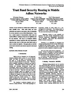
Figure 2: Path width for a distant s-d pair (7 hops away).

5

Numerical Simulations

We simulate the proposed ASWP algorithm over a 50-node network in a 2.5km×2.5km area. The transmission range of the nodes is 500m, and the interference range is 1km. The simulations demonstrate performance, complexity, and dynamics of the algorithm, discussed in the following sections respectively.

5.1

Performance

We compare the path width as we increase the load of the network. The load is represented by the average clique utilization, which is the average ratio of the used capacities over all cliques. We also consider the distance of the source-destination pairs, measured by the hop counts of the shortest path between the pairs. Intuitively, distant pairs seem to be more improvable, meaning that the widest path is wider than the shortest one. To see this in an opposite way, think of an one-hop pair: the shortest path is obviously the widest.

Due to the limit of space we present one figure (Figure 2) that shows the result for a 7-hops distant pair of nodes (chosen randomly). The Y-axis is the width of the best path between the pair. We plot this against rising utilization in the network. The figure shows, when k = 1, the proposed algorithm – denoted by ASWP(k = 1) – finds paths that are significantly wider than the shortest paths; k = 4 improves the path width very close to the optimum. For instance, when network utilization is 0.12, the path width of the shortest path is 357 Kb/s; ASWP(k = 1) improves

9

1 ASWP (k=1) ASWP (k=4) optimal ASWP

0.9

ratio of improved s/d pairs

0.8 0.7 0.6 0.5 0.4 0.3 0.2 0.1 0

1

2

3

4 5 6 7 distance between s/d pairs (Hop−count)

8

9

10

4 5 6 7 distance between s/d pairs (Hop−count)

8

9

10

26 ASWP (k=1) ASWP (k=4) optimal ASWP

average improvement (%)

24 22 20 18 16 14 12 10

1

2

3

Figure 3: The upper figure shows the ratio of the improved s-d pairs; the lower figure shows the average improvement. The results differentiate with respect to the hop distance. The load is medium (utilization = 0.32).

the value to be 416 Kb/s; And ASWP(k = 4) finds the optimal 488 Kb/s. The optimal value is computed using the centralized integer programming method.

When the load of the network increases, the improvements shrink. Indeed, when the utilization is over 0.53, there is no improvement at all. This can be explained by the fact that the network is so congested that none of the algorithms can find good paths. At this point, the widest available path is down to a few Kb/s.

The results are different for closer s-d pairs. Considering another randomly chosen s-d pair that are only 2 hops distant, at a high utilization of 0.53, we observe that the shortest path can carry only 15 Kb/s, while ASWP(k = 1) finds 143 Kb/s, and ASWP(k = 4) 222 Kb/s. To see this, note that the residual capacities vary significantly from clique to clique, especially when the load is high. For distant s-d pairs, there are always some congested cliques becoming the bottleneck, since paths traverse many cliques. But for close s-d pairs, it is sometimes possible to find paths that avoid the congested cliques. These paths can therefore be wider than the shortest ones.

Figure 3 evaluates the improvement over all s-d pairs in a medium-loaded network with utilization being 0.32. The

10

SP ASWP (k=1) ASWP (k=2) ASWP (k=4)

# of relaxation ops 12,900 14,293

running (sec) 5.3 27.9

16,146

50.4

22,032

80.0

time

Table 1: Time complexity for SP and ASWP algorithms.

figure compares the ASWP algorithm with the shortest path, and computes the width improvement from the width of the shortest path.

We first consider the percentage of s-d pairs whose path widths experience an improvement. Among all 2,450 s-d pairs of the 50-node network, 869 (35.5%) pairs achieves an improved width. The improvements depend on the distance between the s-d pairs. The upper figure of Figure 3 shows the ratio of the improvable s-d pairs increases as the hop distance increases.

A similar trend can be found in the lower figure, which presents the percentage improvement in the path width achieved by using ASWP. The values are percentage improvement over the width of the shortest paths, and are averaged over all the improvable pairs (clearly, there is no improvement for 1-hop pairs).

As k increases to a large enough value, ASWP is able to find the optimal path. Such a “large enough” k is bounded by the total number of paths in a graph, which grows exponentially with respect to graph size. For each s-d pair, we compute kopt , which is the minimal k for ASWP to find the optimal solution. Among all the s-d pairs, the largest kopt is 288. However, most pairs require a small kopt . Only 168 pairs require kopt > 4, accounting for 6.7% of all pairs. Consequently, applying ASWP(k = 4), we can find the optimum with the probability of 93.3%.

5.2

Time Complexity

The simulation results of the time complexity are summarized in Table 1. The first column shows how many times the relaxation operation is performed. The second column is the running time in seconds, which is a straightforward measure of the complexity. This is the case of computing path width for all s-d pairs in the medium loaded network. The algorithms are implemented and run in MATLAB 6.0 in a PC with 750 Mhz Pentium III.

11

We first focus on the ASWP algorithm and consider the impact of the k parameter. According to Table 1, ASWP(k = 2) sends 1.1 times more update messages than ASWP(k = 1), while ASWP(k = 4) sends 1.5 times more. These ratios are much less than the k values 2 and 4. However, ASWP with large k needs to compare and sort the records within the relaxation operations. We thus expect larger running time than the number of relaxation operations presents. According to the table, ASWP(k = 2) takes 1.8 times longer time than ASWP(k = 1), while ASWP(k = 4) is 2.9 times slower than ASWP(k = 1). These numbers show that ASWP scales sub-linearly as k increases. Note that these numbers do not include the time of computing the maximal cliques, since the clique computation is independent of k parameter. Table 1 also compare the time complexity between the ASWP algorithm and the Bellman-Ford shortest-path algorithm. The running time of ASWP with k = 1, 2 and 4 are about 5.3, 9.5 and 15.1 times slower than Bellman-Ford.

5.3

Dynamic Simulations

The simulations in the previous section demonstrate the performance by running ASWP on a network with a specific value of load. In this section, we want to show how ASWP behaves when flows are placed into the network dynamically, according to the path found by ASWP. We use the proposed algorithm to route an entire sequence of flow requests, and compare the performance generated over the same sequence of requests.

We choose five s-d pairs in the network, and generate fixed rate flow requests of 4 Kb/s. The requests come in at a rate of 0.32 flows per second, and are assigned uniformly to one of the five s-d pairs. If a flow is admitted, it will last a duration that is uniformly distributed between 400 and 2800 seconds. Thus on average the demand of the network is 0.32 ×

400+2800 2

× 4 = 2048 Kb/s, i.e., 2 Mb/s. We route the flows with SP and ASWP with k = 1, 2 and 4. Some

flows are admitted and installed accordingly, the others are rejected because the paths are not wide enough. Note that as the flows are installed, the network is utilized differently, since ASWP may find paths that are longer than the shortest paths.

The five s-d pairs are chosen randomly with distance consideration. Specifically, in the first column of Table 2, the five s-d pairs are randomly chosen from all the s-d pairs that are 2 hops distant. Similarly for the second and third rows, the s-d pairs are chosen with 4 hops and 7 hops distances respectively. In the last row, the distances between the s-d pairs are mixed, with 2, 3, 5, 6, and 7 hops each.

We run the simulation over 10,000 flow requests so as to compare the admission ratio in long run. Table 2 presents the

12

distance SP ASWP (k=1) ASWP (k=2) ASWP (k=4)

2 hops 99.4 100

4 hops 47.9 54.8

7 hops 31.8 44.1

mixed 66.5 71.4

100

54.8

43.4

71.0

100

54.7

43.9

70.9

Table 2: Admission ratio of SP and ASWP with different k in the dynamic simulations. The five s-d pairs are randomly chosen with distance consideration.

results: the ASWP algorithm consistently admits more flow requests than using shortest paths. The improvement varies for different s-d pair sets, and is up to 12.3% for the 7-hops pairs. Indeed, the improvements are more significant when fewer flows can be admitted into the network – a feature that augurs well for utilizing these algorithms in congested scenarios. The results demonstrate that ASWP is good at finding paths for flow requests between fixed s-d pairs.

We also observe that ASWP with k = 2 and 4 are not necessarily better than ASWP(k = 1) in the long run. As listed in Table 2, ASWP(k = 4) admits 0.5% less flows than ASWP(k = 1) in the mixed column, while ASWP(k = 2) admits 0.7% less flows than ASWP(k = 1) in the 7-hops case. The implication is that pursuing the widest paths may not gain in the long run. If the chosen paths are too long, they consume more network resources, and affect future requests. In short, it is beneficial to find wider paths than the shortest, but we must be cautious to employ the extremely long paths.

6

Conclusion

We study the problem of computing bandwidth guaranteed paths for given flow requests in an ad-hoc network. The problem is complicated because neighboring links share the medium. We use a conflict graph model to describe the interference. Applying the CG-based model, we construct the clique constraint as the feasibility condition of flows with bandwidth requirements. We then present the Ad-Hoc Shortest Widest Path (ASWP) problem as the mathematical abstraction that we want to solve.

We propose a distributed algorithm to solve the ASWP problem. Adopting the Bellman-Ford architecture and the k-shortest-path approach, the proposed algorithm is able to achieve a performance close to the optimum possible. Simulations evaluate the performance of the proposed algorithm, over various values of k.

13

The simulations offer another curious insight by looking at the dynamic behavior in the long term. It suggests that choosing wider paths is certainly better in a myopic sense, but may not be the optimal strategy for long-term performance. A small k value may provide the best tradeoff by computing less optimal but shorter paths.

References [1] R. Guerin, A. Orda and D. Williams, “QoS Routing Mechanisms and OSPF Extensions”, IETF Internet Draft, November 1996. [2] Z. Wang and J. Crowcroft, “Quality of service routing for supporting multimedia applications,” IEEE Journal on Selected Areas in Communications, vol. 14, pp. 1228-1234, Sept. 1996. [3] R. Gupta and J. Walrand, “Approximating Maximal Cliques in Ad-Hoc Networks”, Proceedings PIMRC 2004, Barcelona, Spain, September 2004. [4] H. Luo, S. Lu, and V. Bhargavan, “A New Model for Packet Scheduling in Multihop Wireless Networks”, Proceedings ACM Mobicom, pp. 76-86, 2000. [5] A. Puri, “Optimizing Traffic Flow in Fixed Wireless Networks”, Proceedings WCNC, 2002. [6] E. M. Royer, C. Perkins, and S. R. Das, “Quality of Service for Ad-Hoc On-Demand Distance Vector Routing,” Internet Draft draft-ietf-manet-aodvqos-00.txt, July 2000. [7] S. Chen and K. Nahrstedt, “Distributed quality-of-service routing in ad-hoc networks,” IEEE Journal Selected Areas in Communication, vol. 17 no. 8, pp. 1488-1505, Aug 1999. [8] C. R. Lin and J.-S. Liu, “QoS Routing in Ad Hoc Wireless Networks,” IEEE Journal on Selected Areas in Communications, vol. 17, no. 8, pp. 1426-1438, Nov./Dec. 1999. [9] C. R. Lin, “On-Demand QoS Routing in Multihop Mobile Networks,” Proceedings INFOCOM 2001, Anchorage, Alaska. [10] C. Zhu and M. S. Corson, “QoS Routing for Mobile Ad Hoc Networks,” Proceedings INFOCOM 2002, New York. [11] T. Salonidis and L. Tassiulas, “Distributed dynamic scheduling for end-to-end rate guarantees in wireless ad hoc networks,” submitted to publication. [12] Y. Yang and R. Kravets, “Contention-aware admission control for ad hoc networks,” UIUC Tech Report, 2003. 14

[13] Q. Xue and A. Ganz, “Ad hoc QoS on-demand routing (AQOR) in mobile ad hoc networks,” Journal of Parallel Distributed Computing vol. 63, pp. 154-165, 2003. [14] R. Rozovsky and P. R. Kumar, “SEEDEX: A MAC protocol for Ad Hoc Network,” Proceedings of The ACM Symposium on Mobile Ad Hoc Networking & Computing, Long Beach, California, 2001. [15] K. Jain, J. Padhye, V. N. Padmanabhan, and L. Qiu, “Impact of Interference on Multi-hop Wireless Network Performance,” Proceedings ACM Mobicom 2003, San Diego, CA, USA, September 2003. [16] M.R. Garey and D.S. Johnson, “Computers and Intractability: A Guide to the Theory of NP-Completeness”, W.H. Freeman and Company, New York, 1979. [17] R. Gupta, J. Walrand and O. Goldschmidt, “Maximal Cliques in Unit Disk Graphs: Polynomial Approximation”, Submitted to INOC 05. [18] R. Gupta, J. Musacchio and J. Walrand, “Sufficient Rate Constraints for QoS Flows in Ad-Hoc Networks”, Submitted to publication. Also available as UCB/ERL Technical Memorandum M04/42, Fall 2004. [19] S. Gerke and C. McDiarmid, “Graph Imperfection”, Journal of Combinatorial Theory, Series B, vol. 83, pp.58-78, 2001. [20] S. Sahni, “Computationally related problems”, SIAM J. Comput., vol. 3, no. 4, pp. 262-279, 1974.

15