Banker's Deadlock Avoidance Algorithm for

Banker’s Deadlock Avoidance Algorithm for Distributed Service-Oriented Architectures Matthew Martin† , Nicolas G. Grounds† , John K. Antonio‡ , Kelly Crawford† , Jason Madden† † RiskMetrics Group, 201 David L. Boren Blvd, Suite 300, Norman, OK, USA ‡ School of Computer Science, University of Oklahoma, Norman, OK, USA Abstract— A distributed service-oriented architecture comprises interconnected machines that together support a number of services. Concurrent service requests made to an individual machine are supported with shared, and limited, resources associated with that machine. A call to a service method may in turn invoke methods from other services, resulting in a nesting of service calls that is represented by a call tree. Deadlock occurs when a circular dependence is formed as a result of requests (calls) waiting for machine resources to be released by other requests. A deadlock avoidance technique is derived from Dijkstra’s Banker’s Algorithm that accepts or denies preferred scheduling and method-to-machine assignments proposed by underlying policies. Assumed to be known and available are estimates for the resource requirements of methods and the structures of the call trees. Simulation studies are conducted that demonstrate the effectiveness of the approach in avoiding deadlock, while not degrading (and in most cases improving) the performance of the underlying policies.

1. Introduction and Background Deadlock describes an undesirable phenomenon in which two or more processes hang indefinitely. Processes can enter the deadlock state—also known as the deadly embrace [1]—when each process is stalled because it is waiting for resources held by another process to be freed. For the case of two processes, deadlock occurs when the first process is waiting on the second process to free resources that the first process needs in order to proceed; however, the second process is also stalled because it is waiting for resources to be freed by the first. In general, deadlock can involve more than two processes; occurring when the resource requirements of the involved processes form a circular chain of dependencies with one another. Deadlock is a fundamental problem that has been studied extensively, often in the context of operating systems [2]. The seminal paper [3] defines four necessary conditions for the occurrence of deadlock. Even when these conditions are operative, it is generally not straightforward to determine if, or when, deadlock will occur. There are three broad approaches for dealing with deadlock: deadlock prevention; deadlock detection/recovery; and deadlock avoidance. The approach evaluated in the present

paper, which is the application of Dijkstra’s Banker’s Algorithm [1] in the context of a distributed service-oriented architecture (SOA), is characterized as a deadlock avoidance technique. For more discussion on the advantages that deadlock avoidance can have over deadlock prevention and detection/recovery approaches see [4]. In a distributed SOA [5], services define the different categories of computational operations that are available. Each service includes a number of associated service methods. Each machine in an SOA contains one or more service instances and must supply the resources necessary to carry out the methods associated with those instances. In general, machine resources include available memory, CPU capacity, persistent storage, I/O resources, network resources, and threads. The primary machine resources considered in the simulations conducted in the present paper are memory and CPU. The implementation of a given method may itself call upon other methods, and the called methods are not necessarily executed on the same machine as the calling method. Furthermore, method calls can be nested to an arbitrary depth; nested method calls are represented by a call tree. During the execution of a call tree, at most one method of the call tree is actively executing at a time; however, one or more methods may be in the holding state (i.e., waiting on the return from a called method). Executing methods consume both CPU an memory resources; holding methods consume memory. Concurrent execution of two or more call trees in a distributed SOA can lead to deadlock. An illustrative example of call trees deadlocking in an SOA is provided in [4]. The remainder of the paper is organized as follows. Section 2 provides a detailed description of the call tree execution model, including important state phasing definitions. The deadlock avoidance algorithm is developed in Section 3 and simulation studies are conducted in Section 4, followed by conclusions in the final section.

2. Call Tree Execution Model 2.1 Overview The execution of call tree T of Fig. 1 involves calls to six service methods, labeled a through e. A method is a sequence of one or more method segments; the boundaries

T

T

chain of segments a

a

b

a0

c

b

f

c

b0

f

a1 d

d

e

c0

e

d0 a

a a0

a1

b

a2 c

c0

b0

c1

a3

a0

b

a1

c0

c2

d

e

d0

e0

a3

f0

c1

c1 e0 f cf2

c

f

b0

a2

c2

d

e

a2

d0

e0

f0

assignable pre-assigned

b0 a1 c0 d0 c1 e0 c2

0

a3 assignable

chain of blocked ready executing completed blocked ready assigned executing completed segments (B) (R) (E) (C) (B) (R) (A) (E) (C) a0

pre-assigned

Fig. 1: Example call tree T and expanded view illustrating sequential ordering of its method segments.

between segments are defined where a method calls another method. Also shown in the figure is an expanded view of T , illustrating the sequential ordering in which the methods’ segments are interleaved. Thus, during execution of a call tree, at most one of its methods is executing at a time. Methods that do not call other methods are the singlesegment leaves of the tree, e.g., b0 , d0 , e0 , and f0 in the figure. The non-leaf methods (a and c in the figure) each include calls to other methods and thus are comprised of multiple segments. Once a method’s initial segment is assigned to a machine, it is assumed that its subsequent segments are pre-assigned to the same machine, i.e., method migration is not considered. Thus, the segments subsequent to the initial segment are shaded in Fig. 1 to indicate that their assignment is inherited from the assignment of the initial segment of the method.

2.2 Method Segment States Fig. 2 illustrates the sequential ordering (vertically) in which the chain of segments of call tree T of Fig. 1 are executed. The possible states of the segments are defined by the labeled columns: blocked (B); ready (R); executing (E); and completed (C). Upon initialization of call tree T , segment a0 transitions from blocked to ready, and all other segments remain blocked. After zero or more time units in the ready state, a0 is assigned to a machine (by some independent assignment policy) and begins executing, which is represented by a0 ’s transition from the ready state to the executing state.

a2 f0 a3

Fig. 2: Execution ordering of method segments of call tree T from Fig. 1 (shown vertically) with state transition diagram for each segment (shown horizontally).

Segment a0 stays in the executing state until the segment completes execution. The completed state is a terminal state for a segment. The dashed transition arc emanating from the completed state signifies that the completion of a segment triggers the next segment in the chain to transition out of the blocked state. This transition is associated with the transfer of control of execution when either a method calls another or when a method returns control back to its calling method. For the transition from a0 to b0 , note that b0 moves from blocked to ready upon a0 ’s completion. However, upon b0 ’s completion, the next segment, a1 , transitions directly from blocked to executing, bypassing the ready state. This is because a1 is pre-assigned according to a0 ’s assignment. Fig. 2 incudes the state transition diagram for the entire execution of T of Fig. 1. In general, a segment gi is in exactly one defined state at a time. Let σ(gi ) denote a mapping from a segment gi to a representation of its state. Making use of the abbreviations for the states provided in Fig. 2, the set of possible states for an initial segment g0 is defined by: σ(g0 ) ∈ {B, R, E, C}.

(1)

Similarly, the set of possible states for a subsequent segment gi , i > 0 is defined by: σ(gi ) ∈ {B, E, C}.

(2)

The R (ready) state is not a possible state for a subsequent segment because a subsequent segment inherits its assign-

ment from its associated initial segment; thus, it transitions directly from B to E. The total number of segments associated with a call tree is an important parameter, and shall be denoted by NT . For the call tree T of Fig. 1, NT = 11. In general, the value of NT is the sum of the number of vertices and edges in the call tree graph, which for T of Fig. 1 is NT = 6 + 5. The two time instances when each of the NT segments of a call tree begin executing, and complete executing, are important markers in defining life cycle phases of a call tree. Define tEi as the ith begin execution time marker for a call tree, which is the time instant when the ith segment of a call tree begins executing. Similarly, define tCi as the ith completion time marker for a call tree, which is the time instant when the ith segment of a call tree completes executing.

2.3 Method States In general, a method g can be in one of five possible states. Four of the states for a method g are named the same as the four possible states of a segment, i.e., {B, R, E, C}. The definitions for these states for method g follow logically from the states of g’s underlying segments. σ(g) = B ⇔ σ(g0 ) = B (3) σ(g) = R ⇔ σ(g0 ) = R

(4)

σ(g) = E ⇔ ∃i s.t. σ(gi ) = E

(5)

σ(g) = C ⇔ σ(gi ) = C, ∀i

(6)

In addition to the four states defined above, a method has another possible state called holding (H), defined as follows:  &  σ(g0 ) = C ∃i s.t. σ(gi ) 6= C & (7) σ(g) = H ⇔  σ(gi ) 6= E, ∀i > 0 Based on the definition of the holding state provided by Eq. 7, a method that is a leaf of a call tree can never be in the holding state. To show this, recall that a leaf method has only one segment, e.g., g0 . Thus, it is not possible for such a method to be in the holding state because it is not possible to satisfy the two conditions σ(g0 ) = C & σ(g0 ) 6= C, refer to Eq. 7. Fig. 3 illustrates the state transition diagrams for both non-leaf and leaf methods. For non-leaf methods, notice the presence of the cycle involving states E and H. The state transition for a leaf method contains no cycle; its transitions are the same as the initial segment transitions illustrated previously in Fig. 2. A method g that is in the executing state (i.e, σ(g) = E) is assumed to require both memory and CPU resources. A method g in the holding state (i.e., σ(g) = H) is assumed to require only memory resources. A method in a state other than E or H is assumed to have no resource requirement.

blocked (B)

ready (R)

executing holding completed (E) (H) (C)

non-leaf method leaf method

Fig. 3: State transition diagrams for non-leaf and leaf methblocked ready assigned executing holding completed ods. (B) (R) (A) (E) (H) (C)

2.4 Life Cycle Phases of a Call Tree non-leaf non-leaf Recall from Subsection 2.2 and that a call tree T has NT begin methods methods only execution time markersleafand NT completion time markers, which define time instances when each of the NT segments of a call tree begin complete respectively. blocked and ready assignedexecution, executing completed These markers are tEi and(E)tCi , and(C)are used (B) denoted (R) by (A) here in partitioning the time line of a call tree’s life cycle not holding into NT(H)+ 2 phases, numbered 0, 1, . . . , NT + 1. The ith phase of a call tree’s life cycle is denoted by φi and defined by holding (H)

 [0, tE1 ),     tEi , tEi+1 ), φi = [t  Ei , tCi ),   [tCi , ∞ ),

i=0 i ∈ {1, 2, . . . , NT − 1} i = NT i = NT + 1

(8)

Phases φi , i ∈ {1, 2, . . . , NT − 1}, can be further partitioned into two sub-phases called the ith primary sub-phase, denoted φ1i , and the ith secondary sub-phase, denoted φ2i : φ1i = [tEi , tCi ), i ∈ {1, 2, . . . , NT − 1}

(9)

 φ2i = tCi , tEi+1 ), i ∈ {1, 2, . . . , NT − 1}

(10)

From Eqs. 8 through 10, it follows that φi = φ1i ∪ φ2i , i ∈ {1, 2, . . . , NT − 1}

(11)

φ1i ∩ φ2i = ∅, i ∈ {1, 2, . . . , NT − 1}

(12)

and The primary sub-phase φ1i represents the time interval when segment i is executing. The secondary sub-phase φ2i represents the time interval after segment i has completed execution, but before segment i + 1 begins executing. Thus, φ2i represents a “delay” time in which neither segment i nor segment i + 1 is executing.

3. Deadlock Avoidance 3.1 Dijkstra’s Banker’s Algorithm The classic approach to deadlock avoidance in a resourceconstrained environment is Dijkstra’s Banker’s algorithm [1]. In the original formulation, Banker is assumed to have

control of a finite amount of capital (resource), which may be loaned to borrowers. Banker is responsible for accepting or denying (postponing) loan requests made by borrowers. Each borrower has a maximum loan limit, which bounds the total amount of capital each borrower may owe Banker at any instant. In addition to receiving loans, borrowers may pay back all or part of their outstanding loan balance to Banker. A key assumption is this: once a borrower’s loan amount reaches its maximum, the borrower will repay this amount back to Banker in finite time. Two example loan scenarios, one which is declared by Banker to be “safe” and the other “unsafe” are provided in [4].

3.2 Banker’s Algorithm for a Distributed SOA The Banker’s Algorithm is used here as a basis for avoiding deadlock when scheduling the execution of call trees in a distributed SOA. Assumed to be known to Banker is a phase number for each call tree and the requirements (e.g., memory and CPU) of the methods associated with the call trees. Having access to such information is realistic in the assumed environment in which off-line profiling and/or historical logging can be performed to collect/estimate these requirements. In this context, each call tree is a borrower of resources from the machines of the distributed SOA. As illustrated through the example presented in [4], deadlock can occur if too many methods from distinct call trees are allowed to advance their phase concurrently; but deadlock can be avoided if proper phasing (i.e., timing for the execution of the underlying methods) is employed. Unlike the implicit assumption of a centralized pool of resources—used to describe the original Banker’s Algorithm—the resources in an SOA are distributed across multiple machines. Thus, when applying Banker’s Algorithm in this context, an accounting must be made for the machine location(s) associated with available resources. Let Banker denote the implementation of the Banker’s Algorithm developed here for avoiding deadlock in a distributed SOA. In this context, Banker serves as a consultant to Advancer, which is the orchestration component of the system responsible for incrementing the phases of “advance-able” call trees in order to meet desired system objectives. Examples of such objectives might include maximizing throughput, minimizing latency, and/or minimizing tardiness. The role of Banker is to declare whether a proposed phase advancement is safe. In order to meet desired system objective(s), Advancer relies on an underlying SelectionPolicy module. Thus, Advancer first consults with SelectionPolicy to obtain a proposed phase advancement, and then consults with Banker to determine if it is safe to implement the (proposed) phase advancement. In its attempt to meet desired objectives, SelectionPolicy may propose the execution of many call trees concurrently and/or aggressively advance the phasing of many call trees, concurrently. Before com-

T: I:

set of all call trees current phasing; maps trees to phase numbers I : T → {0, 1, . . . , Nmax } where Nmax = max{NT : T ∈ T}

I∗ :

proposed phasing; maps trees to phase numbers

M:

set of machines where methods assigned to each M ∈ M are associated with current phasing I

M∗ :

set of machines where methods assigned to each M ∈ M∗ are associated with proposed phasing I∗

Fig. 4: Notation and definitions used by pseudocode of Fig. 5 Advancer(T, I, M) e ← {T ∈ T : TE 6= ∅} 1 T e 6= ∅) 2 while(T ∗ ∗ e I, M) 3 (T , g , M ∗ )← SelectionPolicy(T, ∗ 4 if(!M ) 5 break 6 I∗ ← I − {(T ∗ , I(T ∗ ))} + {(T ∗ , I(T ∗ ) + 1)} 7 M∗ ← update(g ∗ , M ∗ , M) 8 if(Banker(T, I∗ , M∗ )=SAFE) 9 I ← I∗ 10 M ← M∗ e ←T e − {T ∗ } 11 T Fig. 5: Banker used as a consultant by Advancer.

mitting to the proposed advancement, Advancer consults with Banker to determine safety. If Banker declares the proposed phasing to be UNSAFE, then Advancer again calls on upon SelectionPolicy to produce a modified phasing until one is determined that Banker declares to be SAFE. The interaction between Advancer, SelectionPolicy, and Banker is provided in Fig. 5. The notation and definitions used in the pseudocode of Fig. 5 are provided in Fig. 4. From Fig. 5 Advancer takes as input the set of call trees under consideration, along with their current phasing, and the set of machines. At line 1, a temporary set e is constructed containing all trees that do not have T a method executing; these represent trees that are eligible for phase advancement, i.e., they are advance-able. SelectionPolicy selects a tree, T ∗ , and a machine assignment, M ∗ , on which T ∗ ’s ready method g ∗ should execute (line 3). Assuming an assignment is made, a corresponding proposed phasing is constructed by incrementing the phase number of the selected tree (line 6). Likewise, the proposed states of the machines are updated by assigning ready method g ∗ to machine M ∗ (line 7). Banker is then consulted to determine safety of the proposed phasing and

... u

v

w

Fig. 6: Three-level aggregate tree structure associated with tree T of Fig. 1.

associated machine states. If safety is declared by Banker, then the proposed phasing and machine states are committed (lines 8 through 10). The selected tree T ∗ is removed from e (line 11) and execution continues until the temporary set T e T = ∅ (line 2) or SelectionPolicy does not return a machine assignment (lines 4 and 5). The pseudocode for Banker is provided in Fig. 7. Banker returns a value of either SAFE or UNSAFE. By returning SAFE, Banker asserts that given the call trees’ proposed phase numbers, there exists future scheduling phases to complete execution (without deadlock) of all call trees in T. By returning UNSAFE, Banker declares that continuing execution of call trees from their current state could lead to deadlock. Assumed to be known for each tree phase is a worst-case estimate of future resource requirements for executing the tree to completion. This estimate is modeled by an aggregate ∗ tree and denoted by A(T(I (T)) ). The depth of an aggregate tree equals the depth of the original tree and the number of methods comprising an aggregate tree equals its depth (i.e., it is a linear tree). For example, an aggregate tree associated with tree T of Fig. 1 has three methods and a depth of three. The resource requirements of each method of an aggregate tree equals the maximum resource requirements of methods yet to be completed at that level. Shown in Fig. 6 is the structure of the aggregate tree associated with tree T of Fig. 1. For phase 0 (before beginning execution of segment a0 ) the resource requirements of the associated aggregate tree are as follows: r(u) = r(a); r(v) = max{r(b), r(c), r(f )}; r(w) = max{r(d), r(e)}. For phase 3 (after completion of segment a1 and before beginning execution of c0 ) the resource requirements of the associated aggregate tree are as follows: r(u) = 0; r(v) = max{r(c), r(f )}; r(w) = max{r(d), r(e)}. From Fig. 7, Banker takes as input the set of call trees under consideration, along with their proposed phasing, and the set of machines with proposed method assignments. At b line 1, a temporary copy of T is constructed, denoted by T. For each tree, Banker determines if sufficient resources are available to satisfy future resource requirements for that tree. This is accomplished by employing SelectionPolicy to assign a machine to each method of the associated aggregate tree (lines 7 and 8). If all methods of the aggregate tree are

Banker(T, I∗ , M∗ ) b ←T 1 T b 6= ∅) 2 while(T 3 aTreeFits ← FALSE b 4 for(T ∈ T) 5 futurePhasesFit ← TRUE c ← M∗ 6 M ∗ 7 for(g ∈ A(T (I (T )) )) c 8 M ∗ ← SelectionPolicy({g}, 0, M) 9 if(!M ∗ ) 10 futurePhasesFit ← FALSE 11 break c ← update(g, M ∗ , M) c 12 M 13 if(futurePhasesFit) ∗ 14 M∗ ← release(T (I (T )) , M∗ ) 15 aTreeFits ← TRUE b ←T b − {T } 16 T 17 if(!aTreeFits) 18 return UNSAFE 19 return SAFE Fig. 7: Banker: Dijkstra’s Banker’s Algorithm for a distributed SOA.

assigned to a machine, then resources consumed by the tree b are released (line 14). Also, the tree is removed from T. b b Banker iterates over T until either: T is empty, in which case Banker returns SAFE (line 19) or all remaining trees’ future resource requirements cannot be satisfied in which case Banker returns UNSAFE (lines 17 and 18).

4. Simulation Studies 4.1 Overview The utility of Banker is evaluated through simulation studies. Two important objectives of the simulation studies are to determine: (1) the efficacy of Banker at avoiding deadlock and (2) the impact that Banker has on the behavior of SelectionPolicy with respect to a metric of system performance. Related to the first objective, a number of simulations are performed to verify that the use of Banker by Advancer does indeed prevent deadlock from occurring. For the second objective, special simulation realizations are identified (through trial and error) for which deadlock does not occur without the use of Banker. For each of these realizations, the performance obtained by SelectionPolicy is measured both with and without the consultancy of Banker. It is discovered that the use of Banker actually enhances performance for the case study and implementations of SelectionPolicy considered.

4.2 Simulation Environment The simulation environment employed models a real world SOA environment called BlueBox at RiskMetrics Group where clients submit their jobs to BlueBox in a number of different ways. In the actual system, these jobs are executed and the results are sent back to the clients. In the simulation environment, jobs are modeled as workflow graphs (WFGs), which are generated by a WFG generator. Associated with each WFG is a deadline that defines the point in time at which all computation for the WFG should be complete. The generated WFGs are one of three types: Interactive, Batch, or Webservice. During the simulation of a WFG’s execution, one or more of its trees have underlying methods that are ready and/or executing. These correspond to trees held in the set T as defined in Fig. 4, and used by Advancer (Fig. 5) and Banker (Fig. 7). The simulation environment also tracks tree phasing and corresponding methods assigned to each machine, referred to as I and M in Figs. 4 through 7.

 

Fig. 8: Time-line illustrating the three epochs for the case study.

ȕ

Ȗ1

Ȗ2

Ȗ

ȕ

Fig. 9: WFG structure used in simulations.

4.3 Selection Policies The simulation environment relies on Advancer to advance the phase of eligible trees in T. As shown in Fig. 5 Advancer relies on SelectionPolicy to make proposed machine assignments to ready methods. For the studies considered here, SelectionPolicy is composed of two steps. In the first step, ready methods associated with trees in T are prioritized. In the second step, ready methods are considered in priority order and assigned to machines with sufficient resources to satisfy resource requirements. A ready method is synonymous with a service request in an SOA and is referred to simply as a request for the remainder of the paper. The priority of requests is defined according to a request selection policy (RSP). The following four RSPs are evaluated: First Come First Serve (FCFS), Earliest Deadline First (EDF), Least Laxity First (LLF), and Proportional Least Laxity First (PLLF). The FCFS policy uses the value of the time instant that a WFG is generated to define the priority for all requests associated with the WFG. The EDF policy [6] prioritizes all requests of a WFG using the deadline associated with the WFG. The LLF policy [7], [6] prioritizes requests of a WFG according to their laxity, which is defined as the difference between the deadline of the WFG and the estimated finish time of the WFG. The PLLF policy [8] is an enhancement of the LLF policy that uses a “proportional” laxity value to prioritize ready requests of a WFG. The proportional laxity value is defined as the laxity value divided by the ideal execution of the WFG.

4.4 Case Study A case study is considered in which a single day is divided into three consecutive epochs. These three epochs are associated with WFG generation characteristics for a

typical operational business day. The first epoch is from time = 0 to time = 11 hours; the second epoch is from time = 11 to time = 12 hours; and the third epoch is from time = 12 to time = 24 hours (refer to Fig. 8). During the first and third epochs, only Interactive and Webservice WFGs are generated. During the second epoch, all three types of WFGs are generated. The first and third epochs represent periods of time before and after a relatively short epoch in which Batch WFGs arrive. The start and end times of the second epoch are defined by terms of servicelevel agreements (SLAs) related to timing of Batch WFG submission and execution. Typical terms of SLAs specify that daily Batch WFGs submitted within a specified time period will be completed by an agreed upon deadline. Fig. 9 shows the structure of the two-level WFGs assumed in the simulations. The WFG has two types of control nodes: parallel (meaning its children may be executed concurrently) and sequential (meaning its children must be executed in sequence). Call trees are the leaves of the WFG, represented with the triangular shapes. The root node is a sequential control node; the intermediate control nodes are parallel control nodes. In this figure, β is the number of parallel control nodes that are direct children of the root and are assumed to be sequentially executed. The notation γi represents the number of call trees associated with the ith parallel control node. The call trees of each parallel control node are assumed to be independent and may be executed concurrently. The values for β and γi vary for the three different WFG types. The parameter value ranges and distributions associated with the simulation studies are summarized in Table 1. The parallelization factor is needed in determining a base deadline for each generated WFG; it defines the degree of parallelism assumed for executing parallel call

Table 1: WFG parameter value ranges used for case study. Values in [Min, Max] sampled from uniform distribution. Parameter ∗ Inter-Arrival

Time (secs) β γi Parallelization Factor WFG Deadline Factor ∗ Poisson process.

Interactive WFG 60 [1, 1] [1, 2] 2 [1.1, 1.2]

Webservice WFG 120 [1, 3] [2, 3] 2 [1.3, 1.5]

Batch WFG 60 [3, 5] [5, 20] 2 [1.3, 1.5]

trees associated with a common control node. Once a base deadline is determined for a WFG, it is multiplied by the Deadline Factor (last row in the table) to define the actual deadline for the WFG. Interarrival times of the Interactive and Webservice WFGs are 60 seconds and 120 seconds respectively. The interarrival time of the Batch WFGs is assumed to be 60 seconds during the second time epoch from hour 11 to hour 12; Batch WFGs do not arrive outside this one-hour interval. For the simulations conducted, three call tree stuctures were considered for each WFG type. The structures for Interactive and Webservice WFGs are shown in Fig. 10. Likewise, Fig. 11 shows the structures for Batch WFGs. For a given WFG type, there is a uniform likelihood of selecting one of the three call tree structures.

Fig. 10: Call tree structures for Interactive and Webservice WFG types. Requests belonging to a call tree are assumed to have CPU and memory resource requirement values that depend upon the particular WFG type to which they belong. The ideal durations, CPU utilization factors, and memory requirements for the three WFG types are summarized in Table 2.

4.5 Results For the case study described in the previous subsection, one hundred simulations were conducted with the four RSPs described in Subsection 4.3. Each of the RSPs have different characteristics leading to different likelihoods for experiencing deadlock. Assuming Advancer does not utilize

Fig. 11: Call tree structures for Batch WFG types.

Table 2: Parameter value ranges for requests associated with call trees of Figs. 10 and 11. Request Parameter

Interactive WFG [1.0, 2.5] [0.5, 1.0] [0.05, 0.15]

Ideal Duration (secs) CPU Utilization Memory Usage 250

200

115 110 105 100 95 90 85 80 75

150

Webservice WFG [10.0, 50.0] [0.5, 1.0] [0.05, 0.10]

Batch WFG [50.0, 175.0] [0.5, 1.0] [0.05, 0.10]

Active Call Trees with Banker Active Call Trees without Banker

11

100

50

0

1

2

3

4

5

6

7

8

9 10 11 12 13 14 15 16 17 18 19 20 21 22 23 24 Hour

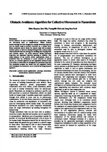
Fig. 12: Active call trees for PLLF with and without Banker for a case study realization in which deadlock does occur when Banker is not utilized.

Banker’s declaration of safety, the observed statistics for the occurrence of deadlock for each RSP were as follows: FCFS = 33%; EDF = 33%; LLF = 83%; and PLLF = 82%. A second set of simulations was conducted in which Banker’s declaration of safety was utilized. For this set of simulations, deadlock was avoided for all RSPs. As an illustration of how Banker interacts with the SelectionPolicy to avoid deadlock, consider Fig. 12. The figure shows the number of active call trees in the system for two simulations conducted, both employing PLLF as the RSP. In one simulation, Advancer utilizes Banker’s declarations of safety, and in the other it does not. From the figure, it is apparent that when the system is underloaded (hour one to hour eleven) Banker does not interfere with the scheduling decisions of SelectionPolicy. However, as resources become scarce, Banker begins to force SelectionPolicy to make only decisions that are SAFE. Just after hour eleven, large quantities of batch WFGs start arriving. When this occurs, more and more call trees become active. As illustrated by the inset portion of the figure, if decisions of SelectionPolicy go unchecked, deadlock occurs. In the simulation without Banker, deadlock is observed at the time instant where the graph ends. Also from inset portion of the figure, it is apparent precisely when Banker forces some active call trees to finish, thereby relieving memory pressure, before allowing more call trees

100

100

90 80

80

Percentage of Workflows

70 60

60

50 40

40

30 20

20

10 PLLF B-PLLF

0 -1

0

1

2

3

4

0 5

Normalized Tardiness

Fig. 13: Percentage of WFGs as a function of normalized tardiness for PLLF with and without Banker for a case study realization in which deadlock does not occur.

to begin executing. Banker delays the start/execution of certain call trees in order to ensure sufficient resources necessary for active call trees to complete. Because Banker sometimes forces SelectionPolicy to make decisions different than it would if it was running standalone, it follows that Banker has influence on the performance of SelectionPolicy in terms of tardiness relative to workflow deadlines. Interestingly, Banker does not negatively affect the performance of SelectionPolicy in terms of tardiness. In fact, in most cases considered, Banker actually improves the performance of SelectionPolicy. As an example of such a scenario, consider Fig. 13.

5. Conclusions A new deadlock avoidance algorithm, derived from Dijkstra’s Bankers Algorithm [1], is introduced for avoiding deadlock on a distributed SOA. The algorithm works by observing the current state of the resources in the system along with a worst case estimate of future resource requirements

and permitting the execution of only those call trees that will keep the system in a safe state. It is also worth noting that the algorithm takes a non-intrusive approach when the system resources are plentiful and does not influence the decisions of the underlying selection policy. The simulation results indicate that using Banker has multiple benefits. The selection policies considered in the simulations: FCFS, EDF, LLF, and PLLF have different characteristics leading to different likelihoods for experiencing deadlock. However, when Banker is utilized in tandem with any of the selection policies, deadlock is avoided. In addition to ensuring deadlock avoidance, Banker can influence SelectionPolicy to make decisions that improve the performance of the system in terms of workflow tardiness. One hypothesis is that the performance benefits observed when utilizing Banker are attributed to Banker forcing SelectionPolicy to concurrently execute different collections of call trees, prefering to run a larger number of shallow and/or undemanding call trees as opposed to a fewer number of deeply nested and/or resource intensive call trees.

References [1] W. Dijkstra, Edsger, Selected Writings on Computing: A Personal Perspective. Springer Verlag, 1982. [2] A. Silberschatz, Operating System Concepts. New York, NY, USA: John Wiley & Sons, Inc., 2007. [3] E. G. Coffman, M. Elphick, and A. Shoshani, “System deadlocks,” ACM Comput. Surv., vol. 3, no. 2, pp. 67–78, 1971. [4] M. Martin, Deadlock Avoidance in Distributed Service Oriented Architectures. Norman, OK: MS Thesis, University of Oklahoma, 2010. [5] M. P. Papazoglou and W.-J. Heuvel, “Service oriented architectures: approaches, technologies and research issues,” The VLDB Journal, vol. 16, no. 3, pp. 389–415, 2007. [6] V. Salmani, M. Naghibzadeh, A. Habibi, and H. Deldari, “Quantitative comparison of job-level dynamic scheduling policies in parallel realtime systems,” Proceedings TENCON, 2006 IEEE Region 10 Conference, November 2006. [7] S. H. Oh and S. M. Yang, “A modified least-laxity-first scheduling algorithm for real-time tasks,” Proceedings of the 5th International Workshop on Real-Time Computing Systems and Applications (RTCSA ’98), pp. 31–36, October 1998. [8] H. K. Shrestha, N. Grounds, J. Madden, M. Martin, J. K. Antonio, J. Sachs, J. Zuech, and C. Sanchez, “Scheduling workflows on a cluster of memory managed multicore machines,” Proceedings of the International Conference on Parallel and Distributed Processing Techniques and Applications (PDPTA ’09), July 2009.