Jun 13, 2010 - Peng Li, Kunal Agrawal, Jeremy Buhler, and Roger D. Chamberlain,. âDeadlock ...... [13] Arpith C. Jacob, Joseph M. Lancaster, Jeremy. Buhler ...
Deadlock Avoidance for Streaming Computations with Filtering
Peng Li Kunal Agrawal Jeremy Buhler Roger D. Chamberlain
Peng Li, Kunal Agrawal, Jeremy Buhler, and Roger D. Chamberlain, “Deadlock Avoidance for Streaming Computations with Filtering,” in Proc. of 22nd ACM Symposium on Parallelism in Algorithms and Architectures, June 2010, pp. 243-252.
Dept. of Computer Science and Engineering Washington University in St. Louis
Deadlock Avoidance for Streaming Computations with Filtering Peng Li
Kunal Agrawal
Jeremy Buhler
Roger D. Chamberlain
Dept. of Computer Science and Engineering Washington University in St. Louis St. Louis, MO 63130, USA
{pengli, kunal, jbuhler, roger}@wustl.edu ABSTRACT
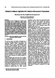
processing [25], molecular modeling [7], computational biology [13], and multimedia [15]. A streaming application is typically implemented as a network of computing nodes connected by unidirectional communication channels; we refer to such an implementation hereafter as a system. Abstractly, a system is a directed dataflow multigraph, with the node at the tail of each edge (channel) able to transmit data, in the form of one or more discrete tokens, to the node at its head. Figure 1a shows the dataflow graph of a small system. Compute node u, having no inputs, is a data source that can spontaneously generate tokens; v and w are intermediate nodes that operate on their single input streams; x, with no outputs, is a sink that computes some final result stream from two input streams. A realization of this system would map each node onto a physical computing resource in any way that permits the required topology of communication and has satisfactory performance.
The paradigm of computation on streaming data has received considerable recent attention. Streaming computations can be efficiently parallelized using systems of computing nodes organized in dataflow-like architectures. However, when these nodes have the ability to filter, or discard, some of their inputs, a system with finite buffering is vulnerable to deadlock. In this paper, we formalize a model of streaming computation systems with filtering, describe precisely the conditions under which such systems may deadlock, and propose provably correct mechanisms to avoid deadlock. Our approach relies on adding extra “dummy” tokens to the data streams and does not require global run-time coordination among nodes or dynamic resizing of buffers. This approach is particularly well-suited to preventing deadlock in distributed systems of diverse computing architectures, where global coordination or modification of buffer sizes may be difficult or impossible in practice.
Categories and Subject Descriptors C.2.4 [Computer-Communication Networks]: Distributed Systems—Distributed applications; D.1.3 [Programming Techniques]: Concurrent Programming—Distributed programming; F.1.2 [Computation by Abstract Devices]: Modes of Computation—Parallelism and concurrency
General Terms Figure 1: A streaming application example and a possible deadlock.
Algorithms, Design, Theory
Keywords Data Filtering, Dataflow, Architecturally Diverse Platforms
1.
INTRODUCTION
Streaming computation, a classic and still-popular computing paradigm, provides a convenient way to express high throughput-oriented parallel and pipelined computations. Application areas that use the streaming model include signal
Permission to make digital or hard copies of all or part of this work for personal or classroom use is granted without fee provided that copies are not made or distributed for profit or commercial advantage and that copies bear this notice and the full citation on the first page. To copy otherwise, to republish, to post on servers or to redistribute to lists, requires prior specific permission and/or a fee. SPAA’10, June 13–15, 2010, Thira, Santorini, Greece. Copyright 2010 ACM 978-1-4503-0079-7/10/06 ...$10.00.
243
This paper is largely motivated by our previous work on Auto-Pipe [4, 8], a compiler and infrastructure for mapping abstract systems of compute nodes onto diverse computing resources such as chip multiprocessors, reconfigurable logic, and graphics engines. Auto-Pipe does not support feedback loops in a system, so we will assume hereafter that the dataflow graphs of systems are directed acyclic multigraphs (DAMGs), which are most common in streaming applications. We study a streaming computation model in which tokens are indexed with non-negative integer timestamps. A data stream emitted by a node is a sequence of tokens with strictly increasing but not necessarily consecutive indices. For example, a source node might be a sensor that is occasionally triggered by some interesting event to emit a token containing data on that event along with the time at which it occurred. Streams have finite length; the last token in a
stream is always an End-Of-Stream (EOS) token with index ∞. Communication channels in our model are reliable and ordered, so that tokens emitted in index order can never be received out of order. However, a system provides no timing guarantees, so there may be an arbitrary finite delay before a token emitted onto a channel is received. Each channel uv can hold some fixed number of sent but not-yet-received tokens; this number is uv’s buffer size or capacity, denoted |uv|. Algorithm 1 describes how a node with an arbitrary number of input and output channels processes the streams of tokens on its inputs. A single computation can consume only input tokens with the same index ; at any time, a node’s current computation index is the index of the last set of inputs that it consumed. Computation on data with index i does not require that all input channels contain tokens with that index; it is well-defined even if only a subset of input channels ever receive tokens with index i. However, a node may not proceed to compute for index i unless it knows that no further tokens with this index will ever arrive at its inputs. A computation may output tokens with the same index as the inputs on any subset of a node’s outputs, including the empty set. We say that a computation filters an input on a channel q if it does not result in an output token on q. Filtering is a data-dependent behavior, performed independently by each node, that cannot be predicted at the time that a system is instantiated.
ure 1a, if node u generates inputs to both nodes v and w, v may emit output on channel vx, while w filters its inputs and emits nothing on wx. In this situation, node x is not able to consume the next token from vx because it does not know whether w will ever emit a corresponding token on wx. Because the system has bounded channel buffers, such blocking situations can lead to deadlock. For example, if channels uw and wx remain empty due to filtering while uv and vx fill, the system may reach the situation shown in Figure 1b. Node x is unable to consume data since it is waiting to receive data that must be sent from u, but u is unable to generate any more output because it is blocked trying to emit onto the full path from u to x. Hence, the system cannot make progress. Avoiding or remedying such deadlocks is an important consideration in system design. In this work, we describe how to prevent deadlock in streaming applications where some or all nodes may filter tokens. Because Auto-Pipe can map systems to a diverse, physically distributed array of computing devices, we have devised approaches that do not require global coordination among nodes, addition of new channels for control, or modification of channel buffer sizes. Instead, our approach augments data streams with extra dummy tokens — tokens that contain just an index but no data. These dummy tokens serve to inform downstream nodes that certain data items have been filtered and therefore the downstream node is allowed to proceed with its computation without waiting for these data items to appear. We present three algorithms for generating these dummy messages. The first algorithm is a rather naive and potentially inefficient algorithm based on the observation that a streaming application that has no filtering is not susceptible to deadlocks. Therefore, if a node sends a dummy message on a channel every time it filters a data item on that channel, then there is no possibility of deadlock. This approach may be good enough for some applications and has the advantage of being simple and not requiring any information about the buffer sizes on various channels. However, this algorithm may increase the channel traffic and it negates the advantage of filtering nodes. Our other two algorithms are more efficient in that they try to send fewer dummy messages than this naive algorithm by using information about buffer sizes. For both of these approaches, at compile time a dummy message interval is computed for each channel based on buffer sizes of downstream channels and dummy messages are sent at this interval. Since the buffer sizes (or at least a lower bound on them) are known at compile time and buffer sizes do not change during execution, this interval computation is a static overhead before the application starts running.
Algorithm 1: Single-node behavior in a system. ComputeIndex ← 0 ; while ComputeIndex 6= Index of EOS do if not source node then wait until every input channel has a pending token ; let T be minimum index of any pending token ; remove pending tokens with index T from input channels ; else T ← ComputeIndex + 1 ; ComputeIndex ← T ; perform computation on data tokens with index T ; if not sink node then emit output tokens with index T ; Computation on indexed token streams with filtering models applications that search their input streams for interesting events. For example, the popular bioinformatics search tool BLAST [2] may be viewed as a pipeline of compute nodes over a stream of DNA or protein sequence, in which each node identifies a progressively smaller subset of the stream as significant and filters away the rest. BLAST can be implemented as a linear pipeline, albeit with multiple channels between each successive pair of nodes. However, this paper generalizes to more complex computations with multiple data sources, such as an application to fuse data from an array of different environmental sensors. The filtering model is challenging in that dynamically determined stream rates make it hard to compute a feasible and efficient execution schedule at system compilation time. Moreover, filtering can cause some nodes in a system to block due to empty input channels. For example, in Fig-
2.
CONDITIONS FOR DEADLOCK
During a computing process, one node may be temporarily blocked by another due to an empty input or full output channel. However, not every blocking situation is a deadlock. In this section, we derive the conditions under which blocking can lead to deadlock. Definition 1. (Liveness) If a node can increase its compute index in finite time, we say the node is live, or equivalently that it makes progress. Definition 2. (Blocking Relation) If a node v is waiting for input from an upstream neighbor u, or if v is waiting to
244
send output to a downstream neighbor u because the channel buffer between them is full, we say that u blocks v, denoted u ⊣ v. If there exists a sequence of nodes v1 . . . vn such that vi ⊣ vi+1 for 1 ≤ i < n, we write v1 ⊣+ vn .
blockwise channels while uv and vx are counterblockwise channels. We notice that not all systems have deadlocks. For example, a system with just two nodes connected by one channel will never deadlock, even with filtering; the sender can block the receiver because the channel is empty, or the receiver can block the sender because the channel is full, but they cannot block each other at the same time. However, even quite simple systems, such as one with just two nodes connected by two parallel data channels, can deadlock.
Definition 3. (Deadlock) A system is said to deadlock if no node in the system is live but some channel in the system still retains unprocessed tokens (so that the computation is incomplete). We do not distinguish between local deadlock and global deadlock, as proposed in [10], because both of them will cause the computation not to complete. Now we prove that blocking cycle is a sufficient and necessary condition of deadlock.
Definition 5. (Potential Deadlock) A system with finite buffer sizes on all channels has a potential deadlock if, given the node topology and channel buffer sizes, there exist input streams and histories of filtering at each node such that a deadlock is possible.
Theorem 2.1 (Deadlock Theorem). A system eventually deadlocks if and only if, at some point in the computation, there exists a node u s.t. u ⊣+ u.
Definition 6. (Undirected Cycle) Given a system abstracted as a DAMG G, an undirected cycle of G is a cycle in the undirected graph G′ that is the same as G except that all edge directions have been removed.
Proof. (←) Suppose that at some point in the computation, there is a node u such that u ⊣+ u. Because a blocked node cannot make progress, no node on the cycle involving u can make progress. Hence, once the blocking cycle occurs, it will remain indefinitely. Moreover, not every pair of successive nodes in the cycle can be linked by an empty channel; otherwise, we would have that u is waiting for input from u, which is impossible because the graph of computing nodes is a DAMG. Hence, the blocking cycle contains at least one full channel, which means there are unprocessed tokens, and so the system is deadlocked. (→) Suppose that u ⊣+ u does not hold for any node u at any point in the computation. We show that, as long as there is any data in the system, some node is able to make progress; hence, the computation will never halt with unprocessed data on a channel. At any point in the computation, either every node with input data can make progress, or some such node u is blocked. Let H be the directed graph obtained by tracing all blocking relationships outward from u, such that there is an edge from v to w iff v ⊣ w. (H is also called a “waiting-for graph.” [6, 19]) By assumption, H has no cycles and is therefore a DAG. Let v0 be a topologically minimal node in H, which is not blocked by any node. If v0 has tokens on its input channels, it is able to consume them and so make progress. Otherwise, v0 ’s input channels are all empty, so that it cannot block any upstream neighbors. Moreover, since v0 itself is not blocked, either it is a source node that can advance its computation index by spontaneously producing tokens, or it must have received the EOS marker and so cannot block any downstream neighbors (which contradicts v0 ’s presence in H). Conclude that v0 is able to make progress, as desired.
For example, in the graph of Figure 1a, uvxw is an undirected cycle that can become blocking. We now show that in a general DAMG, every undirected cycle can become blocking. Theorem 2.2 (Potential Deadlock Theorem). Given a system S abstracted as a DAMG G, S has potential deadlocks if and only if G has an undirected cycle. Proof. (→) By definition, if S has a potential deadlock, then a deadlock can happen given the right pattern of inputs and filtering. By the Deadlock Theorem, such a deadlock implies the presence of a blocking cycle of nodes, which implies an undirected cycle of channels in G. (←) Suppose that there is an undirected cycle C of channels in G. We will construct a set of tokens and a filtering history that causes C to become a blocking cycle, implying a deadlock. First, we arbitrarily choose a direction on C to be the blockwise direction. We then topologically sort the nodes of the DAMG. We mark each channel and node with values calculated as follows. For each node u, if u is a sink node, Mu = 0; otherwise, Mu = maxuv Muv , where uv is any outbound channel from u. For each outbound channel uv, if uv is a counterblockwise channel in C, Muv = Mv + |uv| + 1; otherwise, Muv = Mv . The filtering history for each channel out of each node is as follows. Each input consumed by a node u results in output tokens (i.e. no filtering) on any output channel of u that is not on cycle C or is oriented counterblockwise on C. For an output channel uv that is oriented blockwise on C, u emits tokens on uv until its computation index reaches Muv , then filters (i.e. emits no output on uv) for any larger index. The above construction ensures that:
Definition 4. (Blockwise (not clockwise) and Counterblockwise) Let C be a cycle of blocked nodes v1 . . . vn , such that v1 ⊣+ vn and vn ⊣ v1 . The direction of increasing index on C is called blockwise, while the opposite direction is counterblockwise.
• For a blockwise channel uv in C, u ⊣ v because v will consume all Muv inputs sent to it by u, leaving the channel empty.
A channel on C between vi and vi+1 may be oriented either blockwise from vi to vi+1 or counterblockwise from vi+1 to vi . Because vi ⊣ vi+1 , a blockwise channel on a blocking cycle is always empty, while a counterblockwise channel is always full. For example, in Figure 1b, uw and wx are
• For a counterblockwise channel uv in C, v ⊣ u because u tries to send |uv| + 1 tokens to v after v becomes unable to consume tokens, and so uv becomes full and blocks further output by u.
245
Since each node in C now blocks its blockwise neighbor, it follows that for any node u in C, u ⊣+ u, which implies a deadlock.
Theorem 3.1 (Filtering Theorem). If no node ever filters any input, then the system cannot deadlock. Proof. The proof is by contradiction. Suppose there is a deadlock; then by the Deadlock Theorem, the computation reaches a state in which some node y ⊣+ y. Let C be the cycle of blocked nodes that includes y. Each node z on cycle C may be labeled with one of four types, depending on the directions of the channels that link z to its two neighbors in C:
The above proof shows that given enough input tokens and arbitrary filtering rules, any undirected cycle of G could cause a deadlock. In order to avoid deadlocks, we will enumerate these undirected cycles and schedule extra tokens for their channels so as to avoid the possibility of creating a blocking cycle.
3.
DEADLOCK AVOIDANCE ALGORITHMS
In our design of deadlock avoidance algorithms, we assume that at runtime, the nodes have no access to any dynamic global information. For example, a node u does not know whether any of the other nodes in the system are blocked. Our designs are based on the following objectives. First, we wish deadlock avoidance to be minimally intrusive on the nodes. That is, we do not want nodes to have to perform massive computations during runtime in order to prevent deadlocks. Second, we wish to make no modifications to the system’s communication topology. In particular, we do not want to add extra data or control channels; rather, we will avoid deadlock using only tokens sent on the existing data channels. Third, we do not wish to size channel buffers at runtime, since such reconfiguration is expensive and may not be possible if some channel buffer sizes are, e.g., determined by ASIC or FPGA hardware. In order to achieve these goals, we focus on designs that use static computations that can be performed at system construction time to configure the system such that no deadlocks will occur at runtime. In general, we cannot statically choose “large enough” channel capacities to avoid any possible deadlock; Buck [3] showed that it is undecidable whether an arbitrary dynamic dataflow computation remains within any particular channel capacity bound. We therefore augment the data streams between nodes by inserting additional tokens, called dummies, to limit the number of tokens that can remain unprocessed on any channel. A dummy is a distinguished class of token with an index but no content of its own. A dummy may be emitted as a standalone token, or it may be combined with a regular data token with the same index (such a data token may be said to have a “dummy flag” set). All compute nodes can recognize dummies, and a subset of nodes (to be specified) can generate them. The purpose of dummy tokens is to communicate a node’s current computation index to its descendants in the system, even if that node has not recently sent any data tokens.
3.1
1. Both channels are oriented blockwise, as for node w in Figure 1b; 2. Both channels are oriented counterblockwise, as for node v in Figure 1b; 3. The channel located to blockwise of z is oriented blockwise, while that to counterblockwise of z is oriented counterblockwise, as for node u in Figure 1b; 4. The channel located to blockwise of z is oriented counterblockwise, while that to counterblockwise of z is oriented blockwise, as for node x in Figure 1b. The rest of proof introduces the important concepts of minval and maxval, which will also be used in later proofs. Definition 7. (minval and maxval) For any full channel q, minval(q) is defined to be lowest index of any token queued on q, while maxval(q) is defined to be the highest such index. For an empty channel q ′ , minval(q ′ ) is defined to be the index of the token that has most recently traversed q′ . We now argue that, in the absence of filtering, the minval of a channel on C is always ≥ that of its counterblockwise neighbor. Let z be a node between two channels on the cycle. • If z has type 1, both channels are empty, with one pointing into z and one pointing out. Because z does not filter, every token input to z causes a token to be emitted; hence, the two channels have the same minval. • If z has type 2, both channels are full, with the blockwise channel pointing into z and other pointing out. Any value output by z has a strictly smaller index than a value waiting to be input to it, so the blockwise channel has the larger minval.
Using Dummies to Simulate Non-Filtering Computation
• If z has type 3, then both channels are outputs from z, and the blockwise channel is empty while the other is full. Because z does not filter, it always emits tokens with a given index on both channels at once. Hence, the minval of the blockwise channel is at least the index of the most recently emitted value on the other channel, which is ≥ the latter’s minval.
The simplest use of dummy tokens is as direct one-forone replacement of missing data: if a node u has an output channel q, and it performs a computation for index i that does not result in a data token being emitted on q, then it instead emits a dummy token on q with index i. Receiving a dummy token with index i on all inputs causes a node to perform a “null computation” and so to emit dummy tokens with index i on all outputs. This use of dummies, hereafter called the Naive Algorithm, simulates a computation in which no node ever filters its inputs. We claim that such a computation is immune from deadlocks.
• If z has type 4, then both channels are inputs to z, and the blockwise channel is full while the other is empty. The minval of the full channel must be strictly greater than that of the empty channel; otherwise, z could consume a value from the full channel.
246
Hence, the minvals of the channels in C increase monotonically to blockwise. Moreover, because there are no directed cycles in the original network, there is always a node of type 4 in C, and so the minvals of all channels in C cannot be identical. But this is impossible, because traversing the entire cycle implies that the minval of some channel is strictly greater than itself. Conclude that no blocking cycle can exist in the absence of filtering.
Algorithm 2: Single-node behavior with dummy propagation. ComputeIndex ← 0 ; foreach output port q do LastOutputIndexq ← 0 ; while ComputeIndex 6= Index of EOS do if not source node then wait until every input channel has a pending token ; let T be minimum index of any pending token ; consume pending tokens with index T from input channels ; else T ← ComputeIndex + 1 ; foreach output channel q do if T − LastOutputIndexq ≥ [q] OR some pending token with index T is a dummy then schedule a dummy token with index T for output q ; LastOutputIndexq ← T ; ComputeIndex ← T ; perform computation on data tokens with index T ; if not sink node then emit output tokens with index T , combined with any scheduled dummies ;
We extend the definitions of minval and maxval straightforwardly from a single channel to a directed path p composed of channels, provided that p is either completely full or completely empty. Hence, the minval of a full path p is the lowest index of any token queued on p, and so forth. The Naive Algorithm is straightforward but costly in terms of wasted channel bandwidth: the total number of tokens sent by the computation always equals the number of distinct computation indices times the number of channels. Real distributed computing systems have limited channel bandwidths, so that communication costs can become a bottleneck. In fact, for many applications, such as the BLAST application mentioned above, the primary purpose of most nodes is to filter the data stream. Using the Naive Algorithm for such applications would negate the communication bandwidth savings achieved by their natural filtering. Hence, we next give algorithms that reduce the number of dummy tokens sent while still ensuring that the resulting system is free from deadlock.
3.2
Algorithm 3: Dummy interval calculation with dummy propagation. Input: A system abstracted as graph G = {V, E} Output: Dummy intervals for each channel foreach edge uv ∈ E do [uv] ← ∞ ; foreach undirected cycle C of G do foreach node u with two output channels uv1 , uw1 on C do let p1 = uv1 . . . vm be maximal directed path on C starting with uv1 ; let p2 = uw1 . . . wn be maximal directed path on C starting with uw1 ; [uv1 ] ← min([uv1 ], |p2 |) ; [uw1 ] ← min([uw1 ], |p1 |) ;
Limiting the Frequency of Dummy Tokens
We now consider how to avoid emitting dummies for every data token filtered by a node. Our approach includes two parts. We first extend the behavior of each compute node u to include propagation of received dummy tokens, as well as generation of dummies on each output channel q of u at a statically defined dummy interval [q]. If [q] = ∞, then u never generates new dummies on output q; otherwise, it is guaranteed to emit a dummy each time its computation index advances by at least [q], which is computed by Algorithm 3. Using this extended behavior with the specified dummy intervals, we obtain a system that is deadlock-free yet sends many fewer dummies than the Naive Algorithm when some nodes filter their inputs. Algorithm 2 describes how we extend the behavior of a computation node to include generation and propagation of dummy tokens. Generator nodes are guaranteed to emit a dummy on channel q whenever the computation index has advanced by least [q] since the last dummy, regardless of whether any real output has been sent. All nodes propagate any incoming dummy token to all their output channels, combining it if needed with any data token with the same index to be emitted on each channel. Hence, even with dummies, no node ever emits two tokens with the same index on the same channel. This approach is referred as the “Propagation Algorithm” later. In the algorithm description and subsequently, |p| denotes the sum of all channel buffer sizes on a directed path p. A maximal directed path is one that is not a proper prefix of a longer directed path. Algorithm 3 iterates over all undirected cycles of the system, which may in general require time exponential in the system size; however, the algorithm is only run at system construction time and so does not impact runtime performance. For each node with two output channels on the same
undirected cycle, the algorithm calculates a dummy interval for each channel that (as we will prove) is small enough to guarantee that the cycle can never become blocking. Channels that are not the first channel on a directed path on some undirected cycle, including those not on a cycle at all, receive intervals of ∞. Theorem 3.2. If all nodes behave according to Algorithm 2, using the intervals calculated by Algorithm 3, then the system is deadlock-free. Proof. Suppose not; that is, suppose that the system as constructed above experiences a deadlock. According to the Deadlock Theorem, the system must at some point contain a blocking cycle C. We will show by contradiction that C cannot exist. Let C be given. Divide C into alternating maximal directed paths of blockwise and counterblockwise edges, as shown in Figure 2. Choose an arbitrary node with two output channels on C (as s1 in Figure 2) and, proceeding to
247
last [q] indices. Suppose that a data token was sent along pei from node si in the proof above; it could be filtered by any node on pei before reaching ri , thereby invalidating Inequality 3. Similarly, one cannot permit both a data token and a dummy token with a given index T to be sent separately, as doing so would invalidate Inequality 2. This scheme for deadlock avoidance can greatly reduce the frequency of dummy tokens on some channels in a system. In particular, a source node with two output channels q1 and q2 that emits a series of n tokens only on q1 would have to emit n dummy tokens under the Naive Algorithm but only about n/[q2 ] tokens with the revised approach. Unfortunately, propagation of dummy tokens ensures that a node receives all tokens (with distinct indices) emitted by any of its ancestors, even if the node is not on any of the cycles that required emitting the dummies in the first place! Hence, nodes with many ancestors that participate in undirected cycles may be flooded with useless dummy tokens. We can somewhat limit dummy propagation by noticing that, if we consider the communication links in our computing system as an undirected graph and segment this graph into its biconnected components, then every potentially blocking cycle is confined to a single biconnected component. Hence, it is not necessary to propagate dummies beyond the component in which they originate. We may compute biconnected components in time linear in the number of nodes and channels using Hopcroft and Tarjan’s algorithm [12], then label each channel with its biconnected component. A dummy arriving on some input channel q is then propagated only on output channels labeled with the same component as q.
blockwise from this node, label these paths in blockwise order as pe1 , pf 1 , . . . pek , pf k (“e” means “empty” while “f” means “full” here). By the Deadlock Theorem, each path pei consists entirely of empty channels, while each path pf i consists entirely of full channels.
Figure 2: The division of a blocking cycle for Theorem 3.2. For convenience, let pf 0 = pf k . Label each node between pei and pf i as the receiver ri , and label each node between pf (i−1) and pei as the sender si . Each sender node has two output channels on C, both of which receive finite dummy intervals according to Algorithm 3. The key observation is that, given the rules for assigning dummy intervals, node si cannot emit more than |pf (i−1) | tokens along path pf (i−1) without also sending a dummy token τ along path pei . Because path pf (i−1) is entirely full, while path pei is entirely empty, the dummy τ must have already been emitted by si and been propagated to receiver ri by the time the blocking cycle C formed. Recall the definitions of minval and maxval for paths as given in Section 3.1. Algorithm 2 and Algorithm 3 above imply that
3.2.1
Calculating Dummy Intervals Without Enumeration of the Cycles
Algorithm 3 for calculating dummy intervals requires enumerating every undirected cycle in G. While the algorithm could be carried out as written using a method for cycle enumeration [24, 17], this approach may do more work than necessary. In particular, suppose that for some node u with output channels uv1 and uw1 , the maximal directed path on a given cycle C starting with v1 is p1 . This path may also be maximal with respect to a large number of other cycles in G, whether through w1 or through another child of u. Enumerating all such cycles will not change the eventual minval(pei ) ≥ maxval(pf (i−1) ) − |pf (i−1) |. (1) dummy interval [uv1 ]. We can modify Algorithm 3 to interchange the order of Because each channel receives at most one token with a given its doubly-nested foreach loop: for each node u with two index, we have that, since pf i is full, output channels, consider all undirected cycles involving just maxval(pf (i−1) ) − |pf (i−1) | ≥ minval(pf (i−1) ). (2) these two channels. In fact, we need not actually enumerate all such cycles. Rather, for each channel uv1 out of u, it Finally, because the cycle C is a blocking cycle, ri remains is sufficient to enumerate directed paths p1 beginning with blocked by its counterblockwise neighbor even after receiving uv1 , then test whether each such p1 is maximal with respect dummy token τ . Hence, we have that to some (simple) undirected cycle involving node u. If so, minval(pf i ) > minval(pei ). (3) then we must set [uv1 ] ← min([uv1 ], |p1 |). The following connectivity test verifies whether a given Combining these three inequalities for a given i yields minval(pf i ) p1 is maximal with respect to some undirected simple cycle > minval(pf (i−1) ). But this inequality holds for every i, involving u. Suppose p1 ends with some vertex x. Delete and so we have transitively that minval(pf k ) > minval(pf 0 ), from G every vertex on p1 other than x, as well as all outwhich is impossible because these two paths are the same. going edges from x. Let G∗ be the undirected copy of the Hence, blocking cycle C cannot exist, and so deadlock is resulting graph. If there exists a simple path in G∗ connectimpossible. ing x to any other child w of u, then G has an undirected We note that in Algorithm 2, one cannot suppress a dummy simple cycle containing p1 that reaches u through edge uw. on a channel q even if a data token has been sent within the Moreover, the path p1 is maximal with respect to this cycle
248
because the path includes an edge that is into x in G. Conversely, if p1 is maximal for any simple cycle involving uv1 and some other uw, that cycle induces a path from x to w that is disjoint from the other vertices of p1 . The connectivity test for p1 can be implemented in time linear in |G| with any graph traversal algorithm. To avoid exploring paths that cannot lead back to another child of u in G, we may restrict the test to use only edges in the same biconnected component of G (properly, of its undirected copy) as the edge uv1 . Algorithm 4 shows the revised, non-cycle-enumerating algorithm for computing dummy intervals. Note that, for efficiency, the paths p1 should be enumerated in increasing order by length, so that the algorithm is finished with edge uv1 as soon as it discovers a cycle. Note also that each induced path from x to some other child w of u ends with some maximal directed path p2 starting with uw. As a further optimization, if the foreach loop over edges has not yet processed uw, we may set [uw] ← min([uw], |p2 |) to set an upper bound on the lengths of paths to explore for uw when its turn comes.
the new dummy interval computation assigns finite dummy intervals to all channels on the directed paths found by the previous algorithm, rather than just the first node. The assigned intervals are smaller than before for paths with two or more channels. As in the previous section, this algorithm may take exponential time, but it executes at configuration time and has no effect on the runtime of a computation. Also as in the previous section, we may replace the cycle enumeration of Algorithm 6 with the more efficient path enumeration and connectivity testing of Algorithm 4. Algorithm 5: Single-node behavior without dummy propagation. ComputeIndex ← 0 ; foreach output port q do LastOutputIndexq ← 0 ; while ComputeIndex 6= Index of EOS do if not source node then wait until every input channel has a pending token ; let T be minimum index of any pending token ; consume pending tokens with index T from input channels ; else T ← ComputeIndex + 1 ; ComputeIndex ← T ; perform computation on data tokens with index T ; foreach output channel q do if a data token with index T will be emitted on q then schedule a token with index T for output q ; LastOutputIndexq ← T ; else if T − LastOutputIndexq ≥ [q] then schedule a dummy token with index T for output q ; LastOutputIndexq ← T ; if not sink node then emit output tokens with index T , including any dummies;
Algorithm 4: Dummy interval calculation with propagation, no cycle enum. Input: A system abstracted as graph G = {V, E} Output: Dummy intervals for each channel foreach edge uv ∈ E do [uv] ← ∞ ; foreach node u with two output channels in the same biconnected component do foreach edge uv1 out of u do let G0 be the biconnected component of G containing uv1 ; foreach directed path p1 in G0 starting with edge uv1 do let x be the end vertex of path p1 ; G∗ ← G0 ; delete from G∗ all vertices on p1 except x ; delete from G∗ all outgoing edges from x ; if G∗ contains a simple undirected path from x to any child of u then [uv1 ] ← min([uv1 ], |p1 |) ;
3.3
Theorem 3.3. If all nodes behave according to Algorithm 5, using the intervals calculated by Algorithm 6, then the system cannot deadlock.
Eliminating Dummy Propagation
Proof. As before, suppose that a blocking cycle C occurs in a system using this deadlock avoidance scheme. Divide cycle C into paths, senders, and receivers as before. Label the nodes on path pei v0 , . . . vn , with v0 = si and vn = ri . Let γ = ⌈|pf (i−1) |/n⌉, the dummy interval defined for the channels on pei by Algorithm 6. We first prove that if ri has received no token with index minval(pf (i−1) ), then the last token received by node vj of pei must have index at most minval(pf (i−1) )+(γ −1)·(n−j). The proof is by induction on i in decreasing order. In the base case, when j = n, the lemma is trivially true, since vn = ri . For the inductive step, by the inductive hypothesis, the last token received by vj+1 had index at most Mj+1 = minval(pf (i−1) ) + (γ − 1) · (n − j − 1), and so vj ’s last token sent to vj+1 had index at most Mj+1 . Now suppose that vj has received a token with an index, say M ′ , greater than
In this section, we propose yet another deadlock avoidance scheme that uses a method similar to Algorithm 3 to assign dummy intervals to output channels. The key difference between the new scheme and that of the previous section is that dummy tokens no longer propagate. Since propagation is not required, we no longer need to send a dummy if we can send a data token with the same index; rather, the behavior at each node ensures only that some token is sent on channel q at least once each time the computation index increases by at least [q]. By increasing the frequency of dummy generation on some channels, we can guarantee freedom from deadlock without the need for dummy propagation. Hence this approach is referred as the “Non-Propagation Algorithm” later. Algorithm 5 describes node behavior in which dummies are never propagated beyond the channel on which they first appear, while Algorithm 6 gives a revised procedure to assign dummy intervals to channels. To avoid propagation,
Mj = minval(pf (i−1) ) + (γ − 1) · (n − j).
249
will still send dummy messages while the Non-Propagation algorithm will never send any dummy messages. Second, all downstream nodes propagate the dummy messages they receive. Therefore, in some cases, the dummy messages will be sent downstream even if they are no longer required. Due to these reasons, in most cases, we expect the Non-Propagation algorithm to be more efficient in terms of the number of dummy messages sent. Out preliminary empirical analysis confirms this intuition and we find that in our Mercury BLAST application, during one sequence search which had a filtering ratio greater than 95% and q = 1024, 72000 dummies were sent as a result of the Non-Propagation algorithm while this number would be 4 × 10⁸ if the Propagation algorithm was used. However, in theory, there are circumstances for which the Propagation algorithm will generate fewer dummy messages. Generally, this situation arises when the nodes filter a very large number of messages, sending virtually no real messages on some channels. Consider the following case. Let u1 u2 . . . uk+1 be some maximal path on an undirected cycle and the dummy interval for u1 u2 is q in the Propagation Algorithm. When the computation index increases from 0 to m at node u1 , in case of the Propagation Algorithm, u1 will send ⌊m/q⌋ dummies, which are then propagated by ui (1 < i ≤ k), so the total number of dummies is k∗⌊m/q⌋. According to Algorithm 6, in the Non-Propagation algorithm, the dummy interval for every channel on this path is at most ⌈q/k⌉. If all tokens are filtered by u1 , the total number of dummy messages sent by the Non-Propagation algorithm is about k ∗ ⌊m/⌈q/k⌉⌋, which is about k times larger than the number of messages sent by the Propagation algorithm.
Algorithm 6: Dummy interval calculation without dummy propagation. Input: A system abstracted as graph G = {V, E} Output: Dummy intervals for each channel foreach edge uv ∈ E do [uv] ← ∞ ; foreach undirected cycle C of G do foreach node u with two output channels uv1 , uw1 on C do let p1 = uv1 . . . vm be maximal directed path on C starting with uv1 ; let p2 = uw1 . . . wn be maximal directed path on C starting with uw1 ; [uv1 ] ← min([uv1 ], ⌈|p2 |/m⌉) ; for i in 2 . . . m do [vi−1 vi ] ← min([vi−1 vi ], ⌈|p2 |/m⌉) ; [uw1 ] ← min([uw1 ], ⌈|p1 |/n⌉) ; for i in 2 . . . n do [wi−1 wi ] ← min([wi−1 wi ], ⌈|p1 |/m⌉) ;
We have that Mj − Mj+1 = γ − 1, and so M ′ − Mj+1 ≥ γ, which means the interval between vj ’s last received and last sent tokens is at least γ. Algorithms 5 and 6 therefore ensure that vj must have sent a token, either real or dummy, to vj+1 with index > Mj+1 . But this contradicts our IH. Thus, we conclude that the last token received by vj has index at most Mj , as desired. Next, we observe a special case of the fact proved above: if ri has not received a token with index at least minval(pf (i−1) ), then si ’s most recently received token has some index T , where T
≤ < ≤
4.
minval(pf (i−1) ) + (γ − 1) · n minval(pf (i−1) ) + |pf (i−1) | maxval(pf (i−1) ).
But this is impossible because si has already emitted a token with index maxval(pf (i−1) ), so it must have received such a token. Conclude that minval(pei ) ≥ minval(pf (i−1) ). As in Theorem 3.2, we also have minval(pf i ) > minval(pei ) because cycle C is blocking, and so a contradiction follows using the cycle-following argument of that theorem. Hence, blocking cycle C cannot exist, and no deadlock occurs.
3.4
RELATED WORK
The streaming computation paradigm can be seen as an example of coarse-grained dataflow computing, which has two distinct domains: synchronous dataflow (SDF) [16] and dynamic dataflow (DDF) [3]. In SDF, data consumption and production rates are known at compile time, so we can compute a valid schedule statically to avoid deadlocks. In DDF, data rates are dynamic and cannot be known at compile time. Another issue of DDF is how to decide which data is consumed during one firing. Buck [3] used control switches to select the ports to read from and/or send to, which is called “Boolean Dataflow.” Prior to that, taggedtokens, similar to the ones we use, were proposed and implemented in the MIT Tagged-Token Dataflow Machine [22] and the Manchester Dataflow Computer [11]. Our computation model is similar to Kahn’s process networks (KPNs) [14]. A KPN consists of processes (we call them nodes) and unidirectional channels. The original KPN model has infinite channel buffers, which is impractical, so Parks et al. [23] introduced bounded memory models similar to the one we use. They also recognized that these networks have potential for deadlocks like the ones we study, which they call artificial deadlocks to distinguish them from deadlocks due to a directed cycle of empty channels. Deadlock treatment in distributed systems has been well studied. Chandy et al. developed algorithms to detect distributed deadlocks based on probes [6, 5]. Mitchell and Merritt designed a deadlock detection algorithm using public and private labels [19], which are similar to the notion of Chandy’s probe. After raising the issue of artificial deadlock in bounded KPNs, Parks tried to avoid such deadlocks by
A Comparison of Algorithms
In this section, we discuss the relative efficiency of the proposed algorithms in terms of the total number of dummy messages sent on all channels during the computation. Since the Naive Algorithm does not take advantage of channel buffers, it always sends more dummy messages than the other two algorithms. However, the Propagation and the Non-Propagation algorithms are incomparable; each may outperform the other based on the graph topology and buffer sizes. In most cases, we expect the Non-Propagation algorithm to perform better. Propagation algorithm has two inherent disadvantages over the Non-Propagation algorithm. First, it sends dummy messages at specific intervals regardless of whether the node is actually filtering any inputs. (Here we assume that the nodes are capable of filtering data, they just happen not to for that particular set of inputs.) Therefore, if no node ever filters any data, the Propagation algorithm
250
7.
dynamically increasing channel capacity. Geilen and Basten improved Parks’ idea and proposed a new scheduling algorithm which guarantees fairness and behaves correctly for bounded and effective KPNs [10]. Here “effective” means all tokens produced are ultimately consumed. This algorithm also requires dynamic changes to channel capacity. Nandy and Bussa claimed that runtime mechanisms could detect artificial deadlocks in bounded KPNs early [20], but deadlocks with multiple sources on blocking cycle were not identified in their work. Olson and Evans improved Mitchell’s algorithm to detect local deadlocks in bounded KPNs [21]. Later, Allen et al. from the same group proposed algorithms using private and public set to detect all deadlocks in bounded KPNs and to resolve them if possible [1]. However, not all detected deadlocks can be resolved. We note that all these deadlock avoidance and resolution algorithms require runtime change to channel capacities, while our algorithms do not. In our algorithms, we use dummy tokens to avoid deadlocks, inspired by null messages [9, 18] in parallel discreteevent simulation (PDES). In PDES, each message has a timestamp. To avoid deadlock, processes periodically send null messages, which contain only timestamps. These null messages let receivers advance their local clock values safely so that deadlocks are avoided.
5.
CONCLUSIONS AND FUTURE WORK
We have characterized deadlocks in our model of streaming computation with filtering nodes and have presented three deadlock avoidance algorithms under this model. Our techniques are provably effective, in that a system that uses them can never deadlock, and are lightweight in the sense that they do not require global control or extra communication channels and do not depend on dynamic buffer resizing. These are important considerations because we wish to apply our solutions to systems built with Auto-Pipe, which may utilize distributed, diverse computing resources that cannot easily be coordinated or modified at runtime. Our techniques require minimal infrastructural support, since dummy tokens use the existing communication channels, and our modifications to the behavior of nodes are minimal. There are several directions for future work. First, our algorithms for computing the dummy token intervals take exponential time. This drawback is not significant now since the computation occurs at configuration time and not at runtime, and the size of most graphs is relatively small. However, the size of graphs may increase in the future, and it would be useful to come up with polynomial time algorithms for computing or lower-bounding the dummy intervals. Second, we provide techniques for computing dummy intervals given buffer sizes. We would like to address the inverse problem where we statically size the buffers given that the system is willing to tolerate a certain dummy frequency. (Note that we are not talking about dynamic buffer resizing.) Third, we plan to implement our algorithms in Auto-Pipe and evaluate the performance impact of sending dummy tokens.
6.
REFERENCES
[1] G.E. Allen, P.E. Zucknick, and B.L. Evans. A distributed deadlock detection and resolution algorithm for process networks. In Proc. of IEEE Int’l Conf. Acoustics, Speech, Signal Processing (ICASSP), volume 2, pages 33–36, April 2007. [2] S. F. Altschul, T. L. Madden, A. A. Sch¨ affer, J. Zhang, Z. Zhang, W. Miller, and D. J. Lipman. Gapped BLAST and PSI-BLAST: a new generation of protein database search programs. Nucleic Acids Res, 25(17):3389–3402, 1997. [3] Joseph T. Buck. Scheduling Dynamic Dataflow Graphs with Bounded Memory Using the Token Flow Model. PhD thesis, University of California, Berkeley, 1993. [4] Roger D. Chamberlain, Mark A. Franklin, Eric J. Tyson, James H. Buckley, Jeremy Buhler, Greg Galloway, Saurabh Gayen, Michael Hall, E.F. Berkley Shands, and Naveen Singla. Auto-Pipe: Streaming applications on architecturally diverse systems. IEEE Computer, 43(3):42–49, March 2010. [5] K. Mani Chandy, Jayadev Misra, and Laura M. Haas. Distributed deadlock detection. ACM Trans. Comput. Syst., 1(2):144–156, 1983. [6] K. Many Chandy and Jayadev Misra. A distributed algorithm for detecting resource deadlocks in distributed systems. In PODC ’82: Proceedings of the First ACM SIGACT-SIGOPS Symposium on Principles of Distributed Computing, pages 157–164, New York, NY, USA, 1982. ACM. [7] Mattan Erez, Jung Ho Ahn, Ankit Garg, William J. Dally, and Eric Darve. Analysis and performance results of a molecular modeling application on Merrimac. In Proc. of ACM/IEEE Supercomputing Conference, Nov. 2004. [8] Mark A. Franklin, Eric J. Tyson, J. Buckley, Patrick Crowley, and John Maschmeyer. Auto-pipe and the X language: A pipeline design tool and description language. In Proc. of Int’l Parallel and Distributed Processing Symp., 2006. [9] Richard Fujimoto. Parallel discrete event simulation. Commun. ACM, 33(10):30–53, 1990. [10] Marc Geilen and Twan Basten. Requirements on the execution of Kahn process networks. In Proc. of the 12th European Symposium on Programming, ESOP 2003, pages 319–334. Springer Verlag, 2003. [11] J. R Gurd, C. C Kirkham, and I. Watson. The Manchester prototype dataflow computer. Commun. ACM, 28(1):34–52, 1985. [12] John Hopcroft and Robert Tarjan. Efficient algorithms for graph manipulation. Journal of the ACM, 16:372–378, 1973. [13] Arpith C. Jacob, Joseph M. Lancaster, Jeremy Buhler, Brandon Harris, and Roger D. Chamberlain. Mercury BLASTP: Accelerating protein sequence alignment. ACM Transactions on Reconfigurable Technology and Systems, 1(2), 2008. [14] Gilles Kahn. The semantics of simple language for parallel programming. In Proc. of IFIP Congress, pages 471–475, 1974. [15] Brucek Khailany, William J. Dally, Ujval J. Kapasi, Peter Mattson, Jinyung Namkoong, John D. Owens, Brian Towles, Andrew Chang, and Scott Rixner.
ACKNOWLEDGMENTS
This work was supported by NSF awards CNS-0751212 and CNS-0905368 and by NIH award R42 HG003225 (through BECS Technology, Inc.). R.D. Chamberlain is a principal in BECS Technology, Inc.
251
[16]
[17]
[18] [19]
[20]
Imagine: Media processing with streams. IEEE Micro, 21(2):35–46, March/April 2001. Edward A. Lee and David G. Messerschmitt. Synchronous data flow. Proceedings of the IEEE, 75(9):1235–1245, September 1987. Hongbo Liu and Jiaxin Wang. A new way to enumerate cycles in graph. In AICT-ICIW ’06: Proceedings of the Advanced Int’l Conference on Telecommunications and Int’l Conference on Internet and Web Applications and Services, pages 57–59, Washington, DC, USA, 2006. IEEE Computer Society. Jayadev Misra. Distributed discrete-event simulation. ACM Comput. Surv., 18(1):39–65, 1986. Don P. Mitchell and Michael J. Merritt. A distributed algorithm for deadlock detection and resolution. In PODC ’84: Proceedings of the Third Annual ACM Symposium on Principles of Distributed Computing, pages 282–284, New York, NY, USA, 1984. ACM. Bharath Nandy and Nagaraju Bussa. Artificial deadlock detection in process networks for eclipse. In Proc. of IEEE International Conference on Application-specific Systems, Architectures and Processors, pages 22–27, Washington, DC, USA, 2005. IEEE Computer Society.
[21] Alex G. Olson and Brian L. Evans. Deadlock detection for distributed process networks. In Proc. of IEEE Int’l Conf. Acoustics, Speech, Signal Processing (ICASSP), volume 5, pages v/73–v/76 Vol. 5, March 2005. [22] Gregory M. Papadopoulos and David E. Culler. Monsoon: an explicit token-store architecture. In Proc. of 17th Annual Int’l Symp. on Comp. Arch., pages 82–91, 1990. [23] Thomas M. Parks. Bounded Scheduling of Process Networks. PhD thesis, University of California, Berkeley, Dec 1995. [24] R. C. Read and R. E. Tarjan. Bounds on backtrack algorithms for listing cycles, paths, and spanning trees. Networks, 5:237–252, 1975. [25] Eric J. Tyson, James Buckley, Mark A. Franklin, and Roger D. Chamberlain. Acceleration of atmospheric Cherenkov telescope signal processing to real-time speed with the Auto-Pipe design system. Nuclear Instruments and Methods in Physics Research A, 585(2):474–479, October 2008.
252