Barycentric Interpolation and Exact Integration ...

Barycentric Interpolation and Exact Integration Formulas for the Finite Volume Element Method Tatiana V. Voitovich∗ and Stefan Vandewalle† ∗ †

Faculty of Engineering, Universidad Católica de Temuco, Manuel Montt 56, Temuco, Chile Department of Computer Science, Katholieke Universiteit Leuven, B-3001 Leuven, Belgium

Abstract. This contribution concerns with the construction of a simple and effective technology for the problem of exact integration of interpolation polynomials arising while discretizing partial differential equations by the finite volume element method on simplicial meshes. It is based on the element-wise representation of the local shape functions through barycentric coordinates (barycentric interpolation) and the introducing of classes of integration formulas for the exact integration of generic monomials of barycentric coordinates over the geometrical shapes defined by a barycentric dual mesh. We discuss especially a related problem of the approximation of the diffusion operators with spatially varying diffusion tensors, resulting in asymmetric stiffness matrices. Numerical examples are presented that illustrate the validity of the technology. Keywords: finite volume element method, barycentric coordinates, integration formulas. PACS: 47.11.-j, 47.11.Df, 02.60.Ed

INTRODUCTION Finite volume element (FVE) or box methods [2, 3, 4, 5], introduced by Baliga and Patankar as "control-volume finite element methods" in [1], play an important rôle in the present practice of numerically solving partial differential equations (PDEs). The finite volume element method was created to generalize and systematize the use of piecewise polynomial finite element spaces for discretization in the cell-vertex classical finite volume method, thus, one of the main features is the use of piecewise polynomial finite element spaces for the representation of the solution, the PDE coefficients and source functions. Another feature rooted in the finite element context is the suitability for use with unstructured grids, allowing the effective treatment of complex geometries, with a natural realization of local grid refinement and adaptivity. Alternative to the polynomial interpolation, for an accurate reconstruction of the fluxes, the recent FV schemes are so-called discrete duality finite volume methods (DDFV) combining cell-centered, cell-vertex FV integration and edge-based reconstruction of gradients (see [6] and references therein). On the other hand, the FVE method like all the finite volume methods employs the integral conservation form of the physical problem, thus (i) the method operates with the physically relevant quantities such as e.g. mass, momentum or heat flux, requiring in particular discrete conservation (ii) nonlinear analysis for the continuous model and analysis of convergence of the numerical scheme use the same techniques. The FVE method starts with a partitioning of the computational domain into a set of finite elements, and the subsequent definition of a dual finite volume mesh superimposed on the finite element grid. For every finite volume, the method writes out the integral conservation form of the PDE. Using the FE piecewise polynomial representation of the solution and PDE coefficients, a discrete set of linear or nonlinear equations is then constructed. In that step, one is faced with the integration of the element-based interpolation polynomials over certain geometrical shapes defined by the dual mesh. The present paper addresses the problem of the exact integration of those polynomials. Contrary to the finite element method, the technological basis of the FVE method is not well established; the integration formulas are in many cases not readily available. Such formulas are based on a local representation of the polynomials with the use of a set of basis functions and the subsequent exact integration of these basis functions over the corresponding geometrical shapes. In nodal finite element methods on simplicial grids, the polynomial basis functions ϕ (x, y) are usually expressed in terms of barycentric coordinates (in 2D also called area coordinates) Li : Ndo f

u(x, y) =

∑

i=1

ui ϕi (x, y) =

Ndo f

∑ uiϕi (L1 , L2 , L3 )

(1)

i=1

(here ui = u(xi ) denote the nodal value). Then, formulas for the exact integration of the generic monomials in

barycentric coordinates along an edge of a triangle, over a triangular element and over a tetrahedron, as provided, e.g., by Eisenberg and Malvern [7]: Z L

La1 Lb2 dL =

a! b! |L|, (a + b + 1)!

Z

La1 Lb2 Lc3 dA =

A

a! b! c! 2 |A|, (a + b + c + 2)!

Z

La1 Lb2 Lc3 Ld4 dV =

V

a! b! c! d! 6 |V |, (a + b + c + d + 3)!

(2) are used to complete approximation. Our aim is to derive similar formulas applicable to the FVE method, therefore, for the geometrical shapes determined by the dual mesh. Once derived, this formulas will provide a technological basis on which one can construct FVE solvers, in a similar way as (2) form the basis for the development of finite element solvers. Thus, as novel approach towards the derivation of FVE integration formulas, we will adopt the finite element practice to express the polynomial basis functions in terms of barycentric coordinates (barycentric interpolation), see (1). An alternative general approach for the integration of polynomial basis functions over arbitrary polygonal and polyhedral grids was given by Liu and Vinokur [8] and results in the exact integration of monomials in Cartesian coordinates.

EXACT INTEGRATION OF POLYNOMIALS USING BARYCENTRIC COORDINATES The FVE method is applicable to a wide range of PDEs. Here, for illustration purposes, we focus on a 2D convectiondiffusion-reaction equation from fluid dynamics, of the form

∂ (ρ u) + ∇ · (ρ vu − λ ∇u) + γ u = fu in ΩT = Ω × (0, T ) , ∂t

(3)

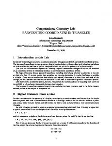
where ΩT = Ω×(0, T ) is the space time cylinder, with Ω a bounded domain, subject to initial and boundary conditions; ρ is the fluid density, v is the velocity vector, λ is the diffusion coefficient, and fu is the volumetric source of u. Let T denote a conforming triangulation of Ω such that the intersection of the closures of two distinct triangles is either empty or consists of one common vertex or edge. For each node xi a polygon Ωi is constructed on the centroids of the triangles and the mid-points of the edges that constitute a partition of Ω called barycentric dual mesh (see Fig.1, left). ˜ k denote barycentric subdomains of a simplex, In 3D also the barycenters of the tetrahedron sides are involved. Let Ω let Sk denote a dual median segment emanating from node k (Fig 1(a)), and Skl denote a dual quadrilateral that lies on the median plane coming out of edge connecting nodes k and l (Fig. 2(a)). For the representation of the FVE solution, spatially varying PDE coefficients and source functions, on T we consider the usual finite element space of continuous piecewise polynomial functions o n ¯ | v |T ∈ P1 ∀ T ∈ T h , (4) Sh = v ∈ C0 (Ω) where P1 is the space of first degree polynomials in two variables. Which integrals arise? Consider an element T ∈ T . Remind that barycentric coordinates Li are a kind of local coordinates in a simplex such that any point in the simplex is given by

∑ Li = 1.

r = ∑ Li ri ,

3

3

~ 3 T2

S2

~ 1 1

(5)

i

i

S3 T3

a

~ 2

=

L1 (x; y )

n12 n21

T1

S1

z

n31 n13

n32 n23

2 1

2

y

l2

1

x

l2

b

x

l1

y

l1

y

3

S2 S1

2 x

FIGURE 1. Fragment of the primary and dual grid (left); key notations used in the text (center); the barycentric coordinate L1 , L1 = ψ1 (x, y)(right).

We use the barycentric coordinates both to perform the nodal interpolation (1) and to derive the integrals arising in the approximation of the FVE integral conservation form of the IBVP. The advantage lies in that the barycentric coordinates are natural for the simplexes therefore resulting in shorter, rotationally symmetric and more "transparent" formulas; morover, the scheme is essentially the same in two and three space dimensions. An example of barycentric interpolation is the approximation of the diffusion flux Jνdk in assumption that the spatially varying coefficient λ (x) is approximated by conforming linear finite elements (4) with local shape functions denotes as ψˆ m (x):   Z  3  3 3 3 λ (x) = ∑ λm ψˆ m (x) = ∑ λm Lm x ∈ T, J˜νdk = − ∑ λm Lm ds ∑ (k2l nν k,x + k3l nν k,y )ul on Sk . (6) m=1  l=1 m=1 i=1 Sk

Note that to complete the approximation (6) one should introduce formulas for the integation of Lm over Sk , allowing simple geometrical interpretation (see Fig.1, right). Generally, the following integrals appear while approximating convection and diffusion fluxes, source, reaction terms, unsteady terms, and boundary conditions: Z

Z

La1 Lb2 Lc3 ds,

La1 Lb2 ds,

(7)

Γ∩∂ Ωi

˜k Ω

Sk

Z

La1 Lb2 Lc3 dΩ,

the integration of the generic monomials in barycentric coordinates over dual mesh median segments, over barycentric subdomains and over boundary edges segments, respectively (k = 1, 2, 3). How to evaluate them? A prerequisite for the evaluation of the integrals are the formulas relating the barycentric coordinates with themselves on the elements of the dual mesh. Evaluation of the line/surface integrals (2D/3D) is performed with the use of the following. •

•

•

parametrization of the dual mesh median segments/dual mesh quadrilateral parts of the median planes, using (5) resulting, e.g. in 1 r = L1 r1 + L2 r2 + (1 − L1 − L2 ) (r3 + r4 ) , on S12 (3D); (8) 2 calculation of the differential element resulting e.g. in (see Fig. 2(b)): ∂r ∂ r × dL1 dL2 = 12 |S12| dL1 dL2 , on S12 (3D). (9) dS = ∂ L1 ∂ L2

writing the general form of the integral allowing its easy evaluation for any (a, b, c, d), and formulation of a general rule for the monomials of a certain order, resulting, e. g., in 1

Z

S12

La1 Lb2 Lc3 Ld4 dS

12 |S12| = c+d 2

Z4

dL1

1−1L 3Z 3 1

1

La1 Lb2 (1 − L1 − L2 )c+d dL2 +

12 |S12| 2c+d

0

0

Z3 1 4

dL1

1−3L Z 1

La1 Lb2 (1 − L1 − L2 )c+d dL2 . (10)

0

Evaluating of the general form for the area and volume integrals requires in addition consideration of lines/surfices of equal order of coordinates Li to find the integration limits as functions of the barycentric coordinates. V1

V1

(2)

r1

S12 V2

V2

(1)

P34

a

r2

T1 b

FIGURE 2. A median plane, emanating from edge E12 , and quadrilateral part S12 ; surface parametrization: partial derivatives of (1) (2) the position vector r1 = ∂ r/∂ L1 , r2 = ∂ r/∂ L2 (right).

0.01

y, m 0 0

0.5

0

0.5

0

0.5

0

0.5

0

0.5

0

0.5

0

0.5

0

0.5

0

0.5

0

0.5

0

0.5

u, m/s

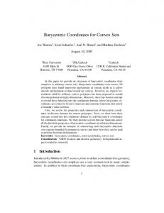
FIGURE 3. Laminar flow over a backward-facing step. Experimental and calculated velocity profiles for Re=389 at different locations; ⋄ experiment Armaly et al. [10], – FVE/FLOM solution.

What are the relevant cases? As the p-refinement in the FVE method requires introduction of additional sets of the dual meshes, which in the case of systems could lead to that some important conservation properties are violated, the relevant cases are the monomials of low order. Thus, for the integration over dual mesh lines one has:

Z

Sk

Lν ds =

(

1 6 5 12

|Sk |

if ν = k,

|Sk |

if ν 6= k.

Z

Lν Lµ ds =

Sk

      

1 27

|Sk |

if ν = µ = k,

7 108 |Sk |

if ν 6= µ and ( ν = k or µ = k )

19 108 |Sk |

otherwise.

(11)

where k = 1, 2, 3. For a detailed evaluation of the integrals and their values for the relevant cases we refer to [9].

NUMERICAL EXPERIMENTS Laminar flow over a backward-facing step.

The model is given by the incompressible Navier-Stokes equations

∂ (ρ u) ∂ρ + ∇ · (ρ u ⊗ u − τ ) = −∇p + f , + ∇ · (ρ u) = 0, in ΩT , (12) ∂t ∂t u is the velocity vector, p is the pressure, τ is the viscous shear stress tensor, ρ is the density. The modeling is done with the use of collocated equal order interpolation for the pressure and velocity as the unknown fields; the special PrakashPatankar interpolation of the velocity components in the continuity equation is used in order to prevent checkerboard pressure fields; the SIMPLER scheme is applied as the overall solution scheme. Steady state longitudinal velocity profiles, computed with the flow-oriented modified upwind scheme are presented in Fig. 3. The close match with the data from paper [10] is obvious. The triangulation consisted of 1594 nodes, with a refinement near the walls and the separation line. The reattachment point calculated with the use of the modified flow-oriented upwind scheme [11] is given by the value 7.813S. This is in excellent agreement with the experimental value of 7.81S. A similar computation with the mass-weighted upwind scheme gives the less accurate result 7.217S.

REFERENCES 1. 2. 3. 4. 5. 6. 7. 8. 9. 10. 11.

B. R. Baliga and S. V. Patankar, Numer. Heat Transfer 3, 393–409 (1980). R. E. Bank, and D. J. Rose, SIAM J. Numer. Anal. 24, 777-787 (1987). W. Hackbusch, Computing, 41, 277–296 (1989). Z. Cai, J. Mandel, S. McCormick, SIAM J. Numer. Anal. 38, 392-402 (1991). S. F. McCormick, Multilevel Adaptive Methods for Partial Differential Equations, SIAM, Philadelphia, 1989. B. Andreianov, F. Boyer, F. Hubert, Num. Meth. PDE 23, 145–195 (2007). M. A. Eisenberg, L. E. Malvern, Int. J. Numer. Methods Eng. 7, 574-575 (1973). Y. Liu, M. Vinokur, J. Comput. Phys. 140, 122-148 (1998). T. V. Voitovich and S. Vandewalle, Num. Meth. PDE 23, 1059–1082 (2007). B. Armaly, F. Durst, J. C. F. Pereira, and B. Schoening J. Fluid. Mech. 127, 473–496 (1983). E. P. Shurina, O. P. Solonenko, T. V. Voitovich, Computational Techologies, 7 98-120 (2002).