IEEE TRANS. VISUALIZATION AND COMPUTER GRAPHICS, VOL. X, NO. Y, ZZZZZ XXXX
1
Bas-Relief Generation Using Adaptive Histogram Equalisation Xianfang Sun, Paul L. Rosin, Ralph R. Martin, and Frank C. Langbein, Member, IEEE
Abstract—An algorithm is presented to automatically generate bas-reliefs based on adaptive histogram equalisation (AHE), starting from an input height field. A mesh model may alternatively be provided, in which case a height field is first created via orthogonal or perspective projection. The height field is regularly gridded and treated as an image, enabling a modified AHE method to be used to generate a bas-relief with a user-chosen height range. We modify the original imagecontrast-enhancement AHE method to also use gradient weights, to enhance the shape features of the bas-relief. To effectively compress the height field, we limit the height-dependent scaling factors used to compute relative height variations in the output from height variations in the input; this prevents any height differences from having too great an effect. Results of AHE over different neighbourhood sizes are averaged to preserve information at different scales in the resulting bas-relief. Compared to previous approaches, the proposed algorithm is simple and yet largely preserves original shape features. Experiments show that our results are in general comparable to and in some cases better than the best previously published methods. Index Terms—Bas-relief, adaptive histogram equalisation, feature enhancement.
I. I NTRODUCTION Bas-relief sculpting is a technique which has been practised for thousands of years. The idea is straightforward: a flattened sculpture is produced on some base surface—for example, portraiture on coinage. The overall range of depth of the elements in the sculpture is highly compressed. Parallel or perspective viewing effects may also be used. Bas-reliefs usually have a single z depth for each x-y position, and portions of the scene nearest to the viewer are elevated most [1]. The production of bas-reliefs is currently a costly and timeconsuming process, requiring skilled sculptors and engravers. Automatic capture of computer models of 3D shape is becoming more commonplace using 3D scanners. This provides a foundation for automation in bas-relief making, resulting in reduced costs, and shorter time-to-market. Such advantages also allow bas-reliefs to be extended to a wider range of application areas such as packaging, where traditionally the costs or lead times have often been too high. However, current commercial CAD tools for bas-relief work, such as Delcam’s ArtCAM, cannot yet be considered to provide a full solution to relief making. X. Sun is with the School of Computer Science, Cardiff University, 5 The Parade, Cardiff CF24 3AA, UK, and the School of Automation Science and Electrical Engineering, Beihang University, Beijing 100191, P. R. China. Email:
[email protected]. P. L. Rosin, R. R. Martin, and F. C. Langbein are with the School of Computer Science, Cardiff University, 5 The Parade, Cardiff CF24 3AA, UK. E-mail: {Paul.Rosin, Ralph.Martin, F.C.Langbein}@cs.cardiff.ac.uk. Manuscript received XXXX.
Of course, considerable artistic skills are needed to decide upon the composition and view of the subject matter. Having chosen these, however, simple experimentation shows that an acceptable bas-relief cannot be made by linearly compressing a 3D scene’s depth coordinates while preserving width and height (see Fig. 1(b)). In principle, by suitably choosing the direction of the light source, and the surface albedo, the image of a bas-relief generated by an affine transformation of the 3D surface can be indistinguishable from that of the original 3D surface [2]. However, in most cases, it is not possible to control the light source, surface albedo and viewpoint. Considerably more sophisticated methods are needed to produce a bas-relief which has the right kind of visual appearance [3]–[6]. The academic work to date has considered the issue of how to achieve the necessary compression of depths, and even so, has not achieved entirely satisfactory results. The next section summarises state-of-the-art approaches. We then present a new depth compression method based on an adaptive histogram equalisation (AHE) method taken from image processing, which has been adapted to bas-relief production. Our goal is a simple method for bas-relief generation which clearly preserves visible shape details in the final results, as demonstrated in Fig. 1(c). II. P REVIOUS W ORK Relatively little academic literature to date has considered the automatic production of bas-reliefs. One older paper [1] gives a basic approach to the problem, while two recently published papers independently devised rather similar, more sophisticated, solutions [4], [6]. The earliest paper [1] treats bas-relief generation as a problem of embossing on the view plane. The key principle used is that depth within the relief should be a function of the distance between the observer and any projected point. The authors expect this function to preserve linearity, and note that standard perspective transformation has the required properties. Thus, they compress z coordinates inversely with distance, while also adding perspective in x and y if desired. Their results are generally of the correct nature, but of unacceptable quality in detail. For example, a bas-relief of a head gives undue prominence to the hair, while other reliefs may look rather flat. The authors note that good results can only be obtained if the artist subtly edits the 3D model before applying their approach. However, they state an important principle for generating basreliefs: unused depth intervals at height discontinuities should be removed (either manually or automatically) to make best use of the allowed bas-relief depth.
IEEE TRANS. VISUALIZATION AND COMPUTER GRAPHICS, VOL. X, NO. Y, ZZZZZ XXXX
(a) Fig. 1.
(b)
2
(c)
3D dragon model (a) and the bas-reliefs generated by simply scaling depths (b) and our method (c).
More recent papers [4], [6], [7] note a similarity between bas-relief generation and high dynamic range (HDR) imaging, in which multiple photographs of the same scene over a wide range of intensities, are composited and displayed on an ordinary monitor: the range of intensities must be compressed in such a way as to retain detail in both shadows and highlights. In relief processing, depths replace the intensities in HDR. However, it is not straightforward to apply these ideas. As [6] notes, some HDR methods are global, e.g. histogram equalisation (HE) [8], while others apply similar methods to local regions of the image [9]. The latter generally make better use of the dynamic range, and are necessary if unused depth intervals at height discontinuities are to be removed locally. HDR methods often separate the image into frequency components and attenuate the low frequencies; one consequent problem which must be avoided is ringing. For a recent overview of HDR imaging methods, readers are referred to [10]. Weyrich et al. [6] used HDR-based ideas to give a mostly automatic method for constructing bas-reliefs from 3D models; they also imposed some additional requirements, such as maintaining small, fixed-size depth discontinuities. Their method uses perspective foreshortening as in [1] as a first step, but unlike that paper, subsequent steps do not preserve planarity. Instead, emphasis is placed on retaining important visual clues: steps at silhouettes, and surface gradient directions (but not magnitudes). This method allows user-controlled attenuation of low frequencies in gradient space; relief shape is then recovered by integrating the gradient field in a least-squares sense. The goal is to make an orthogonal view of the relief, seen with a particular camera, similar to the appearance of the original object; viewing off-axis leads to distortion and a flat appearance. This approach also automatically removes unused depth intervals. The authors usefully give a set of principles for constructing reliefs, taken from the artistic literature. These cover: how to generate the illusion of depth, object ordering, depth compression, depth discontinuities, steps, and undercuts. They also note that material properties are important, and that specular reflections can look larger on reliefs than on the original object. Independently, [4] uses different steps to generate reliefs, but actually performs rather similar computations in terms of the underlying principles. 3D shape is first represented
in differential coordinates. Unsharp masking and smoothing are combined to emphasise salient features and de-emphasise others. The shape is then scaled in differential coordinates, and finally the bas-relief is reconstructed from these differential coordinates. Again, a chosen viewing direction is taken into account. The authors note that their approach leads to a certain amount of distortion, and that it does not enhance the silhouette of the shape (unlike [6]). They suggest shading exaggeration as a possibility for future research. A related paper [7] considers feature-preserving depthcompression of range images, based on linear rescaling of the gradient of the image, again using unsharp masking for gradient enhancement. The results of this approach unnaturally exaggerate areas with high gradient but flatten areas with low gradient, and thus look rather flat. An improvement on this method is proposed in [5], which rescales the gradient nonlinearly using a function from [9], providing a compromise between the exaggerated and the flattened areas. In summary, these papers produce results which at first sight appear acceptable, but reveal shortcomings under more critical analysis. In [4] and [7], the impression of curvature is lost, and in [5], the silhouettes of shapes are not well preserved, while in [6], a bump appears to exist in the foremost rod where rodshaped features cross (see Fig. 9). There is clear scope for improved methods of depth compression for relief making. An extensive literature exists on image enhancement [11], some of which is clearly applicable to bas-relief production. Even within a single application area, however, there is no single image enhancement algorithm that is consistently the most effective. One of the most commonly used techniques is unsharp masking, whose application to bas-relief generation we have already noted. It essentially enhances edges by increasing the magnitude of high frequency components. One drawback as a consequence is that it magnifies any noise present in the image. Moreover, it enhances high contrast areas more than low contrast areas, leading to undesirable artifacts when low contrast areas must also be enhanced. Modified versions of unsharp masking have been developed to overcome these limitations [12]. The relation of histogram equalisation to HDR imaging has been noted, together with its limitations as a global method. As a result, adaptive histogram equalisation (AHE) utilising local windows has been considered, e.g. [13]. However, win-
IEEE TRANS. VISUALIZATION AND COMPUTER GRAPHICS, VOL. X, NO. Y, ZZZZZ XXXX
dow size and other parameters need to be carefully chosen, otherwise, again, noise may be enhanced and undesirable artifacts created [14]. Most work in this area does not take into account the properties of the human visual system. Of the few exceptions, Frei [15] suggested use of a hyperbolic rather than constant intensity histogram, based on Weber’s law: perceptual brightness is a logarithmic function of intensity. Further work in this direction is given in [16], [17]. However, such perceptually-based optimisation is not directly applicable to depth modifications for relief making: these do not correspond directly to intensities. Many other approaches to contrast enhancement have also been proposed. E.g., Subr et al. [18] pose the problem as optimisation of a scalar function measuring local contrast in the image, subject to constraints on local gradients and intensity ranges; they also refer to other approaches based on anisotropic diffusion, morphological techniques, clustering, retinex theory, k-sigma clipping, and curvelet transformations. For consumer electronics, several HE methods have been proposed having a brightness-preserving property, such as bi-HE [19], [20], multi-HE [21], equal-area dualistic subimage HE [22], brightness-preserving HE with maximum entropy [23], and brightness-preserving dynamic HE [24]. Inspired by the close relations between HDR, HE and basrelief generation, we consider a local version of HE in this paper. We modify AHE [13] for use for depth compression in providing automated bas-relief generation. III. P ROBLEM S TATEMENT AND A PPROACH As a bas-relief typically has no undercut, it can be represented by a height field (measured in z direction), which for simplicity of processing we take to be regularly gridded in x and y at a sufficiently fine resolution. Thus, as a starting point, we take a gridded height field representing a scene containing one or more objects. Cignoni et al. [1] and Weyrich et al. [6] list several features of bas-reliefs, and requirements that height fields must fulfil in order to suitably represent a bas-relief. While a bas-relief typically has much smaller z extent than x or y extent, it should still exhibit shape features as clearly as possible, so that it is visually close to the original input shape when viewed in the z direction from the front. In practice, this means that the height field should exhibit strong contrast or significant variation in shading (typically due to variation in slope) where objects or parts of objects meet. If the input is a 3D (mesh or CAD) model, we thus need to first generate a height field from it, using a suitable view. Following Cignoni et al. [1], we do so by retrieving depth values from a z-buffer following perspective projection of the 3D model. The depth values, lying in [0, 1], may be simply read from an OpenGL z-buffer as suggested in [6]. ¿From the input height field, we wish to generate an output height field meeting the bas-relief requirements. The user also either states a desired final range of z values, or, amounting to the same thing, the overall compression factor to be achieved in z direction: the ratio of the distance between lowest and highest points in the height field before and after processing. A
3
non-linear depth compression process is then used to adapt the height field to meet this requirement while preserving shape features. In the next section, we give our approach to this depth compression problem. IV. D EPTH C OMPRESSION Histogram equalisation (HE) methods can enhance contrast in image processing. We use such methods to produce enhanced features in the final compressed height field. The standard HE method is simple but is unsuitable for our problem, because it uses a single monotonic function to transform the entire image, and does not consider local intensity distributions. Instead, we use a local or adaptive HE method [13], and modify it to enhance the depth compression effect. Before performing AHE, we automatically remove unused depth intervals between the background and the scene, as suggested by Cignoni et al. [1]. We detect the corresponding smallest and second smallest height values, and move the scene towards the background, so that the second smallest height value is now the same as the smallest. A. Height Field Histogram Equalisation We next introduce our notation and describe the standard HE method in the context of height fields rather than intensity images. The goal of HE is to apply a non-linear monotonic transformation to the input image intensities such that the resulting image has a uniform intensity distribution. Doing so maximises the entropy of the data, and as a consequence improves the overall image contrast. We suppose the input to be a height field z(x, y) with M × N uniformly gridded sample points S = {(x, y) : x = 1, . . . , M, y = 1, . . . , N }. Suppose the minimum and maximum of z(x, y) are zmin and zmax , respectively. The height values of the sample points are placed into B equalsized bins {bi : i = 1, . . . , B} between zmin and zmax , giving a histogram H = {hi : i = 1, . . . , B}, where hi is the number of points whose height value falls into the ith bin, defined by bi = [zmin + (i − 1)δ, zmin + iδ) for i = 1, . . . , B − 1, and δ = (zmax − zmin )/B. Note that bB = [zmax − δ, zmax ]. The cumulative histogram C is defined as X ci = hj . (1) j≤i
The histogram equalisation process maps the height values in each bin to new values such that the new histogram is (approximately) uniformly distributed. The new height z 0 (x, y) for a sample point z(x, y) ∈ bi is given by ci − c1 0 0 0 (z − zmin ) + zmin , (2) z 0 (x, y) = zi0 = cB − c1 max 0 0 where zmin and zmax are the desired minimum and maximum height values after HE. Note that in image processing, often 0 0 the output intensity range Imax −Imin is larger than Imax −Imin to maximise contrast in the final result, whereas here we want a smaller range of heights to produce a bas-relief. Typically, 0 we set zmin = 0 for simplicity of computation. Note that z(x, y) is (at least in principle) a continuous value, but z 0 (x, y) is discrete. Because of this, the new
IEEE TRANS. VISUALIZATION AND COMPUTER GRAPHICS, VOL. X, NO. Y, ZZZZZ XXXX
equalised histogram is not exactly uniformly distributed with equal numbers of points z 0 (x, y) in each bin. The uniformity achieved is dependent on the number of bins B. The larger B, the higher the uniformity, and the fewer the artifacts caused by discretisation, but at the expense of increased computational effort. We have used B = 10000 in all of our examples with max(M, N ) ranging from 624 to 1024. Experiments showed that the artifacts are negligible for B this large, although they become noticeable in all of our examples if we reduce B to 3000. Combining Equations (1) and (2), we obtain 0 ∆zi0 = zi0 − zi−1 =
0 zmax
0 zmin
− cB − c1
hi .
(3)
This implies that the larger hi , the larger the height difference 0 ∆zi0 between successive height values zi0 and zi−1 . Because the output height range is fixed, Equation (3) means that HE increases contrast, i.e. the difference in height, for bins with high counts, and decreases it for bins with low counts, thus enhancing global contrast. In some sense then, enhancement of global contrast implies enhancement of global shape features of the height field, which is a desirable property for depth compression. However, because HE focuses on global features, local features may be lost, and shape distortion may also result. In the next section, we thus use adaptive histogram equalisation to tackle the problem of local shape distortion. ¿From Equation (3) we can also see that if hi = 0, then 0 zi0 − zi−1 = 0. This means that HE will effectively discard depth intervals of the original height field containing no sample points. Doing so is desirable in any depth compression method, as it ensures optimal use of the limited depth range available in the output—depths with no sample points are simply skipped. Unlike the methods of Kerber et al. [5], [7] and Weyrich et al. [6] where gradients are set to zero when they are over a threshold, which locally collapses large steps, HE compresses global steps no matter whether these steps are large or small, and no thresholding is needed. Nevertheless, when we consider the depth intervals between the background and the foreground, we can see that although large steps are removed, the depth difference between the background and the foreground in the resulting bas-relief may still be rather large if the number of points in the second non-empty bin (which contains foreground points nearest to the background) is large, which occurs in many cases. This is also why we move the scene towards the background as a preprocessing step. Because no local information is used, standard HE is less effective at dealing with local steps. Adaptive HE as introduced in the next section uses local information to compress local steps. B. Adaptive Histogram Equalisation with Gradient Weights In this section, we introduce AHE [25] and explain how it deals with local features. We then present a gradient-weighted AHE method to provide improved depth compression results. AHE is also called local HE. For each point (or pixel, in terms of image processing), it performs HE within a local neighbourhood of this point, and uses the result as the output
4
value for the point. Let N (x, y) = {(u, v) ∈ S : |u − x| ≤ m, |v − y| ≤ m} be the m-neighbourhood of point (x, y), and let hi (x, y) be the number of points in N (x, y) whose height value falls into bi . We compute the local cumulative histogram using X ci (x, y) = hj (x, y). (4) j≤i
If point (x, y) falls into the ith bin bi , then the new height value z 0 (x, y) = zi0 (x, y) at point (x, y) is calculated by zi0 (x, y) =
ci (x, y) − c1 (x, y) 0 0 0 (z − zmin ) + zmin . cB (x, y) − c1 (x, y) max
(5)
Note that the only difference between Equation (2) and (5) is that the former uses the global cumulative histogram while the latter uses the local one. Because of this difference, AHE can efficiently compress local steps. Its ability to do this depends on the size m of the neighbourhood: as m increases, the method becomes less efficient. In the extreme case when m = max(M, N ), AHE is equivalent to standard HE. However, it is not necessarily true that, the smaller m, the better the method compresses local steps. As m is reduced, the total number of points in N (x, y) becomes smaller, and if it is too small, many hi (x, y) may be zero. If this happens, the local histogram after equalisation will be far from uniform, and the resulting effects of feature enhancement will be unsatisfactory: ultimately, too small a value of m results in distortion of the output height field. For example, in an extreme case, suppose i > 1 and all neighbouring points of (x, y) fall into the same bin i. Then cB (x, y) = ci (x, y), and the output height at (x, y) 0 , whatever the original z(x, y), even if it will be set to zmax were close to zmin . Since AHE can efficiently compress local height variations with relatively small m and global height variations with large m, we perform AHE with different sizes of m and take the average of the resulting height fields as the final result. In this way, we can compress both local and global steps, and preserve different scales of information in the resulting bas-relief. Fig. 2 shows part of a bas-relief computed using different m, and an average. Look carefully at the front wall of the tower. It appears bumpy in differing places as m varies; such problems are much less visible in the averaged bas-relief. Even though AHE can compress height fields better than standard HE, it is still not perfect. Because both standard HE and AHE only use the histogram (i.e. the proportion of samples falling into each bin), but not any shape information, it is incapable of preserving shape features such as the surface gradient. The latter is important as it determines the surface’s brightness under given lighting conditions. Hence, we introduce the novel idea of applying gradient weighting to AHE, to preserve relative magnitudes of gradients in the output height field. The difference between gradient-weighted AHE and unmodified AHE lies in the computation of hi (x, y). A simple gradient-weighted scheme would replace the computation of
IEEE TRANS. VISUALIZATION AND COMPUTER GRAPHICS, VOL. X, NO. Y, ZZZZZ XXXX
5
(a)
(b)
(c)
(d)
(e)
(f)
Fig. 2. Zooms of bas-reliefs showing part of a building produced by AHE with different neighbourhood sizes: m = 16, 32, 64, 128, 256 from (a) to (e), and the average of these bas-reliefs (f).
hi (x, y) by hi (x, y) =
X
g(u, v),
(6)
(u,v)∈N (x,y); z(u,v)∈bi
where the weight g(u, v) is the gradient magnitude computed using the Sobel operator [11]: q g(u, v) = gx2 (u, v) + gy2 (u, v); (7) here
where α is a parameter set between 0.5 and 10 as suggested in [6]. This function has the property of strongly attenuating large gradients while preserving small gradients, and thus preserving small shape details in the modified AHE procedure. Note that α = 0 implies the identity function T (g(u, v)) = g(u, v). We also suggest that the influence of neighbouring points on the local histogram should decrease as their distance from the central point grows. To do so, we use a Gaussian distance weighting function: 2
gx (u, v) = z(u − 1, v − 1) + 2z(u − 1, v) + z(u − 1, v + 1)− z(u + 1, v − 1) − 2z(u + 1, v) − z(u + 1, v + 1),
(8)
gy (u, v) = z(u − 1, v − 1) + 2z(u, v − 1) + z(u + 1, v − 1)− z(u − 1, v + 1) − 2z(u, v + 1) − z(u + 1, v + 1).
(9)
Unmodified (unweighted) local histograms would be computed by simply setting g(u, v) = 1 in Equation (6). The idea behind Equation (6) is that, the larger the gradients of points in bin bi , the larger hi (x, y), and thus, from Equation (3), the larger the height difference ∆zi0 (x, y). Because larger gradients in the original height field result in larger height changes, the introduction of gradient weights in AHE helps to preserve the original gradient information in the resulting height field. We may further improve results slightly by using an idea due to Weyrich et al. [6]: we apply a non-linear transformation to the gradient magnitudes before use (see Fig. 4). This nonlinear transformation is defined as 1 (10) T (g(u, v)) = log (1 + α g(u, v)), α
D(d(u, v)) = e−d(u,v) /2m , (11) p (x − u)2 + (y − v)2 is the distance bewhere d(u, v) = tween the central point (x, y) and the point (u, v) in the m-neighbourhood. We use a Gaussian function as we want the influence of boundary points of the neighbourhood to be very small, such that moving the central point does not change the local histogram dramatically. This reduces height artifacts even if points at the boundary change substantially in adjacent neighbourhoods. While [13] also considered weighted AHE for image processing, using a conical weighting function, they found little noticeable difference in results compared to unmodified AHE in their tests, and thus did not recommend its use. However, in our case, experiments show that this Gaussian weighting function generally improves the results. Combining gradient weighting with non-linear compression of gradient magnitudes, and distance weighting, gives the final form we use for the gradient-weighted histogram: X hi (x, y) = T (g(u, v))D(d(u, v)). (12) (u,v)∈N (x,y);z(u,v)∈bi
After computing this gradient-weighted hi (x, y), we again use Equations (4) and (5) to calculate the new height value for a
IEEE TRANS. VISUALIZATION AND COMPUTER GRAPHICS, VOL. X, NO. Y, ZZZZZ XXXX
single gradient-weighted AHE. C. Limitations on Height-Dependent Scaling Factors As the total height range is fixed for the output height field, HE increases the height difference (i.e. the height contrast) between certain adjacent height values and decreases others (see Section IV-A). From Equation (3) we can see that if hi is great for a certain i, the height difference between zi0 and 0 zi−1 will be great. If this is too great, problems can arise: many other i will correspond to small height differences. The result can be both, shape distortion, and enhancement of any noise present in the original height field. To limit the contrast in an AHE approach for image enhancement, Pizer et al. [13] suggest modifying the local histograms so that no hi (x, y) exceeds a given limit. Larson et al. [8] suggests the same modification for standard (global) HE. We follow this idea and modify the local gradient weighted histogram in the same way. In detail, Pizer et al. [13] clip the excess bin contents of hi (x, y) over a given limit and redistribute the clipped contents among other histogram bins. They considered two schemes of redistribution. One uniformly distributes the clipped parts amongst all bins. The other distributes them into bins with contents less than the clipping limit, in proportion to their contents. Their analysis suggested that the former is preferable. We also adopt the first scheme of uniform distribution, but implement it more efficiently by distributing the clipped parts only amongst those bins whose contents are less than the clipping limit, as we now explain. If the histogram is clipped at the exact set limit, redistributing the clipped contents uniformly into all bins will cause the clipped histogram to again rise over the set limit. Thus, a lower clipping point is needed so that the clipped and redistributed histogram will be exactly below the given limit. To find such a lower clipping point, Pizer et al. [13] suggested an iterative binary search procedure. Larson et al. [8] also suggested an iterative procedure for an alternative scheme of redistribution. In our case the histogram does not have an integer frequency in each bin, so no exact clipping point can be obtained through an iterative procedure. Instead, as finding an accurate solution with an iterative procedure is time-consuming, we use the following non-iterative method of calculating the exact clipping point. Let the contrast limit be L(x, y) = cB (x, y) × l/B, where l ∈ [1, B] is the limit on height-dependent scaling factors, representing the maximum allowable unit value of height difference in the output height field with respect to one unit of height difference in the input. The smaller l, the less we allow enlargement of height differences from the input to the output. In the extreme case of l = 1, no enlargement is allowed, and transformation from the input height field to the output is linear. The procedure for clipping and redistributing the histogram is given in Algorithm 1. The underlying idea is simple. Excess contents of hi (x, y) over the given limit L(x, y) are clipped and uniformly distributed into bins with contents less than the limit. If any bin’s content is over the limit after redistribution,
6
Algorithm 1 Clipping and Redistributing the Histogram Input {h1 (x, y), . . . , hB (x, y)} and l. Compute cB (x, y) according to Equation (4). Compute L(x, y) = cB (x, y) × l/B. Sort {h1 (x, y), . . . , hB (x, y)} in descending order to obtain {h01 (x, y), . . . , h0B (x, y)}. Suppose h0q (x,P y) ≥ L(x, y) and h0q+1 (x, y) < L(x, y). Compute S = i≤q (h0i (x, y) − L(x, y)). for i = q, . . . , B − 1 do if S/(B − i) > L(x, y) − h0i+1 (x, y) then S = S + h0i+1 (x, y) − L(x, y). else break. end if. end for. for j = 1, . . . , i do h0j (x, y) = L(x, y). end for. for j = i + 1, . . . , B do h0j (x, y) = h0j (x, y) + S/(B − i). end for. Reorder {h01 (x, y), . . . , h0B (x, y)} back into {h1 (x, y), . . . , hB (x, y)}. Output {h1 (x, y), . . . , hB (x, y)}.
the overflow is further clipped and redistributed uniformly among the unfilled bins. We repeat clipping and redistributing until no remaining bins have contents more than L(x, y). In our algorithm, hi (x, y), i = 1, . . . , B is first sorted to avoid having to search for bins with contents over the limit. A for loop then finds the bin with the smallest content among all those bins that will reach the limit L(x, y) after clipping and redistributing the histogram. After finding this bin, all bins with content greater than or equal to the content of this bin are allocated a content equal to L(x, y), and the excessive contents of these bins are uniformly distributed to other bins. Our algorithm finds the exact solution using a single for loop, while Pizer et al.’s [13] binary search algorithm only finds an approximate solution, taking a number of iterations dependent on the required accuracy. D. Algorithm We now combine the above details to give our complete algorithm. As mentioned earlier, the initial input for our algorithm can be either a 3D model or a height field. If the input is a 3D model, we generate a height field from it as described in Section III. Having a height field z(x, y), we then employ Algorithm 2 to generate a new height field z 0 (x, y) which represents the bas-relief model. We may optionally use a feature-preserving smoothing algorithm such as [26] to smooth z 0 (x, y) if necessary. In Algorithm 2, zo is the minimum z value of the scene exclusive of the background in the original height field (we ignore the possibility of noise in the background for simplicity of exposition). We tightly attach the scene to the background before performing AHE by subtracting zo from z(x, y). zmax is reduced accordingly, and zmin becomes 0. The algorithm simply sets gradients to 0 for boundary points as we cannot compute them using the Sobel operator. Although these gradients could be computed using other methods, there is little
IEEE TRANS. VISUALIZATION AND COMPUTER GRAPHICS, VOL. X, NO. Y, ZZZZZ XXXX
(a) Fig. 3.
(b)
(c)
7
(d)
(e)
Bas-relief produced by our method with different limits on the height-dependent scaling factors: l = 1, 4, 8, 16, 32 from (a) to (e).
Algorithm 2 Bas-Relief Generation Algorithm Input height field z(x, y), grid dimensions (M, N ), number of bins 0 B, maximum resulting height value zmax , gradient compression parameter α, limit on height-dependent scaling factors l, minimum size of neighbourhood m0 , and number of neighbourhood levels n. zmin = min{z(x, y)}. zmax = max{z(x, y)}. zo = min{z(x, y) : z(x, y) > zmin }. zmax = zmax − zo . z(x, y) = max(z(x, y) − zo , 0). δ = zmax /B. for i = 1, . . . , B − 1 do bi = [(i − 1)δ, iδ). end for. bB = [zmax − δ, zmax ]. Initialise T (g(u, v)) according to Equations (7)–(10). Set T (g(u, v)) to 0 at boundary. for k = 1, . . . , n do for (x, y) ∈ [1, M ] × [1, N ] do Compute hi (x, y), i = 1, . . . , B according to Equations (12) and (11) with N (x, y) = {(u, v) ∈ S : |u−x| ≤ m and |v− y| ≤ m} and m = 2k−1 m0 . Compute ci (x, y), i = 1, . . . , B, according to Equation (4). Compute L(x, y) = cB (x, y) × l/B. Clip and redistribute the histogram according to Algorithm 1 to obtain the clipped histogram hi (x, y). 0 = 0, Compute z 0 (x, y) according to Equation (5) with zmin 0 0 and let z(k) (x, y) = z (x, y). end for. end for. for (x, y) ∈ [1, M P] × [1,0 N ] do z 0 (x, y) = n1 k=n k=1 z(k) (x, y). end for. Output z 0 .
point in doing so, as the boundary points normally belong to the background, and hence have zero gradient. V. E XPERIMENTAL R ESULTS AND D ISCUSSION This section provides experimental results from our method and compares them with those of Cignoni et al. [1], Kerber et al. [5], [7], and Weyrich et al. [6]. In our experiments, we generated height fields with sizes (M, N ) ranging from 624 to 1024. We set the number of bins B to 10000, the minimum size of neighbourhood m0 to 32, and the number of neighbourhood levels n to 4. The gradient compression
parameter α and the limit on height-dependent scaling factors l were set to 1 and 16, respectively, except where we consider the effects of parameter settings. The ratio between the x-y size, and the output height range, was set to 50:1 for these tests; this was used to determine the 0 maximum output height zmax . Such a ratio is typical of that found in bas-reliefs of heads on coins, for example. We first analyse the effects of varying the limit l on heightdependent scaling factors. Fig. 3 shows bas-reliefs produced from a Julius Caesar model using l = 1, 4, 8, 16, 32. Note that l = 1 corresponds to simple linear scaling (see Section IV-C), and thus degenerates to the method of Cignoni et al. [1]. It can be seen that large l yields better feature enhancement, but at the expense of amplifying noise, and sometimes producing distortion (e.g. see the upper lip for l = 32). In contrast, a smaller value of l results in smoother surfaces but with less feature enhancement. We have tried averaging results from different l values to provide a compromise result, but this does not effectively suppress noise. We have also experimented with other ways of combining results with differing values of neighbourhood size m and limit l, such as averaging the results with different m directly, or inversely proportional to l, but no better results were obtained than by using a constant l and averaging results over different m. In the rest of this paper, l is set to 16 because in most cases, this produces good feature enhancement, while noise amplification and distortion remain low. If output noise is too high, we may use the feature-preserving denoising (smoothing) method in [26] on the resulting height fields to provide smoother bas-reliefs. We now discuss the effects of altering the gradient compression parameter α. Fig. 4 shows results with α = 0, 1, 5, 10. A first impression is that there is little difference in the results except in the case of α = 0, and it is hard to decide which is better. However, there is a clear difference between setting α to zero, and some other value. Specifically, comparing the arms on the bas-reliefs with α = 0 and α = 1, it is clear that in the former case they look flat, while in the latter case they appear truer to the original shape. Since setting α 6= 0 gives better results than α = 0, and since there are no significant differences in results for different non-zero values of α, we set α = 1 for all remaining experiments. Now we turn to compare our method with other bas-relief production methods. We begin by comparing our method
IEEE TRANS. VISUALIZATION AND COMPUTER GRAPHICS, VOL. X, NO. Y, ZZZZZ XXXX
8
(a)
(c)
(e)
(b)
(d)
(f)
Fig. 4. Bas-reliefs produced by our method with different α values: the left column shows the detail of the arms for α = 0 (a) and 1 (b); the middle and right columns show the whole bas-reliefs for α = 0 (c), 1 (d), 5 (e), and 10 (f).
with those of Cignoni et al. [1] and Kerber et al. [5], [7]. Results for our method, and Cignoni’s, were obtained using our implementation of both methods. We used the following parameters: B = 10000, m0 = 32, n = 4, l = 16, and α = 1, in the rest of our experiments. Results for both of Kerber’s methods were obtained using code kindly provided by the author; we used default parameter settings (τ = 5, σ1 = 4, σ2 = 1, α = 4, and the compression ratio is 0.02). Fig. 5 shows results using the above-mentioned methods. It is obvious that Cignoni’s method causes significant features to become almost invisible, while Kerber’s earlier method [7] clearly shows the object contours and has high contrast, but unnaturally exaggerates certain areas and flattens others. Results of Kerber’s improved method [5] look more natural, but certain fine features are still not well preserved. The basrelief generated by our method also looks natural, and it preserves an impression of curvature and depth better than does Kerber’s improved method [5] in such areas as the hands, the chest, and the knees. Fig. 6 shows bas-reliefs produced from a real scanned face; the original data was quite noisy. Thus, we first applied a feature-preserving smoothing method [26] to the data. Kerber’s earlier method [7] mainly preserves the contours, but loses
almost all curvature of the face. Kerber’s improved method [5] preserves curvature well, while our method preserves features even better in areas such as the nose and the collar. Generally, our result looks more three-dimensional, having both a stronger outline with respect to the background, and in such areas as the ear, nose, and lips. However, Kerber’s improved result is clearly less noisy than our result. Next, we compare our method with that of Weyrich et al. [6], who kindly provided us with output reliefs produced by their method. To facilitate comparison, we adjusted our viewing parameters to match theirs as closely as possible. We furthermore rescaled all output bas-reliefs provided by Weyrich to match the aspect ratio of ours (50:1), and rendered both our and Weyrich’s bas-reliefs using the same lighting conditions and the same material. We compare our results with Weyrich’s using a flat background, except for the building model, as our method cannot generate bas-reliefs with negative heights, while Weyrich’s can. Negative heights can enhance silhouettes with beneficial effects in architectural reliefs, but are unacceptable in other applications such as coin and medal manufacture. Fig. 7 shows bas-reliefs of a castle model. The merit of our result is that it emphasises height contrasts and line details
IEEE TRANS. VISUALIZATION AND COMPUTER GRAPHICS, VOL. X, NO. Y, ZZZZZ XXXX
(a) Fig. 5.
(c)
(d)
Bas-reliefs produced by the methods of Cignoni et al. [1] (a), Kerber et al. [7] (b), Kerber [5] (c) and our method (d).
(a) Fig. 6.
(b)
9
(b)
(c)
(d)
Bas-reliefs of a denoised, real scanned face (a) produced by the method of Kerber et al. [7] (b), Kerber [5] (c) and our method (d).
more than Weyrich’s method. Our bas-relief looks more threedimensional than Weyrich’s, an effect also noted in comparison to Kerber’s method. However, our result is less effective than Weyrich’s in preserving certain geometric features, and certain planes in particular are distorted. We suggest that the reader should try viewing these images from a distance, which is how they would generally be viewed in practice (or equivalently, they would be smaller if on coinage). If this is done, most subjects we have consulted prefer the apparently greater threedimensionality of our result, despite the disadvantage of its greater geometric distortion. We also note that our result shows some quantisation artifacts. These artifacts can be reduced by increasing the (x, y) resolution or the number of bins, B, both leading to greater computational cost. They are also reduced by choosing smaller l, but then the details become a little weak. Fig. 8 shows bas-reliefs of a building model produced by our method and Weyrich’s. Our result again shows larger height contrast in some details, e.g. the truck wheels in our result look sharper. At the horizon, the ground and the sky seem to form an acute angle in Weyrich’s bas-relief, while it looks more natural in our bas-relief. Because Weyrich’s method allows negative heights, this can enhance the silhouette, so, e.g. the shade of the ground in front of the building is obviously brighter than the front face of the building in Weyrich’s basrelief, while they have similar shades in our bas-relief. In this case, they are clearly different, but it is hard to decide which looks globally more three-dimensional when viewing
them from a distance. Finally, we compare our method with both Kerber’s later method [5] and Weyrich’s, using the high depth, complex, table model designed by Weyrich et al. [6]. Fig. 9 shows bas-reliefs generated by these three methods. Kerber’s method preserves the least features, especially on the table legs, where the curvature is almost totally lost. Additionally, it suffers from poor contrast. Compared to Weyrich’s method, our method preserves features better in some places but worse in others. For example, the left edge of the paper on the table (near the basket holding the pencils) is clearly visible in our basrelief, while it almost merges into the surface of the table in Weyrich’s relief. On the other hand, the pencils clearly show through the basket in Weyrich’s relief, while they are not so obvious in ours. Our result is more noisy than those produced by the other methods. Weyrich’s relief is smoother, and hence more aesthetically pleasing; it would also be more suitable for manufacturing. However, it has more obvious bump artifacts where the thick rods underneath the table cross each other. There is also a particularly visible bump in the front pen on the table in their relief, while there is none in ours. In summary, Cignoni’s method [1] does not adequately preserve important features. Kerber’s method [7] exhibits good enhancement of contour features, but unnaturally exaggerates certain areas and flattens others. The method in [5] is an improvement on the method in [7], and preserves certain features naturally, but in some cases fails to preserve fine details. Both Weyrich’s method and ours preserve features
IEEE TRANS. VISUALIZATION AND COMPUTER GRAPHICS, VOL. X, NO. Y, ZZZZZ XXXX
(a) Fig. 7.
(b)
Bas-reliefs of a castle model produced by Weyrich et al. [6] (a) and our method (b).
(a) Fig. 8.
10
(b)
Bas-reliefs of a building model produced by Weyrich et al. [6] (a) and our method (b).
more naturally. Generally, however, our results preserve more details than theirs, whereas their results preserve curvature better. In addition, their bas-reliefs are less noisy than ours, but show more obvious bump artifacts than ours. Our method probably produces the most three-dimensional looking reliefs, but at the expense of greater distortion of planar features. However, such distortion of planar features may at times be preferable, because it results in bas-reliefs which look more three-dimensional. This effect is analogous to the creation of halo artifacts in tone mapping, where distortion, rather than faithful reproduction, of the luminance in the captured scene
is preferred, as it leads to increased contrast. We have not compared our approach with Song et al’s [4]. Their resulting bas-reliefs preserve salient features of the original 3D shapes well. However, just as the authors note and show in their paper, their technique results in some distortions, and does not enhance the shape silhouette of the shape. One drawback of our current, unoptimised, implementation is that it is very time-consuming. For example, using a PC with a 3.2GHz Intel Xeon CPU and 2.0GB of RAM takes almost 1 hour to process the table model with an (x, y) resolution of 1024 × 725 and B = 10000 height levels.
IEEE TRANS. VISUALIZATION AND COMPUTER GRAPHICS, VOL. X, NO. Y, ZZZZZ XXXX
(a) Fig. 9.
11
(b)
(c)
Bas-reliefs of a table model produced by Kerber [5] (a), Weyrich et al. [6] (b) and our method (c).
However, potential exists for greatly speeding the computation using the methods described in [13] and [27]. A suitable sampling and interpolation method can save over an order of magnitude in time [13], and use of bucket sorting can reduce the computational complexity from O(r2 ) to O(r) [27], where r is the window radius. These assertions are supported by experimental results provided by [13] and [27], and give us strong grounds to expect that our current computational cost could be reduced to well under one minute if both acceleration techniques were used.
VI. C ONCLUSIONS Bas-relief generation is closely related to HDR compression, and so many HDR compression methods can potentially be modified for application to bas-relief generation. In this paper, we have adopted the adaptive histogram equalisation approach to image contrast enhancement so that it also takes into account gradient information, allowing it to be used to process height fields for bas-relief generation while enhancing shape features. Our method is simple, and experimental results show that our method can generate bas-reliefs with good shapefeature preserving properties. Compared to other state-of-theart approaches, our results are competitive, having somewhat different advantages and disadvantages. The algorithm in this paper works on a gridded discrete height field, and the detail-preserving properties of the resulting bas-relief are dependent on the resolution of the height field in all three dimensions (x,y,z). Higher resolution will preserve finer details, but at increased computational costs. Given sufficiently high resolution, fine details are preserved, and quantisation artifacts are no longer visible. In future, we intend to investigate using exact mesh representations for basrelief generation.
ACKNOWLEDGEMENTS This work was supported by EPSRC Grant EP/C007972 and NSFC Grant 60674030. We are grateful to the Princeton University Graphics Group for providing us with their basrelief data, the 3D table model and other input data. We are also grateful to Jens Kerber and Alexander Belyaev for providing us with their code and test data. Thanks are also due to the providers of the other models: the Armadillo and Dragon are from the Stanford 3D Scanning Repository; Julius Caesar is from AIM@Shape; the Dinosaur is from Cyberware; and the Castle and Santa Fe (building) are from the Google 3D Warehouse. We would also like to thank Delcam for helpful discussions. R EFERENCES [1] P. Cignoni, C. Montani, and R. Scopigno, “Computer-assisted generation of bas- and high-reliefs,” Journal of Graphics Tools, vol. 2, no. 3, pp. 15–28, 1997. [2] P. N. Belhumeur, D. J. Kriegman, and A. L. Yuille, “The bas-relief ambiguity,” International Journal of Computer Vision, vol. 35, no. 1, pp. 33–44, 1999. [3] E. Lanteri, Modelling and Sculpting the Human Figure, Dover, 1965. [4] W. Song, A. Belyaev, and H.-P. Seidel, “Automatic generation of basreliefs from 3d shapes,” in Proceedings IEEE International Conference on Shape Modeling and Applications. Washington, DC, USA: IEEE Computer Society, pp. 211–214, 2007. [5] J. Kerber, “Digital art of bas-relief sculpting,” Master’s thesis, Univeristy of Saarland, Saarbr¨ucken, Germany, 2007. [6] T. Weyrich, J. Deng, C. Barnes, S. Rusinkiewicz, and A. Finkelstein, “Digital bas-relief from 3D scenes,” ACM Transactions on Graphics (SIGGRAPH 2007), vol. 26, no. 3, art. 32, 2007. [7] J. Kerber, A. Belyaev, H.-P. Seidel, “Feature preserving depth compression of range images,” in Proceedings of the 23rd Spring Conference on Computer Graphics, M. Sbert (ed), Budmerice, Slovakia: Comenius University, Slovakia, pp. 110–114, April 2007. [8] G. W. Larson, H. Rushmeier, C. Piatko, “A visibility matching tone reproduction operator for high dynamic range scenes,” IEEE Transactions on Visualization and Computer Graphics, vol. 3, no. 4, pp. 291–306, 1997. [9] R. Fattal, D. Lischinski, M. Werman, “Gradient domain high dynamic range compression,” ACM Transactions on Graphics, vol. 21, no. 3, pp. 249–256, 2002.
IEEE TRANS. VISUALIZATION AND COMPUTER GRAPHICS, VOL. X, NO. Y, ZZZZZ XXXX
[10] E. Reinhard, G. Ward, S. Pattanaik, P. Debevec, High Dynamic Range Imaging: Acquisition, Display, and Image-Based Lighting, Morgan Kaufmann Publishers, 2005. [11] R. C. Gonzalez, R. E. Woods, Digital Image Processing (3rd ed.). Pearson Prentice Hall, 2007. [12] A. Polesel, G. Ramponi, and V. J. Mathews, “Image enhancement via adaptive unsharp masking,” IEEE Transactions on Image Processing, vol. 9, no. 3, pp. 505–510, 2000. [13] S. M. Pizer, E. P. Amburn, J. D. Austin, R. Cromartie, A. Geselowitz, T. Greer, B. T. H. Romeny, J. B. Zimmerman, “Adaptive histogram equalization and its variations,” Computer Vision, Graphics, and Image Processing, vol. 39, no. 3, pp. 355–368, 1987. [14] D. T. Puff, R. Cromartie, E. D. Pisano, K. E. Muller, R. E. Johnston, S. M. Pizer, “Evaluation and optimization of contrast enhancement methods for medical images,” in Visualization in Biomedical Computing ’92, R. A. Robb (ed)., vol. 1808, no. 1. pp. 336–346, 1992. [15] W. Frei, “Image enhancement by histogram hyperbolization,” Computer Graphics and Image Processing, vol. 6, no. 3, pp. 286–294, 1977. [16] A. Mokrane, “A new image contrast enhancement technique based on a contrast discrimination model,” CVGIP: Graphical Models Image Processing., vol. 54, no. 2, pp. 171–180, 1992. [17] S. C. Matz, R. J. P. de Figueiredo, “A nonlinear image contrast sharpening approach based on Munsell’s scale,” IEEE Transactions on Image Processing, vol. 15, no. 4, pp. 900–909, 2006. [18] K. Subr, A. Majumder, S. Irani, “Greedy algorithm for local contrast enhancement of images,” in ICIAP: Image Analysis and Processing, pp. 171–179, 2005. [19] Y.-T. Kim, “Contrast enhancement using brightness preserving bihistogram equalization,” IEEE Transactions on Consumer Electronics, vol. 43, no. 1, pp. 1–8, 1997. [20] S.-D. Chen, A. R. Ramli, “Minimum mean brightness error bi-histogram equalization in contrast enhancement,” IEEE Transactions on Consumer Electronics, vol. 49, no. 4, pp. 1310–1319, 2003. [21] D. Menotti, L. Najman, J. Facon, and A. A. de Araujo, “Multihistogram equalization methods for contrast enhancement and brightness preserving,” IEEE Transactions on Consumer Electronics, vol. 53, no. 3, pp. 1186–1194, 2007. [22] Y. Wang, Q. Chen, B. Zhang, “Image enhancement based on equal area dualistic sub-image histogram equalization method,” IEEE Transactions on Consumer Electronics, vol. 45, no. 1, pp. 68–75, 1999. [23] C. Wang and Z. Ye, “Brightness preserving histogram equalization with maximum entropy: a variational perspective,” IEEE Transactions on Consumer Electronics, vol. 51, no. 4, pp. 1326–1334, 2005. [24] H. Ibrahim and N. S. P. Kong, “Brightness preserving dynamic histogram equalization for image contrast enhancement,” IEEE Transactions on Consumer Electronics, vol. 53, no. 4, pp. 1752–1758, 2007. [25] D. J. Ketcham, R. W. Lowe, J. W. Weber, “Real-time image enhancement techniques,” in Seminar on Image Processing, Hughes Aircraft, Pacific Grove, California, pp. 1–6, 1976. [26] X. Sun, P. L. Rosin, R. R. Martin, F. C. Langbein, “Fast and effective feature-preserving mesh denoising,” IEEE Transactions on Visualization and Computer Graphics, vol. 13, no. 5, pp. 925–938, 2007. [27] T. Huang, G. Yang, G. Tang, “A fast two-dimensional median filtering algorithm,” IEEE Transactions on Acoustics, Speech and Signal Processing, vol. 27, no. 1, pp. 13–18, 1979.
Xianfang Sun received a BSc degree in Electrical Automation from Hubei University of Technology in 1984 and MSc and PhD degrees in Control Theory and its Applications from Tsinghua University in 1991 and the Institute of Automation, Chinese Academy of Sciences in 1994, respectively. He joined Beihang University (BUAA) as a postdoctoral fellow, where he became an associate professor in 1997 and a professor in 2001. Currently, he is on leave from Beihang University and is a research associate at Cardiff University. His research interests include computer vision and graphics, pattern recognition and artificial intelligence, system identification and filtering, fault diagnosis and fault-tolerant control. He has completed many research projects and published more than 60 papers. He is on the editorial board of Acta Aeronautica et Astronautica Sinica. He is also a member of the Committee of Technical Process Failure Diagnosis and Safety, Chinese Association of Automation.
12
Paul L. Rosin received a BSc degree in Computer Science and Microprocessor Systems from Strathclyde University, Glasgow, United Kingdom, in 1984 and a PhD degree in Information Engineering from City University, London, United Kingdom, in 1988. He was a research fellow at City University, developing a prototype system for the Home Office to detect and classify intruders in image sequences. He worked on the Alvey project “Model-Based Interpretation of Radiological Images” at Guy’s Hospital, London, before becoming a Lecturer at Curtin University of Technology, Perth, Australia and later, a research scientist at the Institute for Remote Sensing Applications, Joint Research Centre, Ispra, Italy. He then returned to the United Kingdom, becoming a lecturer at the Department of Information Systems and Computing, Brunel University, London. Currently, he is a reader at the School of Computer Science, Cardiff University, Cardiff, United Kingdom. His research interests include the representation, segmentation, and grouping of curves, knowledge-based vision systems, early image representations, low level image processing, machine vision approaches to remote sensing, medical and biological image analysis, mesh processing, and the analysis of shape in art and architecture.
Ralph R. Martin received the PhD from Cambridge University in 1983, with a dissertation on “Principal Patches”, and since then, has worked his way up from a lecturer to a professor at Cardiff University. He has been working in the field of CADCAM since 1979. He has published more than 170 papers and 10 books covering such topics as solid modelling, surface modelling, intelligent sketch input, vision based geometric inspection, geometric reasoning and reverse engineering. He is a fellow of the Institute of Mathematics and Its Applications, and a member of the British Computer Society. He is on the editorial boards of Computer Aided Design, Computer Aided Geometric Design, the International Journal of Shape Modelling, the International Journal of CADCAM, and ComputerAided Design and Applications. He has also been active in the organisation of many conferences.
Frank C. Langbein (M’00) received a Diploma in Mathematics from Stuttgart University in 1998 and a PhD from Cardiff University in 2003 for a dissertation on “Beautification of Reverse Engineered Geometric Models”. Since then he has been a lecturer of computer science at Cardiff University. His research interests lie in the areas of geometric, solid and physical modelling and related topics in computer graphics and vision. He has been working on reverse engineering geometric models with a focus on beautification and design intent detection, approximate symmetries and pattern recognition, geometric constraints, mesh processing, curves and surfaces, and point-based modelling. He is a member of the American Mathematical Society, the IEEE, and the IEEE Computer Society.