Base flow Separation using Exponential Smoothing and its impact on Continuous Loss estimates 1
Gurudeo Anand Tularam and 2Mahbub Ilahee
1
Lecturer - Mathematics and Statistics, Faculty of Science, Technology and Environment (ENV), Griffith University, Brisbane, Australia.
2
Fellow - Faculty of Science, Technology and Environment (ENV), Griffith University, Brisbane Australia
Keywords: Baseflow separation, rainfall, streamflow, continuing loss, design floods, loss estimates. ABSTRACT Rainfall runoff models are used to estimate design floods. These models require several inputs such as, rainfall duration, intensity, loss etc. For baseflow separation in design flood estimation the estimation of continuing loss (CL) is vital. The surface runoff has to be separated from the stream flow hydrograph. To obtain the volume of surface runoff, the use of an appropriate baseflow separation method is essential and in this paper an exponential method is used to assess the impact of baseflow on continuing loss estimates. The sensitivity analysis shows that the required
baseflow separation coefficient (α) could be estimated using 3 to 5 rainfall streamflow events from the study catchment. The selected α can then be applied to other rainfall streamflow events of the same catchment to observe the sensitivity on continuing loss estimate. It has been observed that a small degree of error in the selection of α value does not significantly affect the estimates of the CL values. Rather than using complex rules, the method and procedure used in this research for baseflow separation can be used to estimate α for all other Queensland catchments.
Corresponding author: Dr G A Tularam, Griffith University, Griffith School of Environment, Nathan Campus, Kessels Rd, Brisbane 4111; Email:
[email protected]: Tel: 0410649736 Fax: 617 37357459
1769
any rainfall event. Boughton (1987)and Lyne and Hollick (1979) used stream flow partitioning into ‘quick’ and ‘slow’ runoff components on the basis of time.
1. INTRODUCTION Flood estimation is often required in hydrologic design (Hiscock, 2005: Snorasson, 2002). Rainfall-based flood estimation techniques require a number of inputs/parameters to convert design rainfalls to design floods. Of the inputs, loss has been noted as an important parameter. It is the amount of precipitation that does not appear as direct surface runoff (IEA, 1998). In most flood estimation, the simplified lumped conceptual loss models are generally used because of their simplicity and ability to approximate catchment runoff behaviour (Hill et al, 1996). In Australia, the most commonly adopted conceptual loss model is the initial loss -continuing loss (IL-CL) model (Hill et al, 1996). For a specific part of the catchment, the initial loss occurs prior to the commencement of surface runoff, and thus can be considered to be composed of the interception loss, depression storage and infiltration that occur before the soil surface saturates (IEA, 1998). CL is the average rate of loss throughout the remainder of the storm.
Authors have various methods over time such as electrical conductance, temperature difference, and isotopes of oxygen (Hino and Hasebe 1985; Kobayashi, 1985, 1986; Pilgrim et al. 1979). In most cases, the data used are not readily or easily available. Jackman and Hornberger (1993) have shown that after applying a non-linear loss function to the rainfall data, the response of a wide range of catchments is well represented by a linear model with two components, interpreted as defining a ‘quick flow’ and ‘slow flow’ response to the filtered rainfall. This suggests that more complex analysis does not appear to lead to better representation in routine baseflow separation. O’Loughlin et al. (1982), Hill (1993) and Nathan and McMahon17 (1990) and Smakhtin (2001) separated the flow components on the basis of travel times. The “old flow” is identified as being water that was already in the catchment before the start of rainfall, while the “new flow” has similar quality characteristics as the incoming rainfall Chapman and Maxwell (1996) showed that the old flow has many of the characteristics of quick flow, and although the old flow can be modelled by algorithms used for baseflow separation, selection of parameter values requires experimental data from tracer experiments..
To compute the CL value of any study catchment (including input/losses such as proportional loss and volumetric runoff coefficient) from any observed rainfall event, the total volume of the surface runoff from a selected rainfall event needs to be estimated. The observed streamflow data consists of surface runoff, which results from the same rainfall event and the groundwater flow (baseflow). Hence, it is required to separate the total streamflow into surface runoff and baseflow.
Bethlahmy (1974) used a smoothing type method to separate the streamflow into quick flow and baseflow; the rate of baseflow at any time (Bi) is made equal to the sum of the baseflow rate at the previous time (Bi-1) and an incremental value (Ui) as shown in Equation 1:
Little sensitivity analysis work has been done in this area in recent times even when rather complex and data intensive methods have been proposed. This paper explores an exponential smoothing technique considering it a more practical method than complex methods available in design loss studies. An acceptable technique is used to determine an appropriate baseflow separation coefficient (α). Sensitivity analysis of continuing loss to alpha in base flow separation is also investigated. 2.
Bi = Bi-1 + Ui
(1)
The incremental values for baseflow and interflow separations were calculated using complex functions of the rate of increase of total flow. The reasons behind the calculations were not clearly described.
BASEFLOW SEPARATION METHODS
Instead of the many complex functions, a simpler exponential smoothing model can be used in extensively. The exponentially weighted moving average (EWMA) model (Equation 2) appears practical and easier to apply when compared to most models. A variant of the model is examined here. For example for any time period t, the smoothed value Bt of a time series data found by using Equation 2:
A number of studies have investigated surface flow and baseflow (Eckhardt, 2005; Hughes and Hannart, 2003; Dickinson et al, 1967; Hall 1971; Shirmohammadi et al. 1984). In loss studies rainfall runoff/filtration is classified as quick flow (surface runoff) and baseflow (groundwater flow). It is assumed that a threshold amount of rainfall is needed to initiate surface runoff and assumptions are made about the duration of surface runoff for
1770
0 < α ≤ 1, t ≥ 3;
45
(2)
40 Daily discharge - M1
Bi = α y i −1 + (1 − α ) Bi −1
where y is the observed value and B the smoothed value. In Equation 2, the parameter α is called the smoothing constant. This smoothing scheme begins by setting B2 to y1, where Bi stands for smoothed observation or EWMA, and y stands for the original observation. The subscripts refer to the time periods, 1 to n. For example for the third period, B4 = α y 3 + (1 − α ) B3 and so on; there
35 30
Model 2
25 20 15 10
Model 1
5 0 0
5
10
15
20
25
Days
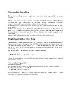
Fig. 1: Base flow separation by Models 1 and 2
is no B1 thus the first observed value is usually equated to B2. The new series starts with the smoothed value of the second observation.
Streamflow
As the method to be chosen for this study ought to be not only acceptable in the literature but must also allow model parameters to be estimated easily from the observed rainfall and/or streamflow data. Boughton (1988) compared two methods of separation of baseflow of which one of them is similar to that described in Equation 2. Both models allow user identification of a point on a hydrograph at which the separation of flow components is apparent. The methods of partitioning of streamflow can be performed in both ways using daily streamflow data as well as hourly streamflow data for flood hydrograph studies. These methods use “manual” identification of one or more points that mark the end of surface runoff but differ in assumptions.
Model1 Model2
Days
Fig. 2: Baseflow in large and small runoff events (Y axis is the Daily Discharge (ml)) Dickson et al. (1967) argued that in the small rises of hydrograph the baseflow discharge shows very quick rise and fall in Model 1 was considered unreasonable. Model 2 appeared a better choice for the general purpose of rainfall-runoff modeling.
Model 1 assumes constant rates of baseflow increase with time; that is, the increase in baseflow and the rate of recharge of baseflow depend on time. The overall increase in the rate of baseflow in the streamflow is closely related to the duration of the surface runoff. Model 2 shows that the rate of increase of baseflow depends on the fraction of the surface runoff; that is, the increase in baseflow and the recharge of baseflow depend on runoff volume.
Model 2 is based on the single exponential smoothing method in time series. It is used to partition the stream flow time series by making the rate of increase of the baseflow proportional to the rate of surface runoff9,21. The rate of increase of baseflow in this model depends on the fraction (α) of the surface runoff (Ai). The rate of baseflow at any time step is Bi, and the separated surface runoff at the same time step is considered to be Ai. Model 2 can be stated as:
The main difference between the two models is that Model 1 estimates more surface runoff and less baseflow than Model 2 for the large events; while Model 1 estimates less surface runoff and more baseflow than Model 2 for small runoff events. Further, Model 2 estimates some surface runoff at every rise in the hydrograph while Model 1 treats many small rises as increases in baseflow as shown in Figure 2.
Bi = Bi −1 + α Ai
(3)
where Ai = TSi − Bi −1 ; TSi is the stream flow at the same time step of Ai. Another way of writing Equation 3 is
Bi = Bi −1 + α (TS i − Bi −1 ) =
αTS i + (1 − α ) Bi −1
1771
(4)
separately to observe the effects of α on baseflow separation.
In this research 50 years of rainfall and streamflow data were used and a separate computer program was written (Fortran) which fits well with the Boughton21 separation process (Model 2). A simpler and practical Boughton’s21 method was examined in this study.
Figure 3 indicates that a value of α = 0.004 provides a more acceptable baseflow separation fit for Event 1; the straight line part of both curves are matched together from the point of recession starts (In the case of α = 0.005 and α = 0.008 the streamflow and baseflow separation lines merged before point of recession curve starts and for α = 0.003 both the streamflow and baseflow separation lines merged after the point of recession curve starts).
While the form is similar to the single exponential smoothing the base flow observed data is not available; excepting the initial value and final point (point of inflection approximated from graphs of daily discharge). The equation is similar to Robert (1959), who used the observation at time t for this value rather than at time t-1 in Equation 3. Usually, the state of control of the process at any time (t,) depends solely on the most recent measurement from the process but in the EWMA technique used, the decision depends on the EWMA statistic; an exponentially weighted average of all prior values. By the choice of weighting factor ( α ), the EWMA control procedure can be made sensitive to a small or gradual drift in the process. 3.
2 1 LogQ
0 -1
0
50
100
150
100
150
100
150
-2 -3 -4 Tim e step
METHOD 2
The study is based on hourly streamflow and rainfall data. Two rural catchments Bremer River catchment (143110A, catchment area 130 sq km2) and Tenhill Creek catchment (143212A, catchment area 447 sq km2) were selected from Queensland. From each catchment four different rainfall streamflow events were selected to estimate an appropriate α value for each catchment. A FORTRAN program was developed to investigate the impact on CL due to the separation of baseflow using exponential smoothing method from the stream flow analysis (Equation 3). The outputs of the FORTRAN program were used to compute the total streamflow, baseflow and CL values out of the total rainfall volume.
1 LogQ
0 -1
0
50
-2 -3 -4 Tim e step
2 1 LogQ
0 -1
0
50
-2 -3 -4 Tim e step
2
4.
RESULTS
1 LogQ
0
When the streamflow diagram is plotted on a semi-log graph paper, the recession curve (the right section of the graph) of the streamflow diagram becomes a line (rather than a curve) with constant slope (Figure 3). To provide the acceptable baseflow separation from the streamflow the value α should be selected in such manner that the baseflow separation line (upper curve) can join the start of the recession part of the streamflow hydrograph; that is, at the start point of the straight line section of the streamflow diagram. Out of many rainfall streamflow events, one rainfall streamflow event was selected and four different values of α were used in that event
-1
0
50
100
150
-2 -3 -4 Tim e step
Fig. 3: Streamflow components (semi-log graph) for Event 1: when α = 0.003, 0 .004, 0.005, 0.008 (Bremer River) The alpha value selected above for Event 1 (α = 0.004) is used to conduct base flow separation for 3 other events in the same catchment. Figure 4 shows that the value of α = 0.004 provides acceptable base flow separation for the other
1772
Table 1: Sensitivity of CL with different α value
events of the same catchment. This analyses showed that for the Bremer River catchment a value of α = 0.004 can be used for baseflow separation for all other streamflow events.
α 0.003 0.004 0.005 0.008 0.003 0.004 0.005 0.008 0.003 0.004 0.005 0.008
Event No Event 1
2
Log Q
1.5
Event 2
1 0.5 0 -0.5
0
20
40
60
80
Event 3
Time step
3
CL 1.147 1.163 1.176 1.211 0.179 0.217 0.251 0.344 0.915 0.927 0.938 0.967
2
0 -1
0
50
100
-2 -3
Log Q
Time step
2 1.5 1 0.5 0 -0.5 0 -1 -1.5 -2 -2.5 -3 -3.5
1.4 1.2 1 0.8 0.6 0.4 0.2 0
150
Continuing loss
Log Q
1
0
0.002
0.004
0.006
0.008
0.01
Alpha 50
100
150
Fig. 5: CL vs α for Bremer River catchment In the case of Tenhill Creek catchment, a single α did not provide acceptable baseflow separation. α’s of 0.010, 0.003, 0.008 and 0.002 provided acceptable baseflow separation as shown in Figure 5.
Time step
Fig. 4: Acceptable value of α = 0.004 used in events 2, 3 and 4 in the Bremer River catchment. The sensitivity of computed loss values with α was then studied. Table 1 shows that for Event 1 in the Bremer River catchment when α = 0.004, CL = 1.16, if α is increased by 25%, the value of CL is varied by 1.11%, if α is decreased by 25%, the value of CL is varied by 1.38%. Little variation in CL value was observed (even with 100% variation in α). Figure 5 shows that a small error in selection of α does not seem to affect the value of CL significantly.
2
Log Q
1.5 1 0.5 0 0
50 100 Tim e step
150
3 2.5
Log Q
2 1.5 1 0.5 0 0
1773
50
100 Tim e s tep
150
200
3
3
2.5 2 Log Q
LogQ
2 1 0 0
20
40
60
1.5 1 0.5 0 -0.5 0
80
-1
50
100
150
200
-1 Tim e step
-2 Tim e step
Fig. 7: In all 1, 2, 3, and 4 events of Tenhill Creek, the α = 0.005 is used.
3 2.5
Log Q
2
Table 2: Sensitivity of CL with different α value
1.5 1
Event No Event 1
0.5 0 -0.5 0
50
100
150
200
-1 Tim e step
Fig.6: Tenhill Creek catchment: Event 1 (α = 0.010); Event 2 (α = 0.003); Event 3 (α = 0.008); Event 4 (α = 0.002)
Event 2
The median (0.0055) was then explored for separation. Figure 6 shows the median value provides a reasonable baseflow separation for the Tenhill Creek catchment using the inflection matching technique described earlier.
Event 3
Event 4 2
Log Q
1.5
CL 1.689 1.714 1.736 1.771 1.475 1.541 1.593 1.671 2.063 2.075 2.087 2.111 0.17 0.224 0.27 0.346
1
As before, α was varied to examine the sensitivity of computed CL values. Table 2 shows that for Event 1 (Tenhill Creek), when α is 0.0055 CL is 1.71, and if α is increased by 20%, the value of CL is varied by 2.78%; if α is decreased by 20%, the value of CL is varied by 1.46%. Thus a 60% variation in the value of α resulted in only 4.8% variation in CL. For the Events 2 and 3, the variation in α value by about 60% causes about 13% and 2% variation in CL value. Figure 8 confirm shows that a small error in selecting α does not affect the value of CL significantly.
0.5 0 0
50 100 Tim e step
150
3 2 LogQ
α 0.004 0.005 0.006 0.008 0.004 0.005 0.006 0.008 0.004 0.005 0.006 0.008 0.004 0.005 0.006 0.008
1 0 0
20
40
60
80
-1 -2 Tim e ste p
3
Continuing lossa
2.5
Log Q
2 1.5 1 0.5 0 0
50
100 Tim e s te p
150
2.5 2 1.5 1 0.5 0 0
200
0.002
0.004
0.006
0.008
Alpha
Fig. 8: CL vs α for Tenhill Creek catchment
1774
0.01
Figure 8 shows that small variation in alpha values did not seem to make a significant difference in the estimated CL values for the Tenhill Creek catchment. 5.
SUMMARY AND CONCLUSION
The exponential smoothing based method of baseflow separation was used to examine the impact of continuing loss for medium sized Queensland rural catchments. It was noted that an acceptable baseflow separation coefficient (α) can be selected for a catchment using a (Fortran) trial 6. ACKNOWLEDGEMENTS The authors wish to thank Brisbane Water (Brisbane City Council - S. Hoverman) and the director of the Centre for Environment Systems Research (Prof R Braddock) and Griffith University. 7. REFERENCES Bethalmy, 1974, Smoothing methods in statistics. Springer-Verlag, New York. Or Nist/Ematech., 2007. e-Handbook of Statistical Methods, Engineering statistics hand book. U.S.A. Boughton, W. C., 1987. Hydrograph analysis as a basis of water balance modelling. The Institution of Engineers, Australia, Civil Engineering Transaction, CE29(1): 8 -33. Boughton, W.C., 1988. Partitioning streamflow by computer. The Institution of Engineers, Australia, Civil Engineering Transaction, pp: 285 -291. Chapman, T.G. and Maxwell, A.I., 1996. Baseflow separation – comparison of numerical methods with tracer experiments, Hydrology and Water Resources Symposium, Institution of Engineers, Australia, Hobart, pp: 539 – 545. Dickinson, W. T., Holland, M. E. and Smith, G.L., 1967. An experimental rainfall –runoff facility. Hydrology paper no. 25, Colorado State University, pp:78. Eckhardt K, 2005. How to construct recursive digital filters for baseflow separation. Hydrological Processes 19, 507-515.
based method together with CL sensitivity analysis. Such a process only requires a small number of stream flow events (3 to 4 streamflow events) thus incurring minimal data, computation and practical costs. It was found that continuing loss was not sensitive to small changes in α. A large (50%) change in α made less than 10% variation in continuing loss suggesting that such a method can be relied upon to make approximations methods can be reliably used. This procedure may be used to estimate input values in design flood estimations. Hill, P.I., Maheepala, U., Mein, R. G., Weinmann, P. E., Empirical analysis of data to derive losses for design flood e+-stimation in South-Eastern Australia. CRC for Catchment Hydrology, Report 96/5, 1996. Hill, P.I., 1993. Extreme flood estimation for the Onkaparinga River catchment. M. Eng., Science Thesis, Department of Civil and Environmental Engineering. University of Adelaide, 1993. Hiscock, K., 2005. Hydrology principles and practice, Blackwell Publishing, Oxford, UK. Hino, M. and Hasebe, M., 1985. Separation of a storm hydrograph into runoff components by both filter separation AR method and environmental isotope tracers. Journal of Hydrology, 85: 251 – 264. Hughes. D. and Hannart. P., 2003 A desktop model used to provide an initial estimate of the ecological instream flow requirements of rivers in South Africa. J. Hydrol. (In press). Institution of Engineers, Australia., 1998. Australian Rainfall and Runoff. Institution of Engineers, Australia, 1987 and 1998. Jackman, A. J. and Hornberger, G.M., 1993. How much complexity is warranted in a rainfall-runoff model? Water Resources Research, 29: 26372649. Kobayashi, D., 1985. Separation of the snowmelt hydrograph by stream temperatures. Journal of Hydrology, 76: 155- 162. Kobayashi, D., 1986. Separation of a snowmelt hydrograph by stream conductance. Journal of Hydrology, 84: 157- 164.
Hall, A.J., 1971. Baseflow recessions and the baseflow hydrograph separation problem. Hydrology papers 1971, The Institution of Engineers, Australia, pp: 159 – 170.
1775
Lyne, V. D. and Hollick, M., 1979. Stochastic time-variable rainfall-runoff modelling, Institution of Engineers, Australia, Hydrology and Water Resources Symposium, Perth, pp: 89 – 92.
Lyne, V. D. and Hollick, M., 1979. Stochastic time-variable rainfall-runoff modelling, Institution of Engineers, Australia, Canberra, pp: 89 – 93. Nathan, R. J. and McMahon, T.A., 1990. Evaluation of automated techniques for baseflow National Symposium of Forest Hydrology, Melbourne, Institution of Engineers, Australia. Nat. Conf. Pub. No. 82/6, pp: 132 – 138. Pilgrim, D., Huff, D. and Steels, T., 1979. Use of specific conductance and contact time relations for separating flow components in storm runoff. Water Resources Research, 15(2): 329 – 339. Roberts, 1959. In Nist/Ematech., 2007. eHandbook of Statistical Methods, Engineering statistics hand book. U.S.A. Shirmohammadi, A., Knisel, W. G. and Sheridan, J.M., 1984. An approximate method of partitioning daily streamflow data. Journal of Hydrology, 74: 335 – 354. Smakhtin VY, 2001. Low flow hydrology: a review. Journal of Hydrology 240:147-186. Snorasson, A., Finnsdottir, H.P., Moss, M., 2002. The extremes of the extremes: extraordinary floods, IAHS publication no 271, UK, 2002.
1776
and recession analysis, Water Resources Research, 26(7): 1465 – 1473. O’Loughlin, E.M., Cheney, N.P., Burns, J., 1982. The bushranger experiment: Hydrological response of a eucalypt catchment to fire. The Firs