forecasting using simple exponential smoothing method
Recommend Documents
forecast the monthly revenue (in crore) using best modelâadditive HoltâWinters exponential smoothing up to January 2021. Keywords: Forecast, levels ...
Simple Holt-Winters, the Additive Holt-Winters, namely the Autoregressive Integrated Moving. Average model. ..... D. Holt âWinters Multiplicative Exponential Smoothing Technique (MHWEM) ..... 51-64. 11.Johnston, Jack and Dinardo, John.
Simple Holt-Winters, the Additive Holt-Winters, namely the Autoregressive ... of the U.S. Dollar against German Mark, found that all structural exchange rate ...
Exponential smoothing schemes weight past observations using exponentially ...
equal to 1/N. In exponential smoothing, however, there are one or more ...
Exponential Smoothing for Forecasting and. Bayesian Validation of Computer
Models. A Thesis. Presented to. The Academic Faculty by. Shuchun Wang.
Oct 27, 2016 - We provide a robust alternative for the exponential smoothing forecaster of Hyndman and Khandakar (2008). For each method of a class of ...
Applications of exponential smoothing to forecasting time series usually rely on three basic methods: simple exponential smoothing, trend corrected exponential ...
Feb 22, 2010 - Department of Econometrics and Business Statistics ... tourist arrivals to Australia and New Zealand ..... of Statistical Software 26, 1â22.
Volatility Forecasting with. Smooth Transition Exponential Smoothing. James W.
Taylor. International Journal of Forecasting, 2004, Vol. 20, pp. 273-286. James ...
Apr 4, 1997 - Despite its popularity, little or no theory exists for exponential smoothing. .... that the asymptotic theory of smoothing factor selection is important.
of the Winter's exponential smoothing and autoregressive moving average models. Both of these models are used to predict the availability of rice stock at ...
Abstract: As many systems depend on electronics, concern for fault tolerance is growing rapidly. For example, a ... Keywords: Double exponential smoothing method, drive-by-wire system, fault tolerant system, predictive .... fault location, and fault
... of the apps below to open or edit this item. pdf-1881\forecasting-with-exponential-smoothing-the-state-space-approac
May 2, 2018 - exponential smoothing model, overnight stays, Serbia. JEL: Q11. Introduction. The impact of seasonal demand variation is one of the dominant ...
business students in introductory courses in operations, management science, ... It is easy to understand and use and most commercial forecasting software ...
Download Best Book Forecasting with Exponential Smoothing: The State Space Approach (Springer Series in Statistics), Dow
Double exponential smoothing computes a trend equation through the data using
a special weighting function that places the greatest emphasis on the most ...
Exponential Smoothing. Prepared for the. MIT System Dynamics in Education
Project. Under the Supervision of. Prof. Jay W. Forrester by. Kevin M. Stange.
double exponential smoothing (DES), holt's (brown) and ... 1 Malaysia National Population and Family Development Board, Ministry of Women, Family and ...
Aug 28, 2015 - Abstract. Exponential smoothing has been one of the most popular forecasting methods for business and industry. Its simplicity and ...
Modeling a musical structure or performance is a coveted research area in scientific analysis of ... smoothing that is commonly used nowadays (Brown 1963).
Sulandari et.al (Forecasting Electricity Demand Using Hybrid Exponential Smoothing-Artificial Neural Network Model). (DSHW), corrects for residual using a ...
MSE = 3215248, MPE = 0.18, and MAPE = 5.41. The best model to forecast the number of domestic departures is the method of Winter's exponential smoothing ...
Jul 30, 2014 - Abstract Simple exponential smoothing (SES) methods are the most ..... using Eq. 5. Step 8 Switch back to the SES method and set l0 = l1 if.
forecasting using simple exponential smoothing method
Aug 24, 2013 - In the paper a relatively simple yet powerful and versatile technique for forecasting time series data â simple exponential smoothing.
FORECASTING USING SIMPLE EXPONENTIAL SMOOTHING METHOD
∗ Department
´ ∗ , Oskar OSTERTAG∗∗ Eva OSTERTAGOVA
of Mathematics and Theoretical Informatics, Faculty of Electrical Engineering and Informatics, Technical University of Koˇsice, Nˇemcovej 32, 042 00 Koˇsice, Slovak Republic, tel.: +421 55 602 2447, e-mail: [email protected] ∗∗ Department of Applied Mechanics and Mechatronics, Faculty of Mechanical Engineering, Technical University of Koˇsice, Letn´a 9, 042 00 Koˇsice, Slovak Republic, tel.: +421 55 602 2460, e-mail: [email protected]
ABSTRACT In the paper a relatively simple yet powerful and versatile technique for forecasting time series data – simple exponential smoothing is described. The simple exponential smoothing (SES) is a short-range forecasting method that assumes a reasonably stable mean in the data with no trend (consistent growth or decline). It is one of the most popular forecasting methods that uses weighted moving average of past data as the basis for a forecast. The procedure gives heaviest weight to more recent observations and smaller weight to observations in the more distant past. The accuracy of the SES method strongly depends on the optimal value of the smoothing constant α. To determine the optimal α value in the paper was used a traditional optimalization method based on the lowest mean absolute error (MAE), mean absolute percentage error (MAPE) and root mean square error (RMSE).
Keywords: time series, simple exponential smoothing model, forecast, smoothing constant, root mean square error
1. INTRODUCTION A time series is a sequence of observations indexed by time, usually ordered in equally spaced intervals and correlated. In our days it is well known the importance of time series studies. These studies provide indicators about a country economy, the unemployment rate, the export and import product rates, etc. The most interesting and ambitious task in time series analysis is to forecast future values. Models are commonly fitted in order to predict future values of a time series [4]. Exponential smoothing methods are the most widely used forecasting methods. The formulation of exponential smoothing forecasting methods arose in the 1950s from the original work of Brown (1959, [2]) and Holt (1957, [6]) who were working on creating forecasting models for inventory control systems. Exponential smoothing is an intuitive forecasting method that weights the observed time series unequally. Recent observations are weighted more heavily than remote observations. The unequal weighting is accomplished by using one or more smoothing parameters, which determine how much weight is given to each observation [9]. The simplest technique of this type, simple exponential smoothing (SES), is appropriate for a series that moves randomly above and below a constant mean (stationary series). It has no trend and no seasonal patterns [16]. The Holt-Winters method, also referred to as double exponential smoothing, is an extension of exponential smoothing designed for trended and seasonal time series. Holt-Winters smoothing is a widely used tool for forecasting business data that contain seasonality, changing trends and seasonal correlation [5]. Exponential smoothing model is a widely used method in time series analysis. This popularity can be attributed to its simplicity, its computational efficiency, the ease of adjusting its responsiveness to changes in the process being forecast, and its reasonable accuracy [11]. Generally, exponential smoothing is regarded as an inexpensive technique that gives good forecast in a wide vac 2012 FEI TUKE ISSN 1335-8243 (print) www.aei.tuke.sk
riety of applications. In addition, data storage and computing requirements are minimal, which makes exponential smoothing suitable for real-time application. 2. SIMPLE EXPONENTIAL SMOOTHING MODEL The simple exponential smoothing (SES) model is usually based on the premise that the level of time series should fluctuate about a constant level or change slowly over the time [9]. 2.1. Mathematical Formulation The SES model is given by the model equation y(t) = β (t) + ε(t),
(1)
where β (t) takes a constant at the time t and may change slowly over the time; ε(t) is a random variable and is used to describe the effect of stochastic fluctuation. Let an observed time series be y1 , y2 , . . . , yn . In any case, in this simple model, to predict yt is merely to predict (estimate) β . To estimate, it makes sense to use all the past observations, but due to declining correlation as you go back into the past, to down-weight older observations. Formally, the simple exponential smoothing equation takes the form of Ft+1 = α yt + (1 − α)Ft ,
(2)
where yt is the actual, known series value at the time t; Ft is the forecast value of the variable Y at the time t; Ft+1 is the forecast value at the time t + 1; α is the smoothing constant [3]. The forecast Ft+1 is based on weighting the most recent observation yt with a weight α and weighting the most recent forecast Ft with a weight of 1 − α. To get started the algorithm, we need an initial forecast, an actual value and a smoothing constant. Since F1 is not known, we can: • Set the first estimate equal to the first observation. Further we will use F1 = y1 .
Unauthenticated | 88.212.40.94 Download Date | 8/24/13 5:56 AM
ISSN 1338-3957 (online) www.versita.com/aei
Acta Electrotechnica et Informatica, Vol. 12, No. 3, 2012
63
• Use the average value of the first few observations of the data series for the initial smoothed value.
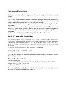
Weights on different lags 0.7 weight 0.2 weight 0.5 weight 0.7 0.6
Smoothing constant α is a selected number between zero and one, 0 < α < 1. Rewriting the model (2) we can see one of the neat things about the SES model (3)
change in forecasting value is proportional to the forecast error. That is
where Ft+1 is the forecast value of the variable Y at the time t + 1 from knowledge of the actual series values yt , yt−1 , yt−2 and so on back in time to the first known value of the time series, y1 [3, 13]. Therefore, Ft+1 is the weighted moving average of all past observations. The series of weights used in producing the forecast Ft+1 is α, α(1 − α), α(1 − α)2 , . . .
(7)
It is obviously from (7) that the weights are exponential; hence the name exponentially weighted moving average [1]. The exponential decline of the weights toward zero is evident. This is shown in Figure 1. The decay is slower for small values α, so we can control the rate of decay by choosing α appropriately. c 2012 FEI TUKE ISSN 1335-8243 (print) www.aei.tuke.sk
6
8
10 Time
12
14
16
18
20
2.2. Measuring Forecast Error After the model specified, its performance characteristics should be verified or validated by comparison of its forecast with historical data for the process it was designed to forecast. This is no consensus among researchers as to which measure is best for determining the most appropriate forecasting method. Accuracy is the criterion that determines the best forecasting method; thus, accuracy is the most important concern in evaluating the quality of a forecast. The goal of the forecast is to minimize error [14]. Some of the common indicators used to evaluate accuracy are MAE (Mean absolute error), MSE (Mean squared error), RMSE (Root mean squared error) or MAPE (Mean absolute percentage error): MAE =
1 n ∑ |et |, n t=1
(8)
MSE =
1 n 2 ∑ et , n t=1
(9)
RMSE =
√ MSE
(10)
MAPE =
1 n |et | ∑ yt · 100 %, n t=1
(11)
(6)
k=0
4
Fig. 1 Exponentially declining weights
t−1
Ft+1 = α
2
(5)
is the forecast error at the time t. So, the exponential smoothing forecast is the old forecast plus an adjustment for the error that occurred in the last forecast [1, 12]. By iterating formula (2) we get: F1 = y1 ;
0
where yt is the actual value at the time t; et is residual at the time t; n is the total number of the time periods. MAE is a measure of overall accuracy that gives an indication of the degree of spread, where all errors are assigned equal weights. If a method fits the past time series data very good, MAE is near zero, whereas if a method fits the past time series data poorly, MAE is large. Thus, when two or more forecasting methods are compared, the one with the minimum MAE can be selected as most accurate [14]. MSE is also a measure of overall accuracy that gives an indication of the degree of spread, but here large errors
Unauthenticated | 88.212.40.94 Download Date | 8/24/13 5:56 AM
ISSN 1338-3957 (online) www.versita.com/aei
64
Forecasting Using Simple Exponential Smoothing Method
are given additional weight. It is a generally accepted technique for evaluating exponential smoothing and other methods [7]. Often the square root of MSE, RMSE, is considered, since the seriousness of the forecast error is then denoted in the same dimensions as the actual and forecast values themselves. MAPE is a relative measure that corresponds to MAE. It is the most useful measure to compare the accuracy of forecasts between different items or products since it measures relative performance. It is one measure of accuracy commonly used in quantitative methods of forecasting [10]. If MAPE calculated value is less than 10 %, it is interpreted as excellent accurate forecasting, between 10–20 % good forecasting, between 20–50 % acceptable forecasting and over 50 % inaccurate forecasting [8]. Selection of an error measure has an important effect on the conclusions about which of a set of forecasting methods is most accurate.
Table 1 Observed values of primary production of electricity
The accuracy of forecasting of SES technique depends on smoothing constant. Choosing an appropriate value of exponential smoothing constant is very crucial to minimize the error in forecasting. Selecting a smoothing constant is basically a matter of judgment or trial and error, using forecast errors to guide the decision. The goal is to select a smoothing constant that balances the benefits of smoothing random variations with the benefits of responding to real changes if and when they occur. The smoothing constant serves as the weighting factor. When α is close to 1, the new forecast will include a substantial adjustment for any error that occurred in the preceding forecast. When α is close to 0, the new forecast is very similar to the old forecast. The smoothing constant α is not an arbitrary choice but generally falls between 0.1 and 0.5. Low values of α are used when the underlying average tends to be stable; higher values are used when the underlying average is susceptible to change. In practice, the smoothing constant is often chosen by a grid search of the parameter space; that is, different solutions for α are tried starting, for example, with α = 0.1 to α = 0.9, with increments of 0.1 [1,12]. The value of α with the smallest MAE, MSE, RMSE or MAPE is chosen for use in producing the future forecasts. 3. EXAMPLE FROM TECHNICAL PRACTICE The simple exponential smoothing model can be illustrated by using data about primary production of electricity (yt ) in terajoules (TJ) in Slovakia over the years 2001–2009 that are in the Table 1 [17]. We want to forecast primary production of electricity in Slovakia for the year 2010. We can see from the plot that there is roughly constant level. Thus, we can make forecasts using SES method. It is illustrated in Figure 2. c 2012 FEI TUKE ISSN 1335-8243 (print) www.aei.tuke.sk
Production of electricity [TJ]
1.8
2.3. Choosing the Best Value for Smoothing Constant
1.7
1.6
1.5
1.4
1.3
1.2
1
2
3
4
5 Time period
6
7
8
9
Fig. 2 Observed time series data
In this study were adopted to assess the accuracy of forecasting methods three accuracy models – MAE, MAPE and RMSE. These error measures were calculated using equations (2), (5) and (8)–(11) for different values of exponential smoothing constant using MATLAB. Table 2 shows the values of MAE, MAPE and RMSE for different α. Table 2 MAE, MAPE, RMSE for different values of α
α 0.25 0.26 0.27 0.28 0.29 0.30
MAE 1405.09 1402.04 1399.27 1396.76 1394.53 1396.23
Values of MAE, MAPE, and RMSE depend on the choice of the smoothing constant. MAE and MAPE are decreased with increasing α up to 0.29 and after that MAE and MAPE are increased. Variation of MAE with α is shown in Figure 3 and variation of MAPE with α is shown in Figure 4.
Unauthenticated | 88.212.40.94 Download Date | 8/24/13 5:56 AM
ISSN 1338-3957 (online) www.versita.com/aei
Acta Electrotechnica et Informatica, Vol. 12, No. 3, 2012
65
1900 1850 1800 1750
MAE
1700 1650 1600 1550 1500 1450 1400 1350 0.1
0.2
0.3
0.4
0.5 0.6 Smoothing constant α
0.7
0.8
0.9
Fig. 3 Variation of MAE for different values of α
RMSE is decreased with increasing α up to 0.26 and after that RMSE is increased. Variation of RMSE with α is shown in Figure 5. To find the optimal value of smoothing constant, minimum values of MAE, RMSE and MAPE are selected and corresponding value of smoothing constant is the optimal value for this problem [13]. By calculating the forecast values using equation (1) for α = 0.29 and α = 0.26, we obtain the values presented in the columns 3–4 in the Table 3. In the last line in the Table 3 are forecast results for the time period 10, therefore for year 2010. So the forecast of primary production of electricity in Slovakia for year 2010 by using α = 0.29 is about 15660 TJ and by using α = 0.26 it is about 15717 TJ. For both values of alpha was obtained result value of MAPE less than 10 % and it means the excellent accurate forecasting. Table 3 Forecast values for minimum MAE, MAPE and RMSE
13
Period t 1 2 3 4 5 6 7 8 9 10
12.5
12
MAPE
11.5
11
10.5
10
9.5 0.1
0.2
0.3
0.4
0.5 0.6 Smoothing constant α
0.7
0.8
0.9
Fig. 4 Variation of MAPE for different values of α
This concept is illustrated in Figure 6 which shows a time series observed for periods 1 to 9 and corresponding forecast values for period 10 by using α = 0.29 and α = 0.26.
Fig. 5 Variation of RMSE for different values of α Fig. 6 Comparison of observed values and forecast values using α = 0.29 and α = 0.26 c 2012 FEI TUKE ISSN 1335-8243 (print) www.aei.tuke.sk
Unauthenticated | 88.212.40.94 Download Date | 8/24/13 5:56 AM
ISSN 1338-3957 (online) www.versita.com/aei
66
Forecasting Using Simple Exponential Smoothing Method
4. RESULTS The purpose of this paper was to evaluate forecast accuracy by using data of primary production of electricity in Slovakia. It is therefore aimed to analyse SES forecasting method. To estimate optimal value of smoothing constant, forecasts are computed with α = 0.1 to α = 0.9, with increments of 0.01. Three forecasting accuracy techniques, such as MAE, MAPE, and RMSE are used to select the most accurate forecast for one year ahead forecast. 5. DISCUSSION/CONCLUSIONS The exponential smoothing provides an idea that the most recent observations usually give the best guide to the future, therefore we want a weighting scheme with decreasing weights for older observations. The choice of the smoothing constant is important in determining the operating characteristics of exponential smoothing. The smaller the value of α, the slower the response. Larger values of α cause the smoothed value to react quickly – not only to real changes but also random fluctuations [11]. Simple exponential smoothing model is only good for non-seasonal patterns with approximately zero trend and for short-term forecasting because if we extend past the next period, the forecasted value for that period has to be used as a surrogate for the actual demand for any forecast past the next period. Consequently, there is no ability to add corrective information (the actual demand) and any error grows exponentially. ACKNOWLEDGEMENT This article was created by implementation of the grant project VEGA No. 1/0102/11 Experimental methods and modeling techniques in-house manufacturing and non manufacturing processes.
[9] LI, Z. P. – YU, H. – LIU, Y. C. – LIU, F. Q.: An Improved Adaptive Exponential Smoothing Model for Short Term Travel Time Forecasting of Urban Arterial Street, Acta automatica sinica, Vol. 34, No. 11, 1404– 1409, 2008. [10] MAKRIDAKIS, S. – WHEELWRIGHT, S. C. – HYNDMAN, R. J.: Forecasting Methods and Applications, New York, Wiley, 1998. [11] MONTGOMERY, D. C. – JOHNSON, L. A. – GARDINER, J. S.: Forecasting and Time Series Analysis, McGraw-Hill, Inc., 1990, ISBN 0-07-042858-1. ´ E.: Applied Statistics, [in Slovak], [12] OSTERTAGOVA, Elfa, Koˇsice, 2011, ISBN 978-80-8086-171-1. ´ E. – OSTERTAG, O.: The Simple [13] OSTERTAGOVA, Exponential Smoothing Model, Proceedings of the 4th International Conference on Modelling of Mechanical and Mechatronic Systems, Technical University of Koˇsice, Slovak Republic, 380–384, 2011. [14] RYU, K. – SANCHEZ, A.: The Evaluation of Forecasting Methods at an Institutional Foodservice Dining Facility, The Journal of Hospitality Financial Management, Vol. 11, No. 1, 2003. [15] SANJOY, K. P.: Determination of Exponential Smoothing Constant to Minimize Mean Square Error and Mean Absolute Deviation, Global journal of research in engineering, Vol. 11, 2011. [16] YORUCU, V.: The Analysis of Forecasting Performance by Using Time Series Data for Two Mediterranean Island, Review of Social, Economic & Business Studies, Vol. 2, 175–196, 2003. [17] http://www.statistics.sk. Received June 14, 2012, accepted September 24, 2012
REFERENCES [1] ACZEL, A. D.: Complete Business Statistics, Irwin, 1989, ISBN 0-256-05710-8. [2] BROWN, R. G.: Statistical Forecasting for Inventory Control, McGraw-Hill: New York, 1959. [3] BROWN, R. G. – MEYER, R. F.: The Fundamental Theory of Exponential Smoothing, Operations Research, 9, 673–685, 1961. [4] CORDEIRO, C. – NEVES, M. M.: Bootstrap and Exponential Smoothing Working together in Forecasting Time Series, Proceedings in Computational Statistics, Physica-Verlag, 891–899, 2008. [5] GELPER, S. – FRIED, R. – CROUX, CH.: Robust Forecasting with Exponential and Holt Winters Smoothing, Journal of forecasting, Vol. 29, No. 3, 285–300, 2010. [6] HOLT, C. C.: Forecasting trends and seasonals by exponentially weighted averages, O.N.R. Memorandum 52/1957, Carnegie Institute of Technology, 1957. [7] JARETT, J.: Business Forecasting Methods, Cambridge, MA: Basil Blackwell, 1991. c 2012 FEI TUKE ISSN 1335-8243 (print) www.aei.tuke.sk
[8] LEWIS, C. D.: Industrial and Business Forecasting Methods, London, Butterworths, 1982.
BIOGRAPHIES Eva Ostertagov´a (PhDr, PhD) graduated (MSc) at the ˇ arik University Faculty of Natural Sciences at the P. J. Saf´ in Koˇsice. She defended her PhD at the Faculty of Mechanical Engineering at Technical University in Koˇsice. She is working as an assistant professor the applied mathematics at the Faculty of Electrical Engineering and Informatics, Technical University in Koˇsice. Her scientific research is application of the mathematical modelling in automation and control in industry. Oskar Ostertag (Doc, Ing, PhD) graduated (MSc) at the Faculty of Mechanical Engineering at Technical University in Koˇsice. He defended his PhD at the Faculty of Mechanical Engineering at Technical University in Koˇsice. He is working as an associated professor of the applied mechanics at the Faculty of Mechanical Engineering at Technical University in Koˇsice. His scientific research is application of the analytical and numerical methods in construction parts designing.
Unauthenticated | 88.212.40.94 Download Date | 8/24/13 5:56 AM