Based Particle Swarm Optimization for a ... - Wiley Online Library

Computer-Aided Civil and Infrastructure Engineering 29 (2014) 771–800

Antithetic Method-Based Particle Swarm Optimization for a Queuing Network Problem with Fuzzy Data in Concrete Transportation Systems Ziqiang Zeng Uncertainty Decision-Making Laboratory, Sichuan University, Chengdu 610064, P.R. China

Jiuping Xu* State Key Laboratory of Hydraulics and Mountain River Engineering, Sichuan University, Chengdu 610065, P.R. China and Uncertainty Decision-Making Laboratory, Sichuan University, Chengdu 610064, P.R. China

Shiyong Wu & Manbin Shen Ertan Hydropower Development Company, Ltd., Chengdu, P.R. China

Abstract: The aim of this article is to develop an antithetic method-based particle swarm optimization to solve a queuing network problem with fuzzy data for concrete transportation systems. The concrete transportation system at the Jinping-I Hydropower Project is considered the prototype and is extended to a generalized queuing network problem. The decision maker needs to allocate a limited number of vehicles and unloading equipment in multiple stages to the different queuing network transportation paths to improve construction efficiency by minimizing both the total operational costs and the construction duration. A multiple objective decisionmaking model is established which takes into account the constraints and the fuzzy data. To deal with the fuzzy variables in the model, a fuzzy expected value operator, which uses an optimistic–pessimistic index, is introduced to reflect the decision maker’s attitude. The particular nature of this model requires the development of an antithetic method-based particle swarm optimization algorithm. Instead of using a traditional updating method, an antithetic particle-updating mechanism is designed to automatically control the particleupdating in the feasible solution space. Results and a sensitivity analysis for the Jinping-I Hydropower Project are presented to demonstrate the performance of our optimization method, which was proved to be very effective ∗ To whom correspondence should be addressed. E-mail: xujiuping@ scu.edu.cn.

 C 2014 Computer-Aided Civil and Infrastructure Engineering. DOI: 10.1111/mice.12111

and efficient compared to the actual data from the project and other metaheuristic algorithms. 1 INTRODUCTION New and renewable sources of energy, such as hydropower resources, have become more important in the world today. Hydropower resources, one of the more popular renewable energy sources, play an important role in China, especially in Sichuan Province. The Chinese government has emphasized renewable energy development, particularly in the areas of water conservancy and hydropower. The Ertan Hydropower Development Company, Ltd. (EHDC) was appointed to supply clean and renewable energy to support the economic and social development of the Sichuan–Chongqing region through the development of hydropower resources on the Yalong River in Sichuan. The Jinping-I Hydropower Project, which is presently under construction, is one of EHDC’s projects. This article focuses on vehicle and unloading equipment scheduling to achieve queuing network optimization for the concrete transportation systems at the Jinping-I Hydropower Project, with the aim of minimizing both total operational costs and construction duration. Queuing decision problems are often encountered in many practical systems, such as flexible manufacturing systems (FMS) (Vakharia et al., 1999), telecommunication systems (Il Choi et al., 2007), field

772

Zeng, Xu, Wu & Shen

service support systems (Papadopoulos, 1996), transportation systems (Jiang and Adeli, 2004; Kim, 2009; Karim and Adeli, 2003; Ghosh-Dastidar and Adeli, 2006; Bliemer, 2007; Szeto et al., 2011; Putha et al., 2012; Balsamo et al., 2003), and flow-shop-type production systems (Kumar and Singh, 2007). Queuing decision models play an important role in queuing system designs, and typically involve making one or a combination of decisions, such as deciding on the number of servers at a service facility, the efficiency of the servers, and the number of service facilities required (Chen, 2007). There has been significant research on queuing networks which include the development of methodologies, theoretical studies, and practical applications (Daduna and Szekli, 2002; Kogan, 2002; Abramov, 2001; Gerasimov, 2000; Casale, 2011; George and Xia, 2011; Harrison and Coury, 2002). Although these studies have significantly improved queuing decision theory and applications, they are as yet incapable of reflecting the queuing features of construction systems. In fact, the construction system queuing network is quite different from those mentioned above (Govil and Fu, 1999; Van and Vandaele, 2007). In the Jinping-I Hydropower Project concrete transportation system, the vehicles transport concrete in a queuing network, which is a multistage network optimization system under uncertainty (Garvin and Cheah, 2004; Kim et al., 2008). To improve construction efficiency, the decision maker needs to determine an optimal allocation schedule for these vehicles using different transportation paths (i.e., multiclass) between the construction mix buildings and the queuing network unloading sites, and also needs to assign in multiple stages an appropriate number of unloading equipment to the unloading sites to guarantee the working efficiency at each queuing location to minimize the total operational costs and the construction duration. This leads to a queuing network problem (QNP). Some uncertain information in the QNP, however, has rarely been considered in the literature. When this problem is considered using deterministic estimated data, there is a deviation between the actual value and the estimated deterministic value of these data. This may lead to misleading decision making, which may result in an inaccurate estimation of the number of vehicles and unloading equipment needed and consequently result in higher total operational costs or longer construction durations. In some situations, random theory has been applied to deal with this uncertain queuing problem data. For example, the servicing and arrival rates have been usually considered stochastic distributions (De Vuyst et al., 2002; Ivnitski, 2001). Although it is well known that random modeling techniques are useful tools in dealing with queuing problem uncertainty, in the real world, there are many nonprobabilistic factors that affect large-scale

hydropower construction projects, and therefore, fuzzy theory is more suitable. When comparing the essence of these two uncertain approaches, it can be seen that they are quite different in applicability. The fuzzy approach is suitable for subjective uncertainty, which is useful when different engineers have different conclusions about the same thing. Thus, fuzzy set theory has the characteristics of gradualness, uncertainty, vagueness, and bipolarity (Dubois and Prade, 2012). On the other hand, the random approach is useful for situations in which there is objective uncertainty, and is generally calculated using historical data and analyzed using statistical methods. In a hydropower construction project, however, because each project generally has a unique construction technology, differing geographical situations and crew formations, and other specific conditions, at the beginning, as there is no historical project data, it is difficult to determine random variables accurately by using historical data from other projects. In this study, the collected data are established in close consultation with site engineers, but different engineers have different conclusions about the data. However, as the collected data, which are described in linguistic terms by the different experienced engineers through interviews, are usually within a certain range, there is a value that represents the mean of all the observed data. For this reason, the fuzzy method is an effective approach. First proposed by Zadeh (1965), and consequently developed by researchers such as Dubois and Prade (1988), and Nahmias (1978), fuzzy theory has been a useful tool in dealing with ambiguous information in many fields, such as machine learning (Adeli and Hung, 1995), computer science (Jiang and Adeli, 2003; Yan and Ma, ` 2012a, b, 2013; Fougeres and Ostrosi, 2013; Liu and Er, 2012; Theodoridis et al., 2012; Subramanian and Suresh, 2012), and transportation engineering (Adeli and Jiang, 2003). Rahmati and Pasandideh (2012) pointed out that, in a system such as a queuing system, the fuzzy method has a higher validity than random theory to prevent the effect of uncertainty when there is no historical data or only imprecise data, particularly when human behavior can impact the operations. In this article, a QNP under a fuzzy environment is considered, and fuzzy theory is used to deal with the uncertain information when modeling the concrete transportation systems for the Jinping-I Hydropower Project. The QNP is actually a nonlinear integer programming problem. It is well known that linear integer programming is an NP-hard problem (Nemhanser and Wolsey, 1988) and is significantly more difficult than linear integer programming. Although there have been some exact algorithms which have been proven to solve nonlinear integer programming under some specific conditions (Tian and Zhang, 2004; Wang et al., 2011), most are only able to effectively solve simple or

AM-based PSO for queuing networks problem

small-scale problems. However, regardless of the current state-of-the-art of these exact techniques, complex or large-scale nonlinear integer programming problems cannot be solved optimally in a reasonable amount of time, nor have they performed well consistently. As methods based on meta-heuristics need to be designed for each individual problem, it is often difficult to find a usual or normal pattern. Although there have been many competitive meta-heuristic methods such as the genetic algorithm (GA) (Holland, 1992), simulated annealing (SA) (Kirkpatrick et al., 1983), ant colony optimization (ACO) (Mohan and Baskaran, 2012), the particle swarm optimization (PSO) (Kennedy and Eberhart, 1995), which has been adapted widely in such areas as control systems (Bolat et al., 2013), decision sciences (Wang et al., 2009), network optimization (Nyirenda et al., 1978), renewable energy development (Khare and Rangnekar, 2013), and data clustering (Rana et al., 2011), is proposed for the optimization in this article due to its outstanding learning mechanisms, computational tractability, and easy implementation, all of which distinguish it from other meta-heuristic optimization techniques. In this study, an antithetic method-based particle swarm optimization (AM-based PSO) is developed based on an antithetic particleupdating mechanism. This improved algorithm, which is designed based on the particular nature of the model to solve the above optimization problem, is able to automatically control the particle-updating in the feasible solution space and to avoid redundant searching for infeasible particle positions. 2 PROBLEM STATEMENT Concrete transportation is a multiclass queuing network problem, in which a decision maker allocates vehicles to different transportation paths running between concrete mixing buildings and unloading sites in the queuing network, and assigns in multiple stages the appropriate number of unloading equipment to the unloading sites to guarantee working efficiency at each queuing location to minimize total operational costs and construction duration. 2.1 Concrete construction in high arch dam project Most construction projects involve a combination of repetitive and nonrepetitive tasks (Adeli and Karim, 1997). A typical example of repetitive task in a concrete high arch dam construction project is the vehicle transportation of the concrete from the concrete production site to the concrete pouring site. The entire concrete construction process can be divided into three types of systems: concrete production, concrete transportation, and concrete pouring, as shown in Figure 1. In a

773

large-scale hydropower project, there is usually one concrete production system as shown in the dashed box in the lower center of Figure 1. The concrete production system has several concrete mixing buildings (the circles in the dashed box). For example, there are three concrete mixing buildings at the Jinping-I Hydropower Project. In practice, the number of concrete mixing buildings is determined according to the operational cost (i.e., upper limit) and the concrete pouring intensity (i.e., lower limit). Vehicles (the little white rectangles) queue at the concrete mixing buildings to load the concrete, and then, under a heavy-load, transport it to the unloading sites (the dashed triangles) for use in the concrete pouring system (the dashed large rectangle at the top of Figure 1). At the Jinping-I Hydropower Project, there are four parallel routes to the four unloading sites. The cable machines (the little black rectangles) unload the concrete from the vehicles at the unloading site and transport it to the corresponding pouring area (the shaded area in the high arch dam). At the Jinping-I Hydropower Project, a cable machine is able to unload one vehicle at a time and can only serve nominated sections of the dam. When the vehicles arrive at the corresponding unloading site, they queue to unload the concrete into the waiting cable machines (i.e., unloading equipment), and then return to the concrete mixing building for the next load. At the Jinping-I Hydropower Project, the queuing area at the concrete mixing buildings is able to accommodate about 60 waiting vehicles, and the queuing area at each unloading site is able to accommodate about 20 vehicles. The vehicles and the transportation paths between the concrete mixing buildings and the unloading sites in the queuing network form the complete concrete transportation system. 2.2 Queuing networks in a concrete transportation system Usually, one concrete production system is responsible for supplying concrete to several unloading sites, especially in large-scale construction projects. Each unloading site is in charge of its corresponding pouring area and may have several pieces of unloading equipment (i.e., cable machines) between them. The vehicles are divided into several teams and allocated to tasks on different transportation paths connecting the concrete production system with its corresponding unloading sites. Figure 2 shows an example in which N unloading sites share one concrete production system. Because the task of the different vehicle teams is to transport concrete from the concrete production system to the different unloading sites, the vehicles can be regarded as different classes of customers, which means this is a multiclass queuing network problem. The transportation paths in the queuing network meet at an intersection (i.e., the

774

Zeng, Xu, Wu & Shen

Fig. 1. Concrete production, transportation, and pouring systems.

concrete production system) and send different vehicle teams to their corresponding unloading sites and then they return, as shown in Figure 2. 2.3 Multiple stage QNP optimization The entire concrete construction process for a high arch dam can be divided into three stages according to the concrete pouring sequence. These three stages are in order: foundation concrete pouring, central dam concrete pouring, and upper dam concrete pouring, as shown in Figure 3. The types of concrete needed for the different pouring areas are dependent on the pouring stages. The different types of concrete used at each stage mean that there are different service rates at the concrete mixing buildings in the concrete production system. The concrete pouring quantity for each pouring area is also different depending on the construction stage. As shown in Figure 3, each unloading site has an independent transport path connected to the concrete production system. In each stage, all available vehicles are allocated to different transport paths. Further, the equipment failure rate for each type of vehicle (or unloading equipments) may be different on different transport paths (or unloading sites) and in different

stages (Xu and Zeng, 2012). Usually, equipment failure in the vehicles (or unloading equipment) occurs gradually instead of as a sudden breakdown. Thus, when a vehicle (or a piece of unloading equipment) falls into fatigued state during a stage, it is able to keep working until the end of this stage, and is then sent to the maintenance department. Because the vehicle (or unloading equipment) maintenance is a timeconsuming job, all delays due to repair are denoted to be ζ stages. When the repairs are completed, the vehicle (or unloading equipment) is sent back to work in the concrete transportation system. Therefore, the number of available vehicles (or unloading equipment) in a stage decreases due to the equipment failures in the preceding stage and increases as repaired vehicles (or unloading equipment) return to work with the supplemental ones provided in the current stage. Based on the dynamic change in the amount of available vehicles in different stages, decision makers need to make multiple stage decisions to optimize the allocation of all vehicles and unloading equipment at each stage to minimize both the total operational costs and the construction duration. It should be noted that there are no switching costs between stages. All concrete mixing buildings switch from one stage to another simultaneously.

AM-based PSO for queuing networks problem

775

3 MODELLING APPROACH To add to this complexity, effective monthly working days, transportation and stay times, vehicle arrival rate, and the facilities service rate are all considered to be under a fuzzy environment, as explained in the following. To facilitate the model presentation, some of the important notations used hereafter are summarized in Table 1. 3.1 Motivation for employing fuzzy variables

Fig. 2. Concrete transportation system queuing network.

The need to address uncertainty in construction management is widely recognized, as uncertainties exist in a variety of system components. As a result, the inherent complexity and uncertainty existing in real-world queuing decision problems has essentially placed them beyond conventional deterministic optimization methods. Although probability theory has been proved to be a useful tool for dealing with uncertainty in queuing decision problems in manufacturing systems (Govil and Fu, 1999), sometimes it may not be suitable for new construction projects due to the lack of historical data for some important parameters. Although it may be easy to estimate the probability distributions for the production facilities service rate (Papadopoulos and Heavey, 1996) if there is insufficient historical data, it is usually difficult to do this for the construction equipment service rate, the vehicle arrival rates, the effective monthly working days, the transportation and stay times, and the other important parameters in a new construction project, especially in the early construction stages. In this case, fuzzy theory is more suitable to deal with such situations encountered in the QNP. As the collected observed data are based on the engineers’ experience, different engineers may come to different conclusions. The collected data from interviews with the engineers are described in linguistic terms, such as “the range of the value is between r1ϑ and r3ϑ , with the most likely value being r2ϑ ” (i.e., ϑ = 1, 2, . . . , E, where ϑ is the index of engineers). For this reason, in this article, a fuzzy variable is employed to characterize the uncertainty encountered in the QNP. In this way, the decision making under a fuzzy environment is able to adequately measure the human behavioral influences on the project practice. Thus, the optimization results for the QNP under a fuzzy environment are quite useful and may serve as a reference for decision makers in guiding current practice. 3.2 Construction of fuzzy membership functions

Fig. 3. Multistage optimization for queuing decision problems.

In most cases, the methods used for formulating fuzzy membership functions can be classified into three approaches: construction using the analyst’s judgment,

776

Zeng, Xu, Wu & Shen

Table 1 Notations for the model and algorithm parameters and variables Certain Parameters A E (k) and A V (k): number of available unloading equipment, and vehicles for a transportation system in Stage k An kg and Or gk : set of antithetic, original elements in Group g of Part k of a velocity or a particle position Ce , Cb , and Cv : unit operational cost for the unloading equipment at a pouring area (CNY/day), a concrete mixing building in a construction production system (CNY/day), and a vehicle (CNY/day) c p and cg : acceleration coefficients that determine the relative weight that the global best solution has versus the personal best solution D: most endurable construction duration for the transportation system Di (k): concrete construction duration at Pouring Area i in Stage k (month) E Me [γ˜ ]: expected value of γ˜ G Best: global best solution among all the particle swarms achieved so far H : heaped capacity for a vehicle (m3 /vehicle) Iid (k) and Iim (k): pouring intensity at Pouring Area i in Stage k for (m3 /day) and (m3 /month), respectively k k and Polq : normalized probability of antithetic, original elements Palq P Bestl : personal best solution of the lth particle encountered after τ iterations j j pi (k): limit probability of state Si (k) Pl (τ ): position of a particle (i.e., a possible solution), where Pl (τ ) = [ pl1 (τ ), pl2 (τ ), . . . , pl(2N ×3) (τ )] Q i (k): required concrete pouring quantity at Pouring Area i in Stage k (m3 ) r p and r g : random numbers between 0 and 1 j Si (k): state at Unloading Site i in Stage k when there are j vehicles unloading and queuing t: work time of vehicles (hour/day) Vl (τ ): position change for a particle, where Vl (τ ) = [vl1 (τ ), vl2 (τ ), . . . , vl(2N ×3) (τ )] w(τ ): inertia weight used to control the impact of the previous velocities on the current velocity ylqk (τ ): the qth dimension of Ylk (τ ) for the lth particle in the τ th generation, where q = 1, 2, . . . , 2N Ylk (τ ): the kth part of a possible solution in the τ th generation (i.e., the values of decision variables vi (k) and ei (k)) made in Stage k k k k (τ ), zl2 (τ ), . . . , zl(2N Z lk (τ ): the kth part of the lth velocity in the τ th generation, where Z lk (τ ) = [zl1 ) (τ )] k k zlq (τ ): the qth dimension of Z l (τ ) for the lth velocity in the τ th generation, where q = 1, 2, . . . , 2N α1 and β1 : number of available vehicles and unloading equipment allocated to a transportation system in Stage 1 ψi (k) and φi (k): equipment failure rates for the vehicles and unloading equipment allocated to Subsystem i in Stage k RV (k + 1) and R E (k + 1): number of supplemental vehicles and unloading equipment in Stage k + 1 Uncertain Parameters i (k): total time needed for a vehicle transporting between Unloading Site i and the concrete production system in Stage k T c (k) and T ui (k): stay and waiting times in the concrete production system, Unloading Site i in Stage k T i  hi (k): empty-load, heavy-load transportation time on Path i in Stage k Te (k) and T w : effective monthly working days (day/month)  λi (k): arrival rate of a vehicle when arriving at Unloading Site i in Stage k j  λi (k): arrival rate of Unloading Site i in Stage k when there are j vehicles unloading and queuing μ˜ i (k): service rate for the unit unloading equipment at Unloading Site i in Stage k j μ˜ i (k): service rate for Unloading Site i in Stage k when there are j vehicles at Unloading Site i ρ˜i (k): ratio of arrival rate and service rate ξ˜i (k): service rate for Unloading Site i in Stage k (vehicle/hour) Variables ei (k): number of unloading equipment allocated to Unloading Site i in Stage k vi (k): number of vehicles allocated to Subsystem i in Stage k Functions ∼

∼

f c (x, θ ) and f d (x, θ ): objective function for operational cost (CNY) and construction duration (month)

AM-based PSO for queuing networks problem

construction using experiments, or construction using a given numerical data set (Lee et al., 2006; Adeli and Karim, 2000). Selecting a method to determine the membership functions depends on many conditions, including the characteristics of the study and the available data set associated with the study (Lee and Donnell, 2006). Fuzzy set theory deals with a set of objects characterized by a membership (characteristic) function that assigns to each object a grade of membership ranging between zero (no membership) and one (full membership) (Zadeh, 1965). The concept of “unsharp boundaries” that fuzzy set theory represents mimics the human way of thinking, which works in shades of gray rather than black and white. The fuzzy number mathematical operations (i.e., addition, subtraction, multiplication, and division) are processed using the definition given by Dubois and Prade (1978). In this study, the triangular membership function is considered the most appropriate type for characterizing the observed data. Because the triangular membership function can be expressed as a triangular fuzzy number (i.e., γ˜ = [(r1 , r2 , r3 )]), the mean (i.e., r2 ), the left border (i.e., r1 ) and the right border (i.e., r3 ) of the fuzzy number are determined from the engineers’ experience. In order to collect the data, interviews were conducted with differently experienced engineers (i.e., ϑ = 1, 2, . . . , E, where ϑ is the index of engineers). The observed data are described in linguistic terms such as “between 0.28 and 0.40, with the most likely value being 0.34.” The engineers presented the linguistic terms based on their observed data over time. Generally, the view of each engineer can be denoted as a range in the observed data (i.e., [r1ϑ , r3ϑ ]) and a most likely value (i.e., r2ϑ ). Because different engineers have different views regarding the observed data, the minimal value of all r1ϑ and the maximal value of all r3ϑ (for ϑ = 1, 2, . . . , E) are selected as the left border (i.e., r1 ) and the right border (i.e., r3 ) of the triangular fuzzy number γ˜ , respectively. The expected value of all the r2ϑ (for ϑ = 1, 2, . . . , E) is regarded as the mean (i.e., r2 ) of the triangular fuzzy number γ˜ . Figure 4 shows the flowchart for the construction of the fuzzy membership functions.

3.3 Typical fuzzy variables in QNP 3.3.1 Effective monthly working days. The effective monthly working days is a typical uncertain variable, which fluctuates each month because of many factors, such as the weather, weekends, festivals, and holiday events. Although the uncertainty of weekends, festival and holiday events in each month are epistemic, the uncertainty of the weather is mostly aleatoric.

777

Table 2 lists the effective monthly working days at the Jingping-I Hydropower Project from September 2008 to December 2009. Let w˜ be the effective monthly working days. From the data shown in Table 2, the effective monthly working days are “between 23 and 27 days, and the most likely value is 25 days,” which can be translated into a triangular fuzzy number w˜ = (23, 25, 27) as shown in Figure 5. 3.3.2 Transportation and stay time. The transportation time for each vehicle is determined by many factors, such as travel distance, personal driving technique, and route condition, which vary from case to case. The transportation time can be expressed as a triangular fuzzy number. The situation is similar with the stay time for each vehicle. Let T˜hi (k) and T˜ei (k) be the heavyload and empty-load transportation time on Path i in Stage k, respectively, and T˜ui (k) and T˜c (k), the stay and waiting times in Unloading Site i and the concrete production system time in Stage k, respectively. So, the total time T˜i (k) needed for a vehicle transporting between Unloading Site i and the concrete production system in Stage k is T˜i (k) = T˜hi (k) + T˜ei (k) + T˜ui (k) + T˜c (k),

∀i, k (1)

3.3.3 Vehicle arrival rate. The arrival rate of each vehicle is determined by its respective total transportation time. Because the transportation time is a triangular fuzzy number, the arrival rate is also triangular fuzzy number. Let λ˜ i (k) be the arrival rate for a vehicle when arriving at Unloading Site i in Stage k. Based on Equation (1), we get λ˜ i (k) =

1 1 = , T˜i (k) T˜hi (k)+ T˜ei (k) + T˜ui (k)+ T˜c (k)

∀i, k

(2)

As Figure 3 shows, Subsystem i is made up of Unloading Site i, Transport Path i, and the concrete production system: with each subsystem connecting at the concrete production system. In a transportation system, the arrival rate of each subsystem (i.e., unloading site) relates to the total turn-around time (i.e., T˜i (k)) in that subsystem. Because λ˜ i (k) is the reciprocal of the total turn-around time (see Equation (2)), the arrival rate at each unloading site also relates to λ˜ i (k). If vi (k) is the number of vehicles allocated to Subsystem i in Stage k, and there are j vehicles unloading and queuing at Unloading Site i, it can be argued that, at any moment, the vehicles in Subsystem i that are not at Unloading Site i (i.e., vi (k) − j) are the arrival resources for Unloading j Site i itself. Let λ˜ i (k) be the arrival rate at Unloading Site i in Stage k when there are j vehicles unloading and queuing, then:

778

Zeng, Xu, Wu & Shen

Fig. 4. Flowchart for the construction of the fuzzy membership functions. Table 2 Effective monthly working days at the Jingping-I Hydropower Project Year Month Calendar days Effective working days

j λ˜ i (k) = (vi (k) − j)λ˜ i (k),

∀i, k

2008

2009

9 10 11 12 30 31 30 31 25 26 27 27

1 2 3 4 5 6 7 8 9 10 11 12 31 28 31 30 31 30 31 31 30 31 30 31 25 25 26 25 24 25 23 25 25 26 27 27

(3)

Because the number of vehicles and the unloading equipment over the whole queuing network are relatively stable in each stage, the queue at the concrete production system also quickly tends toward stability after the beginning of each stage. The rate of discharged vehicles at the concrete production system, therefore, is also stable, but for the different transport paths, the discharged vehicle rate depends on the number of allocated vehicles in that transportation subsystem, so is described using fuzzy numbers. Because the impact of changing the allocation decisions is not significant in each transportation subsystem, this approximate treatment is acceptable in this situation.

Fig. 5. Membership function for the effective monthly working days.

AM-based PSO for queuing networks problem

3.3.4 Unloading equipment service rate. The unloading equipment service rate at the unloading sites can also be extracted as triangular fuzzy numbers from expert evaluation. Let ei (k) be the amount of unloading equipment at Unloading Site i in Stage k, and μ˜ i (k) be the service rate for an unloading equipment unit at Unloading Site i in Stage k. When there are j vehicles at Unloading Site i, the service rate at Unloading Site i in Stage k (i.e., j μ˜ i (k)) can be expressed as  j = 0, 1, . . . , ei (k) − 1 j μ˜ i (k) j μ˜ i (k) = (4) ei (k)μ˜ i (k) j = ei (k), ei (k) + 1, . . . , vi (k)

3.4 Transportation system state transition Based on the above statement, the vehicle arrival rate and facilities service rate are the motivation for the transportation system state transition, especially at the j pouring areas. Let Si (k) be the state at Unloading Site i in Stage k when there are j vehicles unloading and queuing. All possible states are listed in Table 3. Each state can transfer to the neighboring state through an arrival or service event occurrence. For example, the event flow intensity that transfers state Si0 (k) to state Si1 (k) at Unloading Site i in Stage k is λ˜ i0 (k) = vi (k)λ˜ i (k), and the event flow intensity that transfers state Si1 (k) to state Si0 (k) at Unloading Site i in Stage k is μ˜ i1 (k) = μ˜ i (k). Figure 6 shows the state transition for Unloading Site i. The above state transition has two characteristics: (1) each state may be transferred to any one of the rest states; (2) the number of all possible states is finite. The probability for the state transition comes from the randomness of the number of vehicles unloading and queuing in each unloading site in each stage. The system is operating in stationary setting such that probabilities converge. According to the law of large numbers, the number of replications implies that the probability of each state is close to the frequency of occurrence j for that state. Let pi (k) be the limit probability of j state Si (k) ( j = 0, 1, . . . , vi (k)). Using the properties of a continuous-time Markov class (Puterman, 2005), the limit probability for each state should satisfy the ˜ , so we have Kolmogorov equations. Let ρ˜i (k) = μλ˜ ii (k) (k) ⎡ ei (k)−1  vi (k)! 0 ⎣ (ρ˜i (k)) j pi (k) = (vi (k)− j)! j! j=0

vi (k)

+



j=ei (k)

⎤−1 vi (k)! (ρ˜i (k)) j ⎦(5) (vi (k)− j)!ei (k)!ei (k) j−ei (k)

779

and ⎧ vi (k)! ⎪ ⎪ (ρ˜i (k)) j pi0 (k), 1 ≤ j < ei (k) ⎪ ⎪ ⎪ ⎨ (vi (k)− j)! j! j vi (k)! pi (k) = (ρ˜i (k)) j pi0 (k), ⎪ ⎪ ⎪ (vi (k)− j)!ei (k)!ei (k) j−ei (k) ⎪ ⎪ ⎩ ei (k) ≤ j ≤ vi (k) (6) To model the multistage optimization for queuing decision problems under a fuzzy environment, the state equations, initial conditions, constraint conditions, and objective functions are presented.

3.5 State equations Let A V (k) (or A E (k)) be the number of available vehicles (or unloading equipment) for a transportation system in Stage k. Suppose there are N subsystems in a transportation system, and vi (k) (or ei (k)) is the number of vehicles (or unloading equipment) allocated to Subsystem (or Unloading Site) i (i = 1, 2, . . . , N ) in Stage k. Because all available vehicles (or unloading equipment) at the beginning of every stage should be allocated, thus,

A V (k) =

N 

vi (k), and

A E (k) =

i=1

N 

ei (k)

(7)

i=1

The vehicles (or unloading equipments) may have equipment failure while working. Because equipment failure is gradual, the vehicles (or unloading equipments) keep on working until the end of the stage, and then are sent to the maintenance department. The maintenance time of a piece of equipment is denoted as ζ stages. When the repairs are complete, the vehicle (or unloading equipment) is sent back to work in the concrete transportation system. Let ψi (k) and φi (k) be the equipment failure rates for the vehicles and unloading equipment allocated to Subsystem i in Stage k, respectively. The estimation method for the equipment failure rate can be found in (Xu and Zeng, 2011). In Stage k + 1, supplemental vehicles RV (k + 1) (or unloading equipment R E (k + 1)) are provided. So, the state equation can be expressed as A V (k +1) = A V (k)−

N 

ψi (k)vi (k)

i=1 N  + ψi (k −ζ )vi (k −ζ )+ RV (k +1) (8) i=1

780

Zeng, Xu, Wu & Shen

Table 3 The possible state of the transportation system State

Vehicle number in Unloading Site i

Arrival rate

Service rate

0 1 ... ei (k) − 1 ei (k) ei (k) + 1 ... vi (k)

λ˜ i0 (k) = vi (k)λ˜ i (k) λ˜ i1 (k) = (vi (k) − 1)λ˜ i (k) ... e (k)−1 λ˜ i i (k) = (vi (k) − ei (k) + 1)λ˜ i (k) e (k) λ˜ i i (k) = (vi (k) − ei (k))λ˜ i (k) e (k)+1 λ˜ i i (k) = (vi (k) − ei (k) − 1)λ˜ i (k) ... v (k) λ˜ i i (k) = (0, 0, 0)

μ˜ i0 (k) = (0, 0, 0) μ˜ i1 (k) = μ˜ i (k) ... e (k)−1 μ˜ i i (k) = (ei (k) − 1)μ˜ i (k) e (k) μ˜ i i (k) = ei (k)μ˜ i (k) e (k)+1 μ˜ i i (k) = ei (k)μ˜ i (k) ... v (k) μ˜ i i (k) = ei (k)μ˜ i (k)

Si0 (k) Si1 (k) ... e (k)−1 (k) Si i e (k) Si i (k) e (k)+1 (k) Si i ... v (k) Si i (k)

Fig. 6. State transition for the Unloading Site i.

A E (k +1) = A E (k)−

N 

Therefore, we give the constraint conditions as follows:

φi (k)ei (k)

i=1 N 

+

φi (k −ζ )ei (k −ζ )+ R E (k +1) (9)

0 ≤ vi (k) ≤ A V (k),

and

0 ≤ ei (k) ≤ A E (k),

∀i, k (11)

i=1

for k = 1, 2, . . . , K, where K is the total number of stages for the concrete construction project, ζ is the maintenance time for a piece of equipment. When k − ζ ≤ 0, the values for ψi (k − ζ )vi (k − ζ ) and φi (k − ζ )ei (k − ζ ) are set at 0.

However, because the limit probability of each state (i.e., pij (k)) is a function of the decision variables (i.e., vi (k) and ei (k)), thus we also consider Equations (5) and (6) as constraint conditions.

3.6 Initial conditions

3.8 Objective functions

Let α1 (or β1 ) be the initial number of available vehicles (unloading equipment) allocated to a transportation system in Stage 1, thus the state variables A V (1) (or A E (1)) can be initialized as follows: (10)

The objective of the decision maker is to appropriately allocate all vehicles to the transport paths in each stage and to minimize total construction duration and operational costs. This situation is a multiple objective decision-making problem. The details of the two objective functions are presented in this part.

The number of vehicles (or unloading equipment) allocated to Subsystem (or Unloading Site) i (i = 1, 2, . . . , N ) in Stage k (i.e., vi (k) [or ei (k)]) should be not less than zero and not more than the total number of available vehicles (or unloading equipment) for a transportation system in Stage k (i.e., A V (k) [or A E (k)]).

3.8.1 Construction duration. Let t (hour/day) be the vehicles work time, H (m3 /vehicle), the heaped vehicle capacity, Iid (k) (m3 /day), the pouring intensity at Pouring Area i in Stage k, and ξi (k) (vehicle/hour), the service rate at Unloading Site i in Stage k. Because ξi (k) j is a random variable, the values for which are μ˜ i (k) ( j = 0, 1, . . . , vi (k)) as shown in Equation (4), according to the law of large numbers, its expected value is

A V (1) = α1 ,

and

A E (1) = β1

3.7 Constraint conditions

AM-based PSO for queuing networks problem

determined based on the stochastic distribution expressed in Equations (5) and (6) as follows: vi (k)



E(ξi (k)) =

j

j

pi (k)μ˜ i (k),

∀i, k

(12)

j=0

Thus, the pouring intensity (m3 /day) at Pouring Area i in Stage k is vi (k)

Iid (k) = tHE(ξi (k)) = tH



j

j

pi (k)μ˜ i (k),

∀i, k

Q i (k) ,

vi (k) j j wt ˜ H j=0 pi (k)μ˜ i (k)

∀i, k (14)

Note that for each transportation system, only when the concrete construction at all pouring areas in the current stage is complete can the next concrete construction stage commence. Let f d (x, θ˜ ) (month) be the objective function for construction duration, where x = (v1 (·), v2 (·), . . . , v N (·), e1 (·), e2 (·), . . . , e N (·)) and θ˜ = (w, ˜ λ˜ 1 (·), λ˜ 2 (·), . . . , λ˜ N (·), μ˜ 1 (·), μ˜ 2 (·), . . . , μ˜ N (·)). Therefore, the total concrete construction duration for a transportation system is K  k=1

=

K  k=1

max{Di (k)} i

⎫ ⎬

⎧ ⎨ max i

K 

w(C ˜ b M + Cv A V (k) + Ce A E (k))

× max

Q i (k) Q i (k) = Iim (k) w˜ Iid (k)

fd (x, θ˜ ) =

f c (x, θ ) =

(13)

Let Iim (k) (m3 /month) be the pouring intensity at Pouring Area i in Stage k, Q i (k) (m3 ), the required concrete pouring quantity at Pouring Area i in Stage k, and Di (k) (month), the concrete construction duration at Pouring Area i in Stage k. Because w˜ (day/month) is the effective monthly working days, we get,

=

and the operational costs of a concrete mixing building, vehicles, and unloading equipment will be charged during the whole process of each stage, the total duration is a cost factor. Supposing there are M concrete mixing buildings in a construction production system, so the total operational cost for a transportation system is

k=1

j=0

Di (k) =

781

Q i (k) (15)

vi (k) j j ⎩ wtH ˜ p (k)μ˜ (k) ⎭ j=0

i

i

3.8.2 Operational cost. Estimation of the cost of a construction project is an important task for the management of construction projects (Adeli and Wu, 1998). Let Cb (CNY/day) be the unit operational cost of a concrete mixing building in a construction production system, Cv (CNY/day), the unit operational cost of a vehicle, Ce (CNY/day), the unit operational cost of unloading equipment at a pouring area, and f c (x, θ˜ ) (CNY), the objective function for operational costs. BeQ i (k) cause the length of Stage k is max{ },

vi (k) j j i

wt ˜ H

j=0

pi (k)μ˜ i (k)

i

⎫ ⎬

⎧ ⎨

Q i (k) (16)

vi (k) j j ⎩ wt ˜ H p (k)μ (k) ⎭ j=0

i

i

3.9 Dealing with fuzzy variables There are several techniques including fuzzy simulation and expected value operator to handle a multistage multiple objective problem when it involves triangular fuzzy numbers. One strategy is to employ a transformation method to convert the current model into a deterministic one. In this article, to adopt real-world practice, a crisp approach is used to integrate the decision maker’s optimistic–pessimistic attitudes. The fuzzy variables in the model are defuzzified using an expected value operator with an optimistic–pessimistic index. To calculate the expected value of the triangular fuzzy numbers, a new measure with an optimistic–pessimistic adjustment index is introduced to characterize real-life problems. The definition for this measure can be found in Xu and Zhou (2011). Thus, the fuzzy variables can be interpreted as a result of the complete optimization computing from an expectation point of view which combines the decision makers’ tradeoff between optimistic and pessimistic attitudes. Let γ˜ = (r1 , r2 , r3 ) be any triangular fuzzy number in the model. In fact, in real-world problems, especially in queuing decision problems in large-scale construction projects, the case is often encountered when r1 > 0, so then the expected value for γ˜ is (1 − η) 1 η r1 + r2 + r3 (17) 2 2 2 where η is the optimistic–pessimistic index used to determine the combined attitude of the decision maker. The use of a common parameter η is justifiable as all the parameters subject to fuzziness employed in the QNP behave in a consistent manner. E Me [γ˜ ] =

3.10 Equivalent crisp model From the above approach which transforms the fuzzy coefficients in the objective functions and constraints into expected values, the multistage multiple objective queuing decision problem can be formulated by putting

782

Zeng, Xu, Wu & Shen

together these objective functions and constraints. However, it is difficult to handle a multiple objective problem when each objective function has a different dimensionality, because we can not simply transform the multiple objective model into a single objective model by introducing the weight coefficients. Thus, it is necessary to derive the equivalent crisp model. Suppose that there is an endurable construction duration for a transportation system (i.e., D) which is accepted by the decision makers, so the objective function for the construction duration min f d (x, θ˜ ) can be converted into an inequality as shown below:

K  k=1

⎧ ⎨ max i

Q i (k)

⎫ ⎬

  ≤ D (18)

vi (k) j j ⎩ E Me [w]t ˜ H j=0 pi (k)E Me μ˜ i (k) ⎭

Following the introduction above, an equivalent crisp model (19) can be formulated as shown below:

4 ANTITHETIC METHOD-BASED PARTICLE SWARM OPTIMIZATION Because the objective function and constraints (i.e., j pi0 (k) and pi (k)) are not linear in the model, and the number of items in the sum in the denominator of the vi (k) j j ˜ H j=0 pi (k)μ˜ i (k) in the objective functerm Q i (k)/wt tion and constraints changes depending on the decision variables, the above equivalent crisp model is in fact an NP-hard problem, which can not be solved using general linear programming methods. In this case, the use of heuristic solution procedures (Sarma and Adeli, 2001; Vitins and Axhausen, 2009; Zeferino et al., 2009) to solve this NP-hard problem is justified. Based on the particle swarm optimization, which utilizes both local and global experiences during the search process, an antithetic method-based particle swarm optimization (AM-based PSO) algorithm is developed to solve the multistage queuing decision problem (i.e., the equivalent crisp model (17)). Instead of using the traditional updating method, an antithetic particle-updating

⎧   K

⎪ Q i (k) Me ⎪ ˜ min f , (x, θ ) = E [ w](C ˜ M + C A (k) + C A (k)) max ⎪

vi (k) j c b v V e E j ⎪ E Me [w]t ˜ H j=0 pi (k)E Me [μ˜ i (k)] ⎪ i k=1 ⎪ ⎧ ⎪ ⎪ N N ⎪

⎪ ⎪ ⎪ ⎪ ⎪ A V (k + 1) = A V (k) − ψi (k)vi (k) + ψi (k − ζ )vi (k − ζ ) + RV (k + 1), ∀k, ⎪ ⎪ ⎪ ⎪ ⎪ ⎪ i=1 i=1 ⎪ ⎪ ⎪ ⎪ N N ⎪ ⎪ ⎪ ⎪ ⎪ ⎪ A E (k + 1) = A E (k) − φi (k)ei (k) + φi (k − ζ )ei (k − ζ ) + R E (k + 1), ∀k, ⎪ ⎪ ⎪ ⎪ ⎪ ⎪ ⎪ i=1 i=1 ⎪ ⎪ ⎪ ⎪ ⎪ N ⎪ ⎪

⎪ ⎪ ⎪ ⎪ vi (k), A V (k) = ⎪ ⎪ ⎪ ⎪ ⎪ ⎪ i=1 ⎪ ⎪ ⎪ ⎪ ⎪ N ⎪

⎪ ⎪ ⎪ ⎪ ⎪ ⎪ ei (k), A E (k) = ⎪ ⎪ ⎪ ⎪ ⎪ ⎪ i=1 ⎪ ⎪ ⎪ ⎪ ⎨ ⎪ A V (1) = α1 , ⎪ ⎨ A E (1) = β1 , ⎪ s.t. ⎪ ⎪ ⎪ 0 < vi (k) < A V (k), ∀i, k, ⎪ ⎪ ⎪ ⎪ ⎪ ⎪ ⎪ ⎪ 0 < ei (k) < A E (k), ∀i, k, ⎪ ⎪ ⎪ ⎪ −1  ⎪ ⎪ ⎪

vi (k) ⎪ 0 ei (k)−1 vi (k)! vi (k)! ⎪ ⎪ Me ⎪ ⎪ pi (k) = (E Me [ρ˜i (k)]) j + j=e [ρ˜i (k)]) j ⎪ j−ei (k) (E ⎪ j=0 (k) (v (k)− j)! j! ⎪ (v (k)− j)!e (k)!e (k) i i ⎪ i i i ⎧ v (k)! ⎪ ⎪ ⎪ ⎪ i Me j 0 ⎪ ⎪ ⎪ ⎪ (E [ ρ ˜ (k)]) p (k), 1 ≤ j < e (k) ⎪ i i ⎨ ⎪ i (v (k)− j)! j! ⎪ i ⎪ ⎪ ⎪ j ⎪ vi (k)! ⎪ Me ⎪ pi (k) = ⎪ [ρ˜i (k)]) j pi0 (k), ei (k) ≤ j ≤ vi (k) ⎪ j−ei (k) (E ⎪ ⎪ (v ⎪ ⎪ i (k)− j)!ei (k)!ei (k) ⎪ ⎩ ⎪ ⎪ ⎪ ⎪ ⎪ ⎪ ⎪ ⎪   ⎪ ⎪ ⎪ ⎪

K ⎪ ⎪ Q i (k) ⎪ ⎪ ⎪ ≤D max ⎪ k=1

vi (k) j j ⎪ ⎪ ⎪ E Me [w]t ˜ H j=0 pi (k)E Me [μ˜ i (k)] i ⎪ ⎪ ⎪ ⎪ ⎩ ⎪ ⎪ ⎪ ⎩

The equivalent crisp model is described as a function j of the following fuzzy parameter w, ˜ μ˜ i (k), and ρ˜i (k) as the parameter λ˜ i (k) is considered implicitly in ρ˜i (k).

(19)

mechanism is designed to automatically control the particle-updating in the feasible solution space. Particle swarm optimization (PSO), first proposed by Kennedy

AM-based PSO for queuing networks problem

and Eberhart (1995), is an optimization technique based on swarm intelligence. It is a powerful optimization tool for large-scale, NP-hard problems that might have nonlinear, discontinuous, and nonconvex objective functions and constraints (Eberhart and Shi, 2001; Clerc and Kennedy, 2002; Amiri et al., 2012; Anghinolfi and Paolucci, 2009; Plevris and Papadrakais, 2011; Yapicioglu et al., 2007; Zhang et al., 2006a; Xu and Zeng, 2011; Shafahi and Bagherian, 2013; Zhang et al., 2006b). It is important when using PSO to have a carefully designed computational experiment with a clear rationale for the solution representation, particle-updating mechanism, and parameters being used as well as a clear framework for assessing search performance. These key features of the proposed AM-based PSO are explained in detail in the following sections. 4.1 Solution representation for the AM-based PSO In the AM-based PSO, each particle position is encoded as an array with 2N × 3 dimensions or elements, representing a possible solution in a multidimensional parameter space. For easy understanding, each particle position is divided into three parts, representing the decisions variables (i.e., vi (k) and ei (k)) made in three stages, as follows:   Pl (τ ) = pl1 (τ ), pl2 (τ ), . . . , pl(2N ×3) (τ )   = Yl1 (τ ), Yl2 (τ ), Yl3 (τ ) (20)   k k k Ylk (τ ) = yl1 (τ ), yl2 (τ ), . . . , yl(2N ) (τ ) ⇔ [v1 (k), v2 (k), . . . , v N (k), e1 (k), e2 (k), . . . , e N (k)] (21) where l (i.e., particle index) = 1,2, . . . , L; L is the population size; τ (i.e., iteration index) = 0,1, . . . , T; T is the iteration limit; Pl (τ ) = [ pl1 (τ ), pl2 (τ ), . . . , pl(2N ×3) (τ )] denotes the position of a particle (i.e., a possible solution); Ylk (τ ) is the kth part of a possible solution in the τ th generation (i.e., the values of decisions variables vi (k) and ei (k)) made in Stage k. Note that every part of a possible solution is a 2N-dimension vector, where k (τ ) is the qth dimension of Ylk (τ ) for the lth particle ylq in the τ th generation; q = 1, . . . , 2N. Because all available vehicles (or unloading equipment) at the beginning of every stage must be allocated, reflecting the state constraints denoted by Equation (7), the elements of each particle should satisfy the following equations: N  q=1

and

k ylq (τ ) = Av (k),

∀k

2N 

783

k ylq (τ ) = Ae (k),

∀k

(22)

q=N+1

For example, a solution representation for a transportation system with N subsystems, α vehicles, and β unloading equipment can be represented as the particles in Figure 7. 4.2 Antithetic particle-updating mechanism In a traditional PSO, all dimensions or elements of the multidimensional solution are independent of each other, thus, updating of the velocity and the solution using the traditional updating mechanism (Kennedy and Eberhart, 1995) must be performed independently for each element. The position, Pl (τ + 1), of the lth particle is adjusted using a stochastic velocity Vl (τ + 1) which depends on the distance particle is from its own best solution and that of the swarm (Shi and Eberhart, 1998), as shown below: Vl (τ + 1) = ω(τ )Vl (τ ) + c p r p (P Bestl − Pl (τ )) + cg r g (G Best − Pl (τ ))

(23)

Pl (τ + 1) = Vl (τ + 1) + Pl (τ )

(24)

where Vl (τ ) = [vl1 (τ ), vl2 (τ ), . . . , vl(2N ×3) (τ )] denotes the position change for a particle; P Bestl = [ p Bestl1 , p Bestl2 , . . . , p Bestl(2N ×3) ] is the personal best solution of the lth particle encountered after τ iterations; G Best = [g Best1 , g Best2 , . . . , g Best2N ×3 ] is the global best solution among all the particles achieved so far; c p and cg , are the acceleration coefficients that determine the relative weight that the global best solution has versus the personal best solution; r p and r g are random numbers between 0 and 1; and w(τ ) is the inertia weight used to control the impact of the previous velocities on the current velocity that influences the trade-off between the global and the local exploration abilities during the search. The elements of a feasible solution must be positive integers, but the traditional updating of the velocity may lead to nonpositive and decimal elements in the solutions. As a result, if the elements are simply roundedoff, the sum of the specific elements may no longer satisfy the state constraints denoted by Equation (22), which would lead to an infeasible solution. Therefore, the traditional PSO updating mechanism must be modified to eliminate such conflicts when using the particle position to represent the array-encoded solution for the QNP. To do this, the feasibility of the initialized particle position should be first guaranteed.

784

Zeng, Xu, Wu & Shen

Fig. 7. Solution representation for a particle.

4.2.1 Initializing method for generating feasible position. The element in the multidimensional particle position can be initialized as follows to avoid an infeasible solution:

Step 1: Set k = 1. (Start to initialize the elements in Part k of a solution.) Step 2: Set q = 1. (Start to initialize Element q in Part k of a solution.) k (1) by generating a random posiStep 3: Initialize ylq tive integer number within [1, A V (k) − N + q], then let q = q + 1. (Initialize Element 1 for the decision variable v1 (k) in Part k of a solution. To guarantee that the value of each element (for q = 1, 2, . . . , N) is a positive integer, the upper limit for the value of Element 1 is set to A V (k) − N + q.) k (1) by generating a ranStep 4: Initialize ylq dom positive integer number within [1, A V (k) −

q−1 k j=1 yl j (1) − N + q], then let q = q + 1. (Initialize Element q for the decision variable vi (k) in Part k of a solution. To guarantee the value of each element [for q = 1, 2, . . . , N] to be a positive integer, the upper limit for the value of Element q is set to be

q−1 A V (k) − j=1 ylkj (1) − N + q.) Step 5: If q < N, return to Step 4; otherwise, if q = N, ini q−1 k tialize ylq (1)=A V (k) − j=1 ylkj (1), then let q = q + 1. k (1) by generating a random positive Step 6: Initialize ylq integer number within [1, A E (k) − 2N + q], then let q = q + 1. (Initialize Element N + 1 for the decision variable e1 (k) in Part k of a solution. To guarantee the value of each element (for q = N + 1, N + 2, . . . , 2N) is a positive integer, the upper limit for the value of Element N + 1 is set at A E (k) − 2N + q.)

k (1) by generating a ranStep 7: Initialize ylq dom positive integer number within [1, A E (k) −

q−1 k j=N +1 yl j (1) − 2N + q], then let q = q +1. (Initialize Element q for the decision variable ei (k) in Part k of a solution. To guarantee the value of each element (for q = N + 1, N + 2, . . . , 2N) is a positive integer, the upper limit for the value of Element q is set at

q−1 A E (k) − j=N +1 ylkj (1) − 2N + q.) Step 8: If q < 2N, return to Step 7; else if q = 2N, initial q−1 k ize ylq (1) = A E (k) − j=N +1 ylkj (1). Step 9: If the stopping criterion is met, that is, k = 3, then the initialization for a particle position is completed; otherwise, let k = k + 1 and return to Step 2.

The above initializing method can efficiently guarantee the feasibility of the generated solutions. To maintain the feasibility of the solutions during the complete particle-updating process, the velocity should be initialized in accordance with three empirical conditions. For easy understanding, each velocity is also divided into three parts, respectively, as follows: Vl (τ ) = [vl1 (τ ), vl2 (τ ), ..., vl(2N ×3) (τ )] = [Z l1 (τ ), Z l2 (τ ), Z l3 (τ )]

(25)

where Vl (τ ) = [vl1 (τ ), vl2 (τ ), . . . , vl(2N ×3) (τ )] denotes the position change for a particle; Z lk (τ ) is the kth part of the lth velocity in the τ th generation. Note that each part of a velocity is a 2N-dimension vector, which can be denoted as k k k (τ ), zl2 (τ ), . . . , zl(2N Z lk (τ ) = [zl1 ) (τ )]

(26)

AM-based PSO for queuing networks problem

k where zlq (τ ) is the qth dimension of Z lk (τ ) for the lth velocity in the τ th generation; q = 1, . . . , 2N. The three empirical conditions are as follows:

1. The value of each element in a velocity should be an integer. 2. The sum of the specific elements should be zero,

2N

N k k that is, q=1 z lq (τ ) = 0, and q=N +1 z lq (τ ) = 0, for k = 1, 2, 3. 3. The absolute value of each element should not exceed AVN(k) (for q = 1, 2, . . . , N), or A EN(k) (for q = N + 1, N + 2, . . . , 2N), in order to avoid infeasible solutions after particle-updating. 4.2.2 Velocity clamping. It has been observed that velocities may quickly explode to large values if each component of the velocity is not appropriately clamped (van den Bergh and Engelbrecht, 2010). To avoid this erratic behavior, it is necessary to bound the maximum values of the components of the velocity vector. Similar to the initialization of velocity discussed above, the absolute value of each velocity comk (τ )) is set to not exceed AVN(k) (for ponent (i.e., zlq q = 1, 2, . . . , N), or A EN(k) (for q = N + 1, N + 2, . . . , 2N), where A V (k) is the number of available vehicles allocated to a transportation system in Stage k, and A E (k), the amount of available unloading equipment allocated to a transportation system in Stage k. If the absolute k (τ )) exceeds the value of the velocity component (i.e., zlq maximal limitation during the updating process, that is, k k zlq (τ ) > AVN(k) for q = 1, 2, . . . , N, or zlq (τ ) > A EN(k) for q k = N + 1, N + 2, . . . , 2N, then it is set that zlq (τ ) = k for q = 1, 2, . . . , N, or zlq (τ ) = 2, . . . , 2N.

A E (k) N

A V (k) N

for q = N + 1, N +

4.2.3 Original and antithetic elements. It can be proved that if the initialized solutions are all feasible, and the initialized velocities satisfy the above three empirical conditions, then, based on Equation (23), the updated velocities also satisfy empirical condition (2). However, the elements of these updated velocities may become decimals, the absolute value of which may be quite large, which would lead to an infeasible solution when using Equation (24) to update the particle positions. In this study, the original elements and antithetic elements are introduced to develop the antithetic particleupdating mechanism, so that the particle positions are updated feasibly during the complete evolution process. Originally, the velocity computed by Equation (23) is a distance measure used to decide a new position for the updated particle. A larger velocity means a more distant position or area being explored. When used for an array-encoded solution representation, the velocity

785

(i.e., Vl (τ ) = [vl1 (τ ), vl2 (τ ), . . . , vl(2N ×3) (τ )]) computed using Equation (23) corresponds to the distance or gap between the current particle position (i.e., decision variables vi (k) and ei (k)), its own personal best and the global best positions (i.e., experiences) found so far. A larger gap means that such a particle position is more likely to be updated. Therefore, the absolute value of the velocity is used here to represent the probability that the particle position changes. Because the elements in the kth part of a velocity (i.e., k (τ )) could be positive or non-positive, they can be zlq regarded as either original elements or antithetic elements. Each velocity part has two groups of original and antithetic elements. One group (i.e., q = 1, 2, . . . , N) is for the vehicle decision variables (i.e., vi (k)), and the other (i.e., q = N + 1, N + 2, . . . , 2N) is for the uploading equipment decision variables (i.e., ei (k)). For each k (τ ) > 0, group of original and antithetic elements, if zlq then it is regarded as an original element; otherwise, if k (τ ) ≤ 0, then it is regarded as an antithetic element. zlq If the number of original elements in a group is O, then the number of antithetic elements in that group must be N − O. Let Or gk (k = 1, 2, 3; g = 1, 2) be the set of original elements in Group g of Part k of a velocity (or a particle position), An kg , the set of antithetic elements in Group g of Part k of a velocity (or a particle position). k (τ ) is regarded as an original It is also defined that if zlq k k element (i.e., zlq (τ ) ∈ Or g ) (or antithetic element (i.e., k zlq (τ ) ∈ An kg )), then the corresponding element of a park ticle position (i.e., ylq (τ )) is also regarded as an original k element (i.e., ylq (τ ) ∈ Or gk ) (or antithetic element (i.e., k ylq (τ ) ∈ An kg )). 4.2.4 Procedure for the antithetic particle-updating mechanism. With the approaches for dealing with the particle-feasibility and state-constraint problems already outlined, the procedure for the antithetic particleupdating mechanism is now presented (Figure 8) and described in detail, as follows: Step 1: For each particle updating iteration, the original and antithetic elements in each velocity group are transformed into absolute values and then normalized to the range [0, 1] by k (τ ) zlq k Polq = k ∀q ∈ Or gk , zl j (τ ) k Palq =

j∈Or gk k (τ ) zlq

k zl j (τ ) j∈An kg

∀q ∈ An kg , respectively, where

k is the normalized probability of the original elPolq k ements, and Palq is the normalized probability of the antithetic elements.

786

Zeng, Xu, Wu & Shen

Fig. 8. Antithetic particle-updating mechanism.

Step 2: Set the updating number m = 1. (In order to sufficiently update the particle positions,

the upper limit for the updating number is set at j∈Orgk zlkj (τ ).) Step 3: For each particle position group, one original element is selected based on the normalized probability k k k , and then let it plus one (i.e., ylq (τ ) = ylq (τ ) + 1 Polq k k and ylq (τ ) ∈ Or g ). Meanwhile, for each particle position group, one antithetic element is also selected k , and then based on the normalized probability Palq k k k let it minus one (i.e.,ylq (τ ) = ylq (τ ) − 1 and ylq (τ ) ∈ k k k k An g ). For the above ylq (τ ) ∈ An g , if ylq (τ ) = 0, then the above operations for the original and antithetic elements are canceled, and the operation moves to Step 4; otherwise, the operation moves directly to Step 4. Step

4: Ifk the stop criterion is met, that is, m ≥ j∈Or gk z l j (τ ), then the particle-updating for the group in Part k of a particle position for the τ th generation is completed; otherwise, let m = m + 1 and the operation returns to Step 3. Instead of introducing repairing strategies for the infeasible solutions, this particle-updating mechanism

is able to automatically control the updated particle position in the feasible solution space throughout the evolutionary process, and naturally improve the efficiency of the algorithm by avoiding infeasible solution search space. Figure 9 shows a flowchart of the antithetic particle-updating process in which the differences between the AM-based PSO and the traditional PSO are also highlighted. 4.3 The fitness value function The fitness value used to evaluate a solution (i.e., particle position) is just the value of the objective function in Model (17), that is, Fitness(Pl (τ )) =

K 

E Me [ w](Cb M

k=1

+Cv A V (k) + Ce A E (k)) ⎧ ⎫ ⎪ ⎪ ⎨ ⎬ Q i (k) max k

yli (τ ) j ⎪ i ⎪ j ⎩ E Me [ w ]t H j=0 pi (k)E Me [ μi (k)] ⎭ (27)

AM-based PSO for queuing networks problem

787

Fig. 9. Flowchart for the antithetic particle-updating process.

4.4 Computational experiment The AM-based PSO for the QNP has been coded in Matlab according to the preceding framework and has been tested using a project example. The following experiments are presented to demonstrate the performance of the proposed PSO by analyzing the parameter impact. To measure the performance characteristics of the proposed method, a project example is selected for the experiments. The effective monthly working days, the vehicle work times, the stay and waiting time in the concrete production system and each unloading site in each stage, the empty-load and heavy-load transportation time of each path in each stage, the required concrete pouring quantity of each pouring area in each stage, the heaped capacity for a vehicle, the unit operational cost for the unloading equipment, a concrete mixing building, and a vehicle, the number of available vehicles and unloading equipment allocated to a transportation system in Stage 1, the equipment failure rates for the vehicles and unloading equipment,

the number of supplemental vehicles and unloading equipment in each stage are indicated in Figure 10. Because this example has a specific required concrete pouring quantity at each pouring area in each stage, it is not difficult to determine the optimal solution is (here, the optimistic–pessimistic index is set as η = 0.5, and the most endurable construction duration D is 30 days): v1 (1) = 0, v1 (2) = 10, v2 (1) = 10, v2 (2) = 0, e1 (1) = 0, e1 (2) = 5, e2 (1) = 5, e2 (2) = 0, and the minimal total operational cost is 8.07 × 104 yuan. A series of experiments on the preceding project example are performed so as to analyze the impact of some of the parameters, including the inertia weight w(τ ), the acceleration coefficients c p and cg , and the population size L, on the performance of the AM-based PSO. Here the inertia weight is set at w(τ ) = w(T ) +

τ −T [w(1) − w(T )]. 1−T

Table 4 shows five parameter combinations with different values.

788

Zeng, Xu, Wu & Shen

Fig. 10. Project example for computational experiments.

Table 5 AM-based PSO performance for different parameter combinations

Table 4 Parameter combinations for AM-based PSO Combination Parameter Inertia weight Acceleration coefficients Population size

1 w(1) w(T ) cp cg L

0.9 0.1 1 1 50

2 0.9 0.1 2 2 50

3 1.0 0.1 1 1 50

4 1.0 0.1 2 2 50

5 1.0 0.1 1 1 30

With each parameter combination, 50 runs of experiments on the project example are performed so that the stochastic characteristic in the AM-based PSO can be reflected. The termination signals for the PSO, that is, the maximum number of iterations with a steady global best and the maximum number of total iterations, are, respectively, given as 20 and 100, which are determined based on the complexity of the project. As a result, three types of data: the average deviation from the minimal total operational cost, the maximal deviation from the minimal total operational cost, and the percentage of the optimal solutions found, are obtained by implementing the AM-based PSO, and these are listed in Table 5. Comparing Combinations 1, 2, and 3 which have different w(1) and acceleration coefficients, it is found that a larger w(1) and smaller acceleration coefficients can lead to a smaller average deviation and maximal deviation from the minimal total operational cost, but a

Combination Combination 1 Combination 2 Combination 3 Combination 4 Combination 5

Average deviation (%)

Maximal deviation (%)

Optimal (%)

1.16 1.23 0.93 1.19 0.98

7.3 7.7 6.8 7.5 7.1

90 90 94 90 92

larger percentage of the optimal solutions found. On the other hand, by comparing Combinations 1, 4, and 5, it is found that Combination 5 performs better than Combination 1, and Combination 1 performs better than Combination 4. This means a larger w(1) contributes more improvements on performance than a larger population size, and smaller acceleration coefficients contribute more improvements on performance than a larger w(1). It can be concluded that Combination 3 seems the most appropriate of the five combinations due to its relatively lower average and maximal deviations from the minimal total operational cost and higher percentage of the optimal solutions found. It is easy to adjust a few parameters to obtain an appropriate optimization for the project example, reflecting the easy-implementation feature of the AM-based PSO.

AM-based PSO for queuing networks problem

789

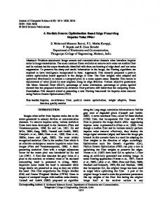
Fig. 11. Construction layout of Jinping-I Hydropower Project.

5 CASE STUDY: THE MULTISTAGE QUEUING DECISION PROBLEM IN CONCRETE TRANSPORTATION SYSTEMS OF JINPING-I HYDROPOWER PROJECT 5.1 Presentation of the case problem An actual large-scale construction project, the Jinping-I Hydropower Project, is used as a practical example to demonstrate the practicality of our modeling approach and the efficacy of the AM-based PSO algorithm. The Jinping-I Hydropower Project is located in the counties of Yanyuan and Muli, Liangshan Yi Autonomous Prefecture, Sichuan Province, China. The project is made up of permanent structures categorized as water retaining, spillway and dissipation, power tunnels and a powerhouse complex. Its 305-m-high double curvature concrete arch dam is the world’s highest dam. The construction layout of the Jinping-I Hydropower Project is shown in Figure 11. The only concrete production system that contains three concrete mixing buildings (i.e., M = 3) is located on the left bank of the dam. There are four (i.e., N = 4) transport paths that connect the concrete production system with its corresponding

Fig. 12. Variation of fitness value with different population size within 100 iterations.

unloading sites. When the concrete is transported to the corresponding unloading site by the vehicles, the cable machines unload the concrete from the vehicles and transport it to the corresponding pouring area. The

790

Zeng, Xu, Wu & Shen

working control area is a rectangle for the parallel mobile type cable machines. Different groups of cable machines that are in charge of different pouring areas are installed at different elevations to avoid mutual interference. 5.2 Data collection Detailed data for the Jinping-I Hydropower Project were obtained from the Ertan Hydropower Development Company, Ltd. The fuzzy data including effective monthly working days and transportation and stay time were obtained from previous data and expert experience. Detailed information is shown in Table 6. Based on Equations (1) and (2), the arrival rate of vehicles (i.e., λ˜ i (k)) can be easily computed and are summarized with the service rates of the cable machines (i.e., μ˜ i (k)) that were obtained from previous data and ˜ expert experience in Table 7. Because ρ˜i (k) = μλ˜ ii (k) , the (k) results of ρ˜i (k) were computed based on the algebraic operations for triangular fuzzy numbers (Xu and Zhou, 2011) and are shown in Table 7. Other important parameters including the initial number of available vehicles and unloading equipment at the first stage (i.e., α1 and β1 ), the equipment failure rates for the vehicles and unloading equipments which are allocated to Subsystem i in Stage k (i.e., ψi (k) and φi (k)), the number of supplemental vehicles and unloading equipment in Stage k + 1 (i.e., RV (k + 1) and R E (k + 1)), the work time (hour/day) of vehicles (i.e., t), the heaped capacity for a vehicle (m3 /vehicle) (i.e., H), the required concrete pouring quantity for Pouring Area i in Stage k (i.e., Q i (k)), the unit operational cost (CNY/day) of a concrete mixing building (i.e., Cb ), the unit operational cost (CNY/day) of a vehicle (i.e., Cv ), the unit operational cost (CNY/day) of a cable machine (i.e., Ce ), and the most endurable construction duration for a transportation system (i.e., D) are presented in Tables 8 and 9. 5.3 Parameters selection for AM-based PSO The PSO parameters are determined based on the results of some preliminary experiments that were carried out to observe the behavior of the algorithm at different parameter settings. From a comparison of several sets of parameters, including the population size, iteration number, acceleration constant, initial velocity, and inertia weight, the most reasonable parameters are identified. Note that the population size (i.e., the number of particles) determines the evaluation runs, and thus impacts the optimization cost (Trelea, 2003). Here, four population size candidates are considered:

30, 40, 50, and 60. The testing iteration number is set as 200. From the results (see Figure 12), it was observed that the AM-based PSO performed poorly with small population sizes (30 and 40). This can be inferred from the fact that the minimum fitness values are larger than the other two population sizes (50 and 60) when the AM-based PSO search operations reach convergence after 50 iterations. A possible reason may be that small population sizes cannot provide a sufficient number of possible layouts for the algorithm. Insufficient resources restrict the search capacity of the algorithm. Although small population sizes can save computational time and ensure the efficiency of the search operation, the final fitness value may not be the smallest. Both 50 and 60 population sizes converge on the same optimal fitness value. Thus, the computation efficiency (time) needs to be used as the evaluation criteria. The best fitness values for each population size are obtained after 50 runs of the algorithm. For 50 and 60 population sizes, it was observed that both have the same best fitness values (52.72 × 106 yuan) and the algorithm search operation with a 60 population size reaches convergence faster than a 50 population size. However, the algorithm search operation with a 60 population size takes more time to search and compute the optimal solution. Although the search operation can possibly reach convergence faster with an increase in population size, the computation times also takes longer. Therefore, a medium population size (50) may be the optimal choice as it can make full use of resources and operate more efficiently. The testing results also indicate that the convergence iteration numbers for most experiments are within 100 times. Because an excess iteration number leads to redundant computations, the iteration number is set at 100. The inertia weight w(τ ) is set to be varying with the iteration as follows: w(τ ) = w(T ) +

τ −T [w(1) − w(T )] 1−T

(28)

where τ is iteration index = 1, 2, . . . , T; T = iteration limit. Through further experiments, w(1) = 1.0 and w(T ) = 0.1 are found to be the most suitable, to control the impact of the previous velocities on the current velocity and to influence the trade-off between the global and local experiences. The other parameters are selected by comparing the results with the observations from the dynamic search behaviors of the swarm. The selection of the acceleration coefficients c p and cg affects both the convergence speed and the ability to escape from the local minima. Initial PSO studies often used c p = cg = 2.0 (van den Bergh and Engelbrecht, 2010). Although good results have been obtained, it was observed that velocities quickly exploded to large values which lead to a slower convergence speed and

AM-based PSO for queuing networks problem

791

Table 6 The data information for the effective monthly working days, transportation and stay time Stage index Model parameters T˜h1 (k) T˜e1 (k) T˜u1 (k) T˜h2 (k) T˜e2 (k) T˜u2 (k) T˜h3 (k) T˜e3 (k) T˜u3 (k) T˜h4 (k) T˜e4 (k) T˜u4 (k) T˜e (k)

k=1

k=2

k=3

Measurement unit

(0.28,0.34,0.40) (0.20,0.25,0.27) (0.19.0.23,0.27) (0.38,0.42,0.47) (0.22,0.27,0.31) (0.17,0.21,0.26) (0.36,0.40,0.44) (0.28,0.33,0.37) (0.18,0.22,0.25) (0.23,0.27,0.34) (0.14,0.21,0.26) (0.19,0.22,0.26) (0.12,0.15,0.19)

(0.30,0.37,0.44) (0.23,0.26,0.29) (0.17,0.21,0.25) (0.40,0.44,0.48) (0.24,0.30,0.35) (0.18,0.23,0.27) (0.37,0.41,0.45) (0.26,0.34,0.39) (0.19,0.23,0.28) (0.25,0.29,0.33) (0.15,0.22,0.27) (0.18,0.23,0.27) (0.11,0.14,0.18)

(0.26,0.32,0.28) (0.18,0.22,0.25) (0.16.0.19.0.23) (0.36,0.40,0.45) (0.20,0.24,0.29) (0.16,0.20,0.25) (0.32,0.37,0.41) (0.22,0.29,0.35) (0.18,0.23,0.26) (0.22,0.27,0.31) (0.13,0.20,0.24) (0.18,0.22,0.25) (0.12,0.14,0.17)

hour hour hour hour hour hour hour hour hour hour hour hour hour

Table 7 The data information for arrival rate of vehicles, service rate of cable machines, and their ratio Stage index Model parameters λ˜ 1 (k) μ˜ 1 (k) ρ˜1 (k) λ˜ 2 (k) μ˜ 2 (k) ρ˜2 (k) λ˜ 3 (k) μ˜ 3 (k) ρ˜3 (k) λ˜ 4 (k) μ˜ 4 (k) ρ˜4 (k)

k=1

k=2

k=3

(0.8850,1.0309,1.2658) (3.7037,4.3478,5.2632) (0.1681,0.2371,0.3418) (0.8130,0.9524,1.1236) (3.8462,4.7619,5.8824) (0.1382,0.2000,0.2921) (0.8000,0.9091,1.0638) (4.0000,4.5455,5.5556) (0.1440,0.2000,0.2660) (0.9524,1.1765,1.4706) (3.8462,4.5455,5.2632) (0.1810,0.2588,0.3824)

(0.8621,1.0204,1.2346) (4.0000,4.7619,5.8824) (0.1466,0.2143,0.3086) (0.7813,0.9009,1.0753) (3.7037,4.3478,5.5556) (0.1406,0.2072,0.2903) (0.7692,0.8929,1.0753) (3.5714,4.3478,5.2632) (0.1462,0.2054,0.3011) (0.9524,1.1364,1.4493) (3.7037,4.3478,5.5556) (0.1714,0.2614,0.3913)

(0.9709,1.1494,1.3889) (4.3478,5.2632,6.2500) (0.1553,0.2184,0.3194) (0.8621,1.0204,1.1905) (4.0000,5.0000,6.2500) (0.1379,0.2041,0.2976) (0.8403,0.9709,1.1905) (3.8462,4.3478,5.5556) (0.1513,0.2233,0.3095) (1.0309,1.2048,1.5385) (4.0000,4.5455,5.5556) (0.1856,0.2651,0.3846)

Note: The measurement unit of λ˜ i (k) and μ˜ i (k) is vehicle/hour.

an inadequate computing stability. In order to avoid being trapped into a local optimal solution and improve the convergence speed, the acceleration coefficients c p and cg are selected based on the comparison of 16 parameter combinations. A sensitivity analysis is performed as shown in Table 10. The results in Table 10 are obtained from 50 runs of the experiment for each combination, and the optimistic–pessimistic index is set as η = 0.5. It can be concluded that the performance of the algorithm can be slightly influenced by a change in the acceleration coefficients c p and cg . Although all combinations are able to obtain the same best fitness value (i.e., 52.72), it appears that with an increase in the acceleration coefficients (both for c p and cg ), there is

also an increasing trend for the worst and average fitness values, the fitness value variance, and the average convergence number and computing time, when c p and cg are both greater than 1.0 (i.e., Combinations 6–16). The reason for this may be explained by the fact that larger acceleration coefficients mean that the velocities are more likely to explode to large values, which will slow down the convergence speed and result in a longer computing time. For the other combinations (Combinations 1–5), because c p and cg are relatively small (either less than 1.0), the search operations are more focused on exploitation rather than exploration, which increases the instability and computation time. From the results shown in Table 10, Combination 6 has the lowest fitness

792

Zeng, Xu, Wu & Shen

Table 8 Estimated quipment failure rates and supplemental number Model parameters Stage index k

ψ1 (k)

ψ2 (k)

ψ3 (k)

ψ4 (k)

φ1 (k)

φ2 (k)

φ3 (k)

φ4 (k)

RV (k)

R E (k)

1 2 3

0.043 0.108 –

0.043 0.108 –

0.043 0.108 –

0.043 0.108 –

0.202 0.168 –

0.202 0.168 –

0.202 0.168 –

0.202 0.168 –

– 10 0

– 2 0

Table 9 Required concrete pouring quantity, work hours per day, vehicle heaped capacity, daily costs and maximum acceptable duration Model parameters αk

βk

Q 1 (k)

Q 2 (k) Q 3 (k) (104 m3 )

Q 4 (k)

t (hour/day)

H (m3 /vehicle)

Cb

48 – –

5 – –

20.75 65.76 29.72

28.62 86.92 40.58

20.48 64.82 28.37

18 18 18

11 11 11

992 992 992

Stage index k 1 2 3

31.34 83.17 37.29

Cv Ce (CNY/day) 551 551 551

1226 1226 1226

D (month) 62 62 62

behavior due to its less search time and more efficient computation. Figure 14 provides the velocity index on a typical run of the AM-based PSO for Combination 6, which shows a good balance between exploration and exploitation which could lead to a good solution. Table 11 summarizes all parameter values selected for the AM-based PSO in our computational experiments.

5.4 Results and sensitivity analysis

Fig. 13. Search behavior of the AM-based PSO for 16 parameter combinations.

value variance (i.e., 0.6073), the smallest average convergence iteration number (i.e., 23), and the shortest average computing time (i.e., 170.094 seconds). Thus, it is appropriate to select Combination 6 as the best acceleration coefficients setting (i.e., c p = 1.0 and cg = 1.0) for the AM-based PSO. The values for the initial velocity are selected based on the empirical conditions described in section “Antithetic particle-updating mechanism”. Figure 13 shows the search behavior of the AM-based PSO for the 16 parameter combinations in Table 10, which indicates that Combination 6 has the best search

To show the practicality and efficiency of the optimization method for the multistage queuing decision problem in the Jinping-I Hydropower Project presented in this article, we implemented the AM-based PSO algorithm to solve the problem previously described, and compared the results with the actual data collected from the Jinping-I Hydropower Project. The results are shown in Table 12, which were obtained based on the following optimistic–pessimistic index, that is, η = 0.5. By comparing the fitness value of total operational cost and the algorithm value for the total construction duration with the actual data from the project in Table 12, our findings indicate that there are differences between the solutions generated by our algorithm and the actual data. The net reduction value for the total operational cost is 4.17 × 106 yuan, and the rate of reduction is 7.33%. The net reduction value for the total construction duration is 3.97 months, and the rate of reduction is 6.91%. This improvement in construction efficiency could bring considerable economic benefit to a construction project, especially a large-scale one. Because

793

Average 54.11 53.87 54.24 54.81 53.37 53.17 53.77 54.03 53.97 53.86 53.92 54.59 54.28 54.17 54.41 54.73 Worst 55.03 54.68 55.29 55.83 54.78 54.48 54.96 55.24 55.12 55.03 55.18 55.68 55.34 55.26 55.53 55.79

Fig. 14. Velocity index on typical run of AM-based PSO for Combination 6. Table 11 Parameter selection for AM-based PSO

w(T) 0.1 0.1 0.1 0.1 0.1 0.1 0.1 0.1 0.1 0.1 0.1 0.1 0.1 0.1 0.1 0.1

Best 52.72 52.72 52.72 52.72 52.72 52.72 52.72 52.72 52.72 52.72 52.72 52.72 52.72 52.72 52.72 52.72

Fitness value (106 yuan)

Population size L

Iteration number T 100

Acceleration coefficient

Inertia weight

cp

cg

w(1)

w(T)

1.0

1.0

1.0

0.1

w(1) 1.0 1.0 1.0 1.0 1.0 1.0 1.0 1.0 1.0 1.0 1.0 1.0 1.0 1.0 1.0 1.0

50

Parameter combination Combination 1 Combination 2 Combination 3 Combination 4 Combination 5 Combination 6 Combination 7 Combination 8 Combination 9 Combination 10 Combination 11 Combination 12 Combination 13 Combination 14 Combination 15 Combination 16

cp 0.5 0.5 0.5 0.5 1.0 1.0 1.0 1.0 1.5 1.5 1.5 1.5 2.0 2.0 2.0 2.0

cg 0.5 1.0 1.5 2.0 0.5 1.0 1.5 2.0 0.5 1.0 1.5 2.0 0.5 1.0 1.5 2.0

Population size L 50 50 50 50 50 50 50 50 50 50 50 50 50 50 50 50

Iteration number T 100 100 100 100 100 100 100 100 100 100 100 100 100 100 100 100

Inertia weight Acceleration coefficient

Table 10 Sensitivity analysis for acceleration coefficients selection of AM-based PSO

Variance 0.7134 0.6589 0.7903 0.8584 0.6658 0.6073 0.6732 0.8216 0.7832 0.7244 0.8045 0.9205 0.9085 0.8832 0.9543 0.9933

Average convergence iteration number 27 25 27 29 24 23 26 28 27 26 29 32 31 30 32 34

Average computing time (s) 185.011 178.548 189.103 201.578 176.956 170.094 183.671 198.335 191.836 185.428 200.669 216.301 213.569 209.228 220.844 231.021

AM-based PSO for queuing networks problem

the model is based on a rigorous consideration of practical situations, and the algorithm’s effectiveness was validated through the computational experiments, to some extent, we can conclude from the results data that the theoretical optimized values for the total operational costs and the construction duration for the decision variables are better than the actual values. This means that the current practice is not optimal. In fact, in current practice, decision makers usually make their decisions on experience only. Because the results come from an application of a specific case study, a general extension of such results (e.g., queuing networks with more transportation paths or vehicles) could be used to provide decision makers with a theoretical optimal vehicle and unloading equipment allocation plan to guide current practice. In fact, it could be deduced that the optimal solution must satisfy the condition: D1 (k)=D2 (k)=D3 (k)=D4 (k) for all stages, that is, the concrete construction duration at Pouring Area i in Stage k are all equal to each other for all stages. It is not hard to understand this conclusion by the following consideration. Suppose solution A satisfies the above condition. If a vehicle is moved from its current transportation path σ to another one ρ to

794

Zeng, Xu, Wu & Shen

Table 12 Results for the multistage queuing decision problem in Jinping-I Hydropower Project Subsystem index i=1 Stage index k 1 2 3

i=2

i=3

v1 (k)

e1 (k)

v2 (k)

e2 (k)

v3 (k)

e3 (k)

v4 (k)

e4 (k)

11 12 11

1 1 1

13 16 15

1 2 2

14 15 14

2 2 2

10 13 12

1 1 1

Total operational cost Fitness value (106 yuan) 52.72

i=4

Total construction duration

Actual data from the project (106 yuan)

Net reduction value (106 yuan)

Rate of reduction

Algorithm value (month)

Actual data from the projct (month)

56.89

4.17

7.33%

53.50

57.47

Table 13 Results of concrete construction duration at Pouring Area i in Stage k Subsystem index

Stage index k

i=1 D1 (k)

i=2 D2 (k)

i=3 D3 (k)

i=4 D4 (k)

1 2 3

11.51 27.43 11.41

12.02 28.43 11.42

12.97 28.82 11.71

11.12 28.18 11.30

form another solution B, it could be found out that the concrete construction duration at Pouring Area σ will increase and the concrete construction duration at Pouring Area ρ will reduce. This will lead to the increase of the length of corresponding stage, and thus make the total operational cost increase. This implies that any other solution is worse than solution A. Table 13 shows the results of Di (k) which are the output of the algorithm. It could be found out that the values of each Di (k) for the same stage are approximate to each other. This is acceptable, because the number of vehicles and unloading equipments can change in the form of discrete integers instead of continuous real numbers. To some extent, the results are consistent with the above theoretical inference and just confirm the validation of the algorithm. In order to gain insight into the selection principle for the optimistic–pessimistic index (i.e., η), a sensitivity analysis was conducted against this parameter (see Table 14). The decision makers can fine-tune this parameter to obtain different solutions under different levels. The solutions reflect different optimistic– pessimistic attitudes for uncertainty. The optimistic– pessimistic index (i.e., η) is used to determine the

Net reduction value Rate of (month) reduction 3.97

6.91%

combined attitude of a decision maker, which is relevant to the total operational cost and construction duration. Table 14 summarizes different fitness values (i.e., total operation cost), total construction durations, and optimal solutions (i.e., the number of vehicles for a specific route and the layout of the unloading equipment) for the case problem with respect to different values of η. As shown in Table 14, the analytical results obtained from the case problem indicate that the optimistic– pessimistic index of the decision maker has a significant impact on the decision with a change in the index. If the parameter η is larger, the fitness value and total construction duration decreases. The parameter η also has an effect on the optimal allocation of resources (i.e., vi (k) and ei (k)). The optimal solution (i.e., the number of vehicles for a specific route and the layout of the unloading equipment) slightly changes when different values for the η parameter are selected (see Table 14). The optimistic–pessimistic parameter should be interpreted according to real-world problems. For this case problem, because the objective is to minimize total operational costs and construction duration over the whole construction process, η = 0 is actually a pessimistic extreme, and η = 1, on the contrary, is actually an optimistic extreme. Thus, when 0 ≤ η < 0.5, the attitudes for the variable could be regarded as pessimistic, and when 0.5 ≤ η ≤ 1, the attitudes for the variable could be regarded as optimistic. Then, the following conclusion can be drawn: the result is more optimistic if the optimistic–pessimistic parameter goes up. Depending on their attitudes, it is the decision makers who ultimately decide the optimal result. The results in Table 14 indicate that if the optimistic– pessimistic index is not less than 0.2, the proposed optimization method could find a better solution for

AM-based PSO for queuing networks problem

795

Table 14 Sensitivity analysis on the optimistic–pessimistic index Subsytem index Optimistic– pessimistic index

i=1

i=2

i=3

i=4

Fitness value (106 yuan)

Total construction duration (month)

Stage index k

v1 (k)

e1 (k)

v2 (k)

e2 (k)

v3 (k)

e3 (k)

v4 (k)

e4 (k)

η=0

58.61

59.48

η = 0.1

57.31

58.17

η = 0.2

56.08

56.92

η = 0.3

54.91

55.73

η = 0.4

54.90

55.72

η = 0.6

51.69

52.45

η = 0.7

50.70

51.45

η = 0.8

49.75

50.48

η = 0.9

48.83

49.56

η = 1.0

47.95

48.66

1 2 3 1 2 3 1 2 3 1 2 3 1 2 3 1 2 3 1 2 3 1 2 3 1 2 3 1 2 3

14 16 12 13 16 12 14 17 16 13 16 15 13 16 13 13 17 14 14 15 16 12 17 16 15 13 16 12 13 14

1 1 1 2 1 1 1 1 1 1 1 1 1 1 1 1 1 1 2 1 1 1 1 1 1 1 1 1 1 1

11 14 12 11 14 13 11 13 12 11 14 12 11 14 12 11 13 12 11 15 12 11 13 12 11 13 12 11 17 14

1 2 2 1 2 2 1 2 2 2 2 3 2 2 1 1 2 2 1 2 2 1 2 2 1 2 1 1 2 2

12 13 16 13 13 15 12 13 12 13 13 13 13 13 15 13 13 14 12 13 12 14 13 12 11 13 12 14 13 12

2 2 2 1 2 1 2 2 2 1 2 1 1 2 2 2 2 2 1 2 2 2 2 2 2 2 2 2 2 2

11 13 12 11 13 12 11 13 12 11 13 12 11 13 12 11 13 12 11 13 12 11 13 12 11 17 12 11 13 12

1 1 1 1 1 2 1 1 1 1 1 1 1 1 2 1 1 1 1 1 1 1 1 1 1 1 2 1 1 1

this problem than the actual operation. This means if the decision maker’s attitude for the fuzzy data is not too pessimistic (i.e., η ≥ 0.2), the optimization method is able to achieve improvements in construction efficiency. Although the mathematical model is formulated with some assumptions, the results of sensitivity analysis show that this improvement is not just an accidental event of occasionality. 5.5 Comparison with results of standard PSO and GA Optimization results for the multistage queuing decision problem at the Jinping-I Hydropower Project using the AM-based PSO are compared with the standard PSO and the standard GA. To carry out the comparisons under a similar environment, the parameters stated in Table 11 are also adopted for the standard PSO; that

is, the population size 50, the iteration number 100, the two acceleration coefficients c p and cg are set at values of 1.0 and 1.0, respectively, the inertia weight is the same as in Equation (28), and w(1) = 1.0 and w(T ) = 0.1. The other parameters and updating mechanism for the standard PSO are selected as follows: (1) initial velocities are taken as the same as for the AMbased PSO and (2) Equation (24) is used for the particle updating. If the final solution is infeasible, the standard PSO algorithm restarts until a feasible solution is found. Similarly, the same population size and iteration number are also adopted for standard GA. The crossover possibility and the mutation possibility for the GA are set as pc = 0.75 and pm = 0.05. The convergence histories (Figure 15) are based on the best result from 50 runs of the experiments (for AM-based PSO, standard PSO, and standard GA, respectively).

796

Zeng, Xu, Wu & Shen

Table 15 Comparison results between the AM-based PSO, the standard PSO, and the GA Convergence iteration number

Fitness value

Approach AM-based PSO Standard PSO Standard GA

Computing time (seconds)

Sample size

Minimal

Average

Standard deviation

Average

Standard deviation

Average

Standard deviation

50 50 50

52.72 54.84 52.72

53.17 58.96 56.58

0.7793 1.0232 1.2135

23 79 83

2.3212 2.9872 4.3576

170.094 2654.072 3105.469

12.5432 15.2342 21.8336

significance levels for α are considered to be 0.05 in all cases. The hypothesis for the F-test is as follows: H0κ : σ A2 κ = σ S2κ ;

Fig. 15. Convergence histories of AM-based PSO, standard PSO, and standard GA.

for κ = 1, 2, 3, where H0κ and H1κ are null hypothesis and alternative hypothesis for the F-test, respectively; σ A2 κ and σ S2κ are the variances of fitness values (i.e., κ = 1), the convergence iteration numbers (i.e., κ = 2), and the computing times (i.e, κ = 3) for the AM-based PSO and the standard PSO. When α = 0.05, the rejection κ (49, 49)}. Because region for H0κ is Wκ = {Fκ > F1−α /2 / Wκ for κ = 1, 2, 3, thus the null hypothesis H0κ (for Fκ ∈ κ = 1, 2, 3) is not rejected, that is, the assumption that the fitness variance values, the convergence iteration numbers, and the computing times for the AM-based PSO and the standard PSO are equal can be considered to be true under the significance level α = 0.05. Similarly, the hypotheses for the t-test are as follows: H0∗κ : γ Aκ = γ Sκ ;

Table 15 shows the comparison results obtained from 50 runs (i.e., sample size) for the AM-based PSO, the standard PSO, and the standard GA, respectively, including the minimal, average, and sample standard deviation for the fitness value, the average and sample standard deviation for the convergence iteration number and the computing times. It can be seen that the AM-based PSO is able to search for the same global optima as the standard GA and is faster than the standard PSO. It also has a better computational stability compared to the standard PSO and the standard GA. To detect if there are statistically significant differences in performance between the AM-based PSO and the standard PSO, the t-test statistic (Livingston, 2004) is employed here. Because the t-test can only be used if the variances of the two sample groups are also assumed to be equal, the F-test (Lomax, 2007) is used first to ensure that the fitness values variances, the convergence iteration numbers, and the computing times for the AM-based PSO and the standard PSO are equal. The test results are shown in Table 16, where the

H1κ : σ A2 κ = σ S2κ

H1∗κ : γ Aκ = γ Sκ

for κ = 1, 2, 3, where H0∗κ and H1∗κ are the null hypothesis and alternative hypothesis for the t-test, respectively; γ Aκ and γ Sκ are fitness value means (i.e., κ = 1), the convergence iteration numbers (i.e., κ = 2), and the computing times (i.e, κ = 3) for the AM-based PSO and the standard PSO. When α = 0.05, the rejection region κ (98)}. Because tκ ∈ Wκ∗ for of H0∗κ is Wκ∗ = {|tκ | > t1−α /2 κ = 1, 2, 3, thus the null hypothesis H0∗κ (for κ = 1, 2, 3) is rejected, that is, there are statistically significant differences between the fitness value means (i.e., κ = 1), the convergence iteration numbers (i.e., κ = 2), and the computing times (i.e, κ = 3) for the AM-based PSO and the standard PSO under the significance level α = 0.05. From the comparison results shown in Tables 15 and 16, it can be concluded that there is a statistically significant improved computational efficiency for the AM-based PSO compared with the standard PSO. The reason for the improvements can be explained as follows. If the infeasible solution cannot be avoided, the standard PSO will restart when the final output is an infeasible solution (i.e., the constraints in the model

AM-based PSO for queuing networks problem

797

Table 16 Statistical significance test between the AM-based PSO and the standard PSO Statistical significance test F-test Performance item Fitness value Convergence iteration number Computing time

Index κ

Significance level α

Sample size

Fκ

1 2 3

0.05 0.05 0.05

50 50 50

1.7239 1.6562 1.4751

can not be satisfied) until a feasible solution is found. Because the model has complex constraints, and the updating is performed independently among the elements of a multidimensional particle in the standard PSO, these largely reduce the probability of finding a feasible solution. This means the standard PSO may continually restart a lot of times before it can output a feasible solution which will lead to a much longer computation time and reduce the efficiency and stability of the algorithm as compared with the AM-based PSO. By employing the antithetic particle-updating mechanism, the AMbased PSO maintains the feasibility of the particle positions during the entire particle-updating process, which naturally improves the efficiency of the algorithm by avoiding the infeasible solution search space.

6 CONCLUSIONS AND FUTURE RESEARCH In this article, a closed multi-class queuing network problem with fuzzy data in a concrete transportation system, which is generalized from a prototype of the Jinping-I Hydropower Project, is studied, and a multiple objective decision-making model is established to improve construction efficiency by minimizing both total operational costs and construction duration. Different from a manufacturing queuing problem, the decision maker needs to allocate a limited number of vehicles and unloading equipment to different transportation paths in the queuing network to minimize the total operational costs and construction duration. Because of uncontrollable factors, the effective monthly working days, transportation, stay and waiting time, arrival rate of vehicles and the unloading equipment service rate are characterized as triangular fuzzy numbers. To deal with the fuzzy data, a fuzzy expected value operator with optimistic–pessimistic index is introduced and its equivalent crisp model derived. The particular nature of the model motivates the development of an AM-based PSO algorithm that automatically controls

κ F1−α (49, 49) /2 1.81 1.81 1.81

t-test tκ −31.8307 −104.6729 −890.0914

κ t1−α (98) /2 1.991 1.991 1.991

the particle-updating in the feasible solution space for the equivalent crisp model. Results and a sensitivity analysis for the Jinping-I Hydropower Project are presented to highlight the performance of our optimization method, which is proved to be very effective and efficient compared to other metaheuristic algorithms. The computational results show that the proposed optimization method has made noticeable improvements in the construction efficiency compared to the actual data collected from the Jinping-I Hydropower Project (7.33% reduction for total operational cost, and 6.91% reduction for total construction duration). By comparing the AM-based PSO with other metaheuristic algorithms, the results show that the AM-based PSO has significant advantages in computing efficiency, speed, and stability compared with the standard PSO and the standard GA, as it does not lead to combinatorial explosions or problem-dependent ineffective searches. Similar to the standard GA, it is able to search for global optima and is faster than the standard PSO. However, unlike the standard GA, which needs to predefine the crossover probability and perform crossover between two unclassified survivors or individuals, the AM-based PSO normalizes the particle velocity to represent the probability that a particle will be selected for updating, instead of using the velocity directly to update the particle as in the standard PSO, and designs original and antithetic elements to perform a new particle-updating mechanism. The “one-way” sharing of the local best and the global best experiences during the search process also contributes to the AM-based PSO’s advantages over the standard GA. By applying the AM-based PSO in optimizing the queuing network problem in concrete transportation systems, this study actually opens an application area for the PSO in the construction field. Based on the analysis of the model (i.e., Equation (19)), maximizing the numbers of concrete mixing buildings, the vehicles, and the unloading equipment will lead to a highest operational cost per month,

798

Zeng, Xu, Wu & Shen

but a shortest duration for each stage. Thus, the total operational cost may be optimal if the decreasing of the duration for each stage is stronger than the increasing of the operational cost per month. Otherwise, the total operational cost may be the worst one. In the Jinping-I Hydropower Project, the numbers of concrete mixing buildings, the vehicles, and the unloading equipment are predetermined based on the estimation and experience of the engineers. The limiting factors include the overcrowding on the truck routes, the space needed for concrete mixing, and the allowable carrying capacity of cable machine transition system. The solution that finds the strongest restriction and adapts the other controls accordingly to realize the shortest duration must make the unloading equipment busy all the time without waiting for vehicles coming. How to determine the corresponding maximal numbers of vehicles and concrete mixing buildings to avoid overcrowding on the transportation paths and excessive costs needs further investigation of relevant data and could be an interesting topic in the future research. In practice, data information obtained during construction process is helpful to improve the estimators and reduce uncertainty possibly leading to better solutions. In order to realize continuous optimization for the queuing network problem, the required data should be monitored or measured in each month during the entire concrete construction process. And the parameters in the model could be adjusted or updated in each month based on the data obtained in the previous months to optimize the allocation for the remaining concrete construction task. How to monitor or measure the required data for model updating and establish the framework for continuous optimization could also be an interesting and urgent topic for the future research.

ACKNOWLEDGMENTS This research was supported by the Key Program of NSFC (Grant No. 70831005), “985” Program of Sichuan University “Innovative Research Base for Economic Development and Management”, the Research Foundation of Ministry of Education for the Doctoral Program of Higher Education of China (Grant No. 20130181110063), and China Scholarship Council (CSC) (Grant No. 201206240138). We would like to give our great appreciation to the editors and anonymous referees for their helpful and constructive comments and suggestions, which have helped to improve this article.

REFERENCES Abramov, V. M. (2001), Some results for large closed queuing networks with and without bottleneck: up- and downcrossings approach, Queuing Systems, 38(2), 149–84. Adeli, H. & Hung, S. L. (1995), Machine Learning—Neural Networks, Genetic Algorithms, and Fuzzy Systems, John Wiley and Sons, New York. Adeli, H. & Jiang, X. (2003), Neuro-fuzzy logic model for freeway work zone capacity estimation, Journal of Transportation Engineering, 129(5), 484–93. Adeli, H. & Karim, A. (1997), Scheduling cost optimization and neural dynamics model for construction, Journal of Construction Engineering and Management, 123(4), 450–58. Adeli, H. & Karim, A. (2000), Fuzzy-wavelet RBFNN model for freeway incident detection, Journal of Transportation Engineering, 126(6), 464–71. Adeli, H. & Wu, M. Y. (1998), Regularization neural network for construction cost estimation, Journal of Construction Engineering and Management, 124(1), 18–24. Amiri, G. G., Rad, A. A., Aghajari, S. & Hazaveh, N. K. (2012), Generation of near-field artificial ground motions compatible with median-predicted spectra using PSObased neural network and wavelet analysis, ComputerAided Civil and Infrastructure Engineering, 27(9), 711–30. Anghinolfi, D. & Paolucci, M. (2009), A new discrete particle swarm optimization approach for the single-machine total weighted tardiness scheduling problem with sequencedependent setup times, European Journal of Operational Research, 193, 73–85. Balsamo, S., Persone, V. D. & Inverardi, P. (2003), A review on queuing network models with finite capacity queues for software architectures performance prediction, Performance Evaluation, 51(2–4), 269–88. Bliemer, M. (2007), Dynamic queuing and spillback in an analytical multiclass dynamic network loading model, Transportation Research Record, 2029, 14–21. ´ P. (2013), A particle swarm opBolat, B., Altun, O. & Cortes, timization algorithm for optimal car-call allocation in elevator group control systems, Applied Soft Computing, 13(5), 2633–42. Casale, G. (2011), A generalized method of moments for closed queuing networks, Performance Evaluation, 68(2), 180–200. Chen, S. P. (2007), Solving fuzzy queuing decision problems via a parametric mixed integer nonlinear programming method, European Journal of Operational Research, 177(1), 445–57. Clerc, M. & Kennedy, J. (2002), The particle swarm: explosion, stability, and convergence in a multidimensional complex space, IEEE Transactions on Evolutionary Computation, 6(1), 58–73. Daduna, H. & Szekli, R. (2002), Conditional job-observer property for multitype closed queuing networks, Journal of Applied Probability, 39(4), 865–81. De Vuyst, S., Wittevrongel, S. & Bruneel, H. (2002), Mean value and tail distribution of the message delay in statistical multiplexers with correlated train arrivals, Performance Evaluation, 48(1–4), 103–29. Dubois, D. & Prade, H. (1978), Operations on fuzzy numbers, International Journal of System Sciences, 9, 613–26. Dubois, D. & Prade, H. (1988), Possibility Theory: An Approach to Computerized Processing of Uncertainty, Plenum, New York.

AM-based PSO for queuing networks problem

Dubois, D. & Prade, H. (2012), Gradualness, uncertainty and bipolarity: making sense of fuzzy sets, Fuzzy Sets and Systems, 192(1), 3–24. Eberhart, R. C. & Shi, Y. (2001), Tracking and optimizing dynamic systems with particle swarms, in Proceedings of the IEEE Congress on Evolutionary Computation, Seoul, South Korea, May 27–30, 2001, 1 and 2, 94–97. ` Fougeres, A. J. & Ostrosi, E. (2013), Fuzzy agent-based approach for consensual design synthesis in product configuration, Integrated Computer-Aided Engineering, 20(3), 259– 74. Garvin, M. J. & Cheah, C. Y. J. (2004), Valuation techniques for infrastructure investment decisions, Construction Management and Economics, 22(4), 373–83. George, D. K. & Xia, C. H. (2011), Fleet-sizing and service availability for a vehicle rental system via closed queuing networks, European Journal of Operational Research, 211(1), 198–207. Gerasimov, A. I. (2000), Synthesis of closed queuing networks with several classes of messages on the basis of their optimization and balancing, Cybernetics and Systems Analysis, 36(6), 906–15. Ghosh-Dastidar, S. & Adeli, H. (2006), Neural networkwavelet microsimulation model for delay and queue length estimation at freeway work zones, Journal of Transportation Engineering, 132(4), 331–41. Govil, M. K. & Fu, M. C. (1999), Queuing theory in manufacturing: a survey, Journal of Manufacturing Systems, 18(3), 214–40. Harrison, P. G. & Coury, S. (2002), On the asymptotic behaviour of closed multi-class queuing networks, Performance Evaluation, 47(2–3), 131–38. Holland, J. (1992), Adaptation in Natural and Artificial Systems, MIT Press, Cambridge. Il Choi, D., Kim, T. S. & Lee, S. (2007), Analysis of a queuing system with a general service scheduling function, with applications to telecommunication network traffic control, European Journal of Operational Research, 178(2), 463–71. Ivnitski, V. A. (2001), Network of single-server queues with dependent service times, Queuing Systems, 37(4), 363– 77. Jiang, X. & Adeli, H. (2003), Fuzzy clustering approach for accurate embedding dimension identification in chaotic time series, Integrated Computer-Aided Engineering, 10(3), 287– 302. Jiang, X. M. & Adeli, H. (2004), Object-oriented model for freeway work zone capacity and queue delay estimation, Computer-Aided Civil and Infrastructure Engineering, 19(2), 144–56. Karim, A. & Adeli, H. (2003), Radial basis function neural network for work zone capacity and queue estimation, Journal of Transportation Engineering, 129(5), 494– 503. Kennedy, J. & Eberhart, R. C. (1995), Particle swarm optimization, in Proceedings of the IEEE International Conference on Neural Networks (ICNN 95), Perth, Australia, Nov. 27–Dec. 1, 1995, 1–6, 1942–48. Khare, A. & Rangnekar, S. (2013), A review of particle swarm optimization and its applications in Solar Photovoltaic system, Applied Soft Computing, 13(5), 2997–3006. Kim, B. J., Kim, W. & Song, B. H. (2008), Sequencing and scheduling highway network expansion using a discrete network design model, The Annals of Regional Science, 42(3), 621–42.

799

Kim, S. (2009), The toll plaza optimization problem: design, operations, and strategies, Transportation Research Part ELogistics and Transportation Review, 45(1), 125–37. Kirkpatrick, S., Gelatt, C. D. & Vecchi, M. P. (1983), Optimization by simulated annealing, Science, 220(4598), 671– 80. Kogan, Y. (2002), Asymptotic expansions for large closed and loss queuing networks, Mathematical Problems in Engineering, 8(4–5), 323–48. Kumar, V. & Singh, T. P. (2007), On linkage of queues in semi-series to a flow-shop scheduling system, International Journal of Agricultural and Statistical Sciences, 3(2), 571– 80. Lee, D. M. & Donnell, E. T. (2006), Analysis of nighttime driver behavior and pavement marking effects using fuzzy inference system, Journal of Computing in Civil Engineering, 21(3), 200–10. Lee, D. M., Pietrucha, M. T. & Donnell, E. T. (2006), Incorporation of transportation experts’ opinions of median safety using a hierarchical fuzzy inference system, Transportation Research Record, 1961, Transportation Research Board, Washington DC. Liu, F. & Er, M. J. (2012), A novel efficient learning algorithm for self-generating fuzzy neural network with applications, International Journal of Neural Systems, 22(1), 21–35. Livingston, E. H. (2004), Who was student and why do we care so much about his t-test? Journal of Surgical Research, 118, 58–65. Lomax, R. G. (2007), Statistical Concepts: A Second Course. Routledge, New York. Mohan, B. C. & Baskaran, R. (2012), A survey: ant colony optimization based recent research and implementation on several engineering domain, Expert Systems with Applications, 39(4), 4618–27. Nahmias, S. (1978), Fuzzy variables, Fuzzy Sets and Systems, 1, 97–110. Nemhanser, G. L. & Wolsey, L. A. (1988), Integer and Combinatorial Optimization, John Wiley and Sons, New York. Nyirenda, C. N., Dawoud, D. S., Dong, F., Negnevitsky, M. & Hirota, K. (1978), A fuzzy multiobjective particle swarm optimized TS fuzzy logic congestion controller for wireless local area networks, Journal of Advanced Computational Intelligence and Intelligent Informatics, 15(1), 41–54. Papadopoulos, H. T. (1996), A field service support system using a queuing network model and the priority MVA algorithm, Omega, 24(2), 195–203. Papadopoulos, H. T. & Heavey, C. (1996), Queuing theory in manufacturing systems analysis and design: a classification of models for production and transfer lines, European Journal of Operational Research, 92(1), 1–27. Plevris, V. & Papadrakakis, M. (2011), A hybrid particle swarm-gradient algorithm for global structural optimization, Computer-Aided Civil and Infrastructure Engineering, 26(1), 48–68. Puterman, M. L. (2005), Markov Decision Processes: Discrete Stochastic Dynamic Programming, John Wiley & Sons, Inc., Hoboken, NJ. Putha, R., Quadrifoglio, L. & Zechman, E. (2012), Comparing ant colony optimization and genetic algorithm approaches for solving traffic signal coordination under oversaturation conditions, Computer-Aided Civil and Infrastructure Engineering, 27(1), 14–28. Rahmati, S. H. A. & Pasandideh, S. H. R. (2012), A fuzzy approach to queuing system’s measures and steadiness,

800

Zeng, Xu, Wu & Shen

Economic Computation and Economic Cybernetics Studies and Research, 46(1), 233–49. Rana S., Jasola, S. & Kumar, R. (2011), A review on particle swarm optimization algorithms and their applications to data clustering, Artificial Intelligence Review, 35(3), 211–22. Sarma, K. C. & Adeli, H. (2001), Bilevel parallel genetic algorithms for optimization of large steel structures, ComputerAided Civil and Infrastructure Engineering, 16(5), 295–304. Shafahi, Y. & Bagherian, M. (2013), A customized particle swarm method to solve highway alignment optimization problem, Computer-Aided Civil and Infrastructure Engineering, 28(1), 52–67. Shi, Y. & Eberhart, R. C. (1998), Parameter selection in particle swarm optimization, in Proceedings of the 7th International Conference on Evolutionary Programming (EP98), San Diego, CA, Mar. 25–27, 1998, 591–600. Subramanian, K. & Suresh, S. (2012), Human action recognition using meta-cognitive neuro-fuzzy inference system, International Journal of Neural Systems, 22(6), 1250028, DOI: 10.1142/S0129065712500281. Szeto, W. Y., Jiang, Y. & Sumalee, A. (2011), A cell-based model for multi-class doubly stochastic dynamic traffic assignment, Computer-Aided Civil and Infrastructure Engineering, 26(8), 595–611. Theodoridis, D., Boutalis, Y. & Christodoulou, M. (2012), Dynamical recurrent neuro-fuzzy identification schemes employing switching parameter hopping, International Journal of Neural Systems, 22(2), 1250004, DOI: 10.1142/S0129065712500049. Tian, W. W. & Zhang, L. S. (2004), An algorithm for finding global minimum of nonlinear integer programming, Journal of Computational Mathematics, 22(1), 69–78. Trelea, I. C. (2003), The particle swarm optimization algorithm: convergence analysis and parameter selection, Information Processing Letters, 85(6), 317–25. Vakharia, A. J., Moily, J. P. & Huang, Y. (1999), Evaluating virtual cells and multistage flow shops: an analytical approach, International Journal of Flexible Manufacturing Systems, 11(3), 291–314. Van, W. T. & Vandaele, N. (2007), Modeling traffic flows with queuing models: a review, ASIA-Pacific Journal of Operational Research, 24(4), 435–61. van den Bergh, F. & Engelbrecht, A. P. (2010), A convergence proof for the particle swarm optimiser, Fundamenta Informaticae, 105, 341–74. Vitins, B. J. & Axhausen, K. W. (2009), Optimization of large transport networks using the ant colony heuristic, Computer-Aided Civil and Infrastructure Engineering, 24(1), 1–14.

Wang, W. X., Shang, Y. L. & Zhang, L. S. (2011), Identifying a global optimizer with filled function for nonlinear integer programming, Discrete Dynamics in Nature and Society, Doc No: 171697. Wang, T., Wang, G. N. & Liu, K. (2009), Simulation control of concrete pump truck boom based on PSO and adaptive robust PD, in 2009 Chinese Control and Decision Conference (CCDC 2009), Guilin, China, June 17–19, 2009, 960–63. Xu, J. P. & Zeng, Z. Q. (2011), Applying optimal control model to dynamic equipment allocation problem: case study of concrete-faced rockfill dam construction project, Journal of Construction Engineering and ManagementASCE, 137(7), 536–50. Xu, J. P. & Zeng, Z. Q. (2012), A discrete time optimal control model with uncertainty for dynamic machine allocation problem and its application to manufacturing and construction industries, Applied Mathematical Modelling, 36(8), 3513–44. Xu, J. P. & Zhou, X. (2011), Fuzzy-Like Multiple Objective Decision Making, Springer-Verlag, Berlin, Heidelberg. Yan, L. & Ma, Z. M. (2012a), Comparison of entity with fuzzy data types in fuzzy object-oriented databases, Integrated Computer-Aided Engineering, 19(2), 199–212. Yan, L. & Ma, Z. M. (2012b), Incorporating fuzzy information into the formal mapping from web data model to extended entity-relationship model, Integrated Computer-Aided Engineering, 19(4), 313–30. Yan, L. & Ma, Z. M. (2013), Conceptual design of objectoriented databases for fuzzy engineering information modeling, Integrated Computer-Aided Engineering, 20(2), 183– 97. Yapicioglu, H., Smith, A. E. & Dozier, G. (2007), Solving the semi-desirable facility location problem using bi-objective particle swarm, European Journal of Operational Research, 177, 733–49. Zadeh, L. A. (1965), Fuzzy sets, Information and Control, 8, 338–53. Zeferino, J. A., Antunes, A. P. & Cunha, M. C. (2009), An efficient simulated annealing algorithm for regional wastewater system planning, Computer-Aided Civil and Infrastructure Engineering, 24(5), 359–70. Zhang, H., Li, H. & Tam, C. M. (2006a), Permutationbased particle swarm optimization for resource-constrained project scheduling, Journal of Computing in Civil Engineering, 20(2), 141–49. Zhang, H., Tam, C. M. & Li, H. (2006b), Multimode project scheduling based on particle swarm optimization, Computer-Aided Civil and Infrastructure Engineering, 21(2), 93–103.