This article was downloaded by: [Clemson University] On: 25 November 2014, At: 19:01 Publisher: Taylor & Francis Informa Ltd Registered in England and Wales Registered Number: 1072954 Registered office: Mortimer House, 37-41 Mortimer Street, London W1T 3JH, UK
Mechanics of Advanced Materials and Structures Publication details, including instructions for authors and subscription information: http://www.tandfonline.com/loi/umcm20
A Resource Allocation Framework for Experimentbased Validation of Numerical Models a
a
S. Atamturktur Assistant Professor , J. Hegenderfer Former Ph.D. Student , B. Williams b
a
Technical Staff Member CS-Division , M. Egeberg Graduate Student , R.A. Lebensohn b
Technical Staff Member MTS-Division & C. Unal Technical Staff Member D-Division a
b
Glenn Department of Civil Engineering, Clemson University, SC, 29634, USA
b
Los Alamos National Laboratory, Los Alamos, NM 87545, USA Accepted author version posted online: 30 Jun 2014.
To cite this article: S. Atamturktur Assistant Professor, J. Hegenderfer Former Ph.D. Student, B. Williams Technical Staff Member CS-Division, M. Egeberg Graduate Student, R.A. Lebensohn Technical Staff Member MTS-Division & C. Unal Technical Staff Member D-Division (2014): A Resource Allocation Framework for Experiment-based Validation of Numerical Models, Mechanics of Advanced Materials and Structures, DOI: 10.1080/15376494.2013.828819 To link to this article: http://dx.doi.org/10.1080/15376494.2013.828819
Disclaimer: This is a version of an unedited manuscript that has been accepted for publication. As a service to authors and researchers we are providing this version of the accepted manuscript (AM). Copyediting, typesetting, and review of the resulting proof will be undertaken on this manuscript before final publication of the Version of Record (VoR). During production and pre-press, errors may be discovered which could affect the content, and all legal disclaimers that apply to the journal relate to this version also.
PLEASE SCROLL DOWN FOR ARTICLE Taylor & Francis makes every effort to ensure the accuracy of all the information (the “Content”) contained in the publications on our platform. However, Taylor & Francis, our agents, and our licensors make no representations or warranties whatsoever as to the accuracy, completeness, or suitability for any purpose of the Content. Any opinions and views expressed in this publication are the opinions and views of the authors, and are not the views of or endorsed by Taylor & Francis. The accuracy of the Content should not be relied upon and should be independently verified with primary sources of information. Taylor and Francis shall not be liable for any losses, actions, claims, proceedings, demands, costs, expenses, damages, and other liabilities whatsoever or howsoever caused arising directly or indirectly in connection with, in relation to or arising out of the use of the Content. This article may be used for research, teaching, and private study purposes. Any substantial or systematic reproduction, redistribution, reselling, loan, sub-licensing, systematic supply, or distribution in any form to anyone is expressly forbidden. Terms & Conditions of access and use can be found at http:// www.tandfonline.com/page/terms-and-conditions
ACCEPTED MANUSCRIPT A Resource Allocation Framework for Experiment-based Validation of Numerical Models S. Atamturktur1, J. Hegenderfer 2, B. Williams3, M. Egeberg4, R.A. Lebensohn5, and C. Unal6 Abstract In experiment-based validation, uncertainties and systematic biases in model predictions are reduced by either increasing the amount of experimental evidence available for model
Downloaded by [Clemson University] at 19:01 25 November 2014
calibration—thereby mitigating prediction uncertainty—or increasing the rigor in the definition of physics and/or engineering principles—thereby mitigating prediction bias. Hence, decision makers must regularly choose between either allocating resources for experimentation or further code development. The authors propose a decision-making framework to assist in resource allocation strictly from the perspective of predictive maturity and demonstrate the application of this framework on a non-trivial problem of predicting the plastic deformation of polycrystals. Keywords: Bayesian Inference; Model Calibration, Uncertainty Quantification; Predictive Maturity; Viscoplastic Self-Consistent; Material Plasticity Models
1
Corresponding author: Assistant Professor, Glenn Department of Civil Engineering, Clemson University, SC, 29634, USA. E-mail address:
[email protected] 2 Former Ph.D. Student, Glenn Department of Civil Engineering, Clemson University, SC, 29634, USA 3 Technical Staff Member, CS-Division, Los Alamos National Laboratory, Los Alamos, NM 87545, USA 4 Graduate Student, Glenn Department of Civil Engineering, Clemson University, SC, 29634, USA 5 Technical Staff Member, MTS-Division, Los Alamos National Laboratory, Los Alamos, NM 87545, USA 6 Technical Staff Member, D-Division, Los Alamos National Laboratory, Los Alamos, NM 87545, USA
1
ACCEPTED MANUSCRIPT
ACCEPTED MANUSCRIPT INTRODUCTION Numerical models are approximate representations of real-world phenomena and thus, simulations invariably suffer from a degree of inaccuracy and imprecision that can be attributed to (i) incomplete modeling of physics and/or engineering principles, (ii) imprecisely known model input parameters, and (iii) numerical uncertainties incurred while solving the
Downloaded by [Clemson University] at 19:01 25 November 2014
mathematical equations [1,2] Incomplete modeling of physics and/or engineering principles, the first factor, refers to the physical phenomena that are either completely unforeseen or that are known, but too complex to incorporate in the model. This incompleteness invariably causes systematic bias in predictions [3-7] and often leads to missing input parameters [8]. Imprecise model parameters, the second factor, are identified by the analyst; however, their precise values (or distributions) remain unknown [9,10]. These imprecise model parameters are typically the main contributors to the uncertainty in predictions. Numerical uncertainties, the third factor, can be treated by code and solution verification activities that ensure the mathematical equations are solved correctly [1113]. Verification is a prerequisite to experiment-based validation [14] and thus, the third factor, which involves numerical uncertainties, is excluded from the scope of the present paper. The primary aim of the model developer then becomes one of reducing the parameter uncertainty and systematic bias in model predictions. These objectives can be achieved by allocating resources to either (i) undertake experimentation to increase the number of physical observations used in the model calibration process or (ii) code development to improve the manner, in which physics and/or engineering principles are defined. Expanding the experimental campaign by conducting new experiments can reduce parameter uncertainty and produce a more
2
ACCEPTED MANUSCRIPT
ACCEPTED MANUSCRIPT refined estimate of systematic bias; while improvement in the description of physics and/or engineering principles can lead to a reduction in the systematic bias. An improved, more detailed model may however, lead to a higher number of uncertain input parameters, and increase the prediction uncertainty [8]. Thus, reducing prediction uncertainty and prediction bias are often conflicting objectives [15]. Therefore, the relative benefits of these two routes, further
Downloaded by [Clemson University] at 19:01 25 November 2014
experimentation versus further code development, vary depending upon available experimental measurements and the existing predictive capability of the numerical model. Considering the finite resources, effectively choosing one approach over the other becomes an issue of efficient allocation of available resources. By focusing on the relative benefits of each approach strictly from the perspective of predictive capability, the authors propose a resource allocation framework that aids in the selection between further experimentation and code development. The application of this proposed framework is demonstrated on the viscoplastic self-consistent (VPSC) material code for modeling plastic deformation. RESOURCE ALLOCATION FRAMEWORK Fig. 1 illustrates the proposed framework, which begins with an initial numerical model and a starting set of physical measurements. This initial model is imprecise due to parameter uncertainties and thus, must be calibrated against experiments. Such calibration is possible using a variety of back-calculation techniques. In this study, a statistical inference procedure originally proposed by Kennedy and O’Hagan [7] and formulated into a standard model calibration procedure by Higdon et al. [5] is adopted. This calibration procedure conditions the probability distributions of input parameters to the experimental evidence reducing the uncertainties in the input parameters, and thus leading to a reduction in prediction uncertainty. An increased
3
ACCEPTED MANUSCRIPT
ACCEPTED MANUSCRIPT availability of experiments results in a greater reduction in prediction uncertainty. In the framework proposed herein, this reduction is traced by quantifying the information gained using an entropy-based metric. Aside from prediction uncertainty, the initial numerical model in Fig. 1 also has a prediction bias, i.e. fundamental inability to reproduce the reality that cannot be remedied solely by
Downloaded by [Clemson University] at 19:01 25 November 2014
calibrating the input parameters. According to Kennedy and O’Hagan [7], prediction bias can be determined by quantifying the deviations between the experiments and the model predictions obtained with ‘best fitted’ parameter values. Since experiments are only available at discrete settings, empirically training an error model becomes necessary to estimate the systematic bias at the untested settings [5]. As more experiments become available, the prediction bias can be estimated with greater fidelity, ultimately converging to the “true” bias of the model. In the framework proposed herein, the convergence of prediction bias is traced by calculating an averaged bias for the entire domain of applicability through the independently trained, empirical error model, henceforth referred to as discrepancy. At the decision node in the framework, the decision maker must assess the predictive capability of the numerical model by evaluating the stabilization of the discrepancy and the information gain metrics throughout the domain of applicability. For a sound model developed based on well-founded physics or engineering principles, the absence of stabilization of the information gain metric indicates that the prediction uncertainty has not yet been fully mitigated, while the absence of stabilization of the discrepancy indicates that prediction bias has not yet been properly defined. In this case, resources must be allocated for experimentation. Poorly built models fail to exhibit stabilization in discrepancy even after a significant number of experiments
4
ACCEPTED MANUSCRIPT
ACCEPTED MANUSCRIPT are conducted; therefore, at this point in the framework, a measure of how well the current experiments explore the domain of applicability (referred to as coverage) is compared to a maximum coverage limit [16-18]. Exceeding the maximum coverage limit without stabilization indicates that the model is too crude for its purposes and resources must be allocated for code development.
Downloaded by [Clemson University] at 19:01 25 November 2014
If stabilization is observed, however, then the ability of the available experiments to sufficiently explore the domain is analyzed. Stabilization when only a small portion of the domain is explored by experiments cannot ensure that the prediction bias is properly defined throughout the entire domain. Therefore, a minimum coverage limit needs to be reached; otherwise more experiments must be conducted to explore the domain of applicability. If stabilization is observed, and the minimum coverage threshold is met, then the epistemic component of parameter uncertainty can be expected to be adequately reduced, and the inferred prediction bias can be considered a proper representation of the incompleteness and inexactness of the model. In this case, further experimentation would only marginally improve the inference of the systematic bias, and allocating resources to experiments cannot be justified. The decision maker must then evaluate if the remaining prediction bias is at an acceptably low level for the application of interest. If the prediction bias is sufficiently low, the model is considered valid for the particular application. If the prediction bias is unacceptably high for the specific purposes of model predictions, the physics and/or engineering principles in the model must be improved. An improved model may have a larger number of uncertain parameters and may require a more extensive experimental campaign to mitigate the increased prediction uncertainty [8]. Therefore,
5
ACCEPTED MANUSCRIPT
ACCEPTED MANUSCRIPT it becomes necessary to check the stabilization of both information gain metric and discrepancy simultaneously. The framework in Fig. 1 therefore loops through the aforementioned steps until the formulated discrepancy and information gain metrics converge to the acceptable levels. METRICS FOR PREDICTION UNCERTAINTY AND BIAS Prediction Uncertainty: Information gain
Downloaded by [Clemson University] at 19:01 25 November 2014
As the information gain is equal to the amount of uncertainty removed, entropy, defined as a measure of uncertainty, is equivalent to the amount of information [19]. Herein, an information gain metric based on Shannon entropy is utilized to quantify the prediction uncertainty as additional experiments become available to condition the posterior distributions of input parameters. For a discrete random variable, z, with a probability mass function, p(z), the entropy is expressed as: H z p ( z ) log p ( z )
(1)
zZ
where the logarithm to base 2 is used to measure entropy in bits and z represents the calibrated model predictions. As an increasing number of experiments are used in the calibration process, the information gain metric, expressed in percentages, is calculated using the following relationship:
H H expt(i) Info-Gain(i)(%) ref H ref
*100
(2)
where H ref is the entropy calculated for the model predictions obtained with the initial distributions of the calibration parameters prior to the availability of experiments. H expt(i) is the
6
ACCEPTED MANUSCRIPT
ACCEPTED MANUSCRIPT entropy of the calibrated model predictions, in which i is the number of experiments used in the calibration process. While the information gain metric is an excellent tool for quantifying the reduction in prediction uncertainty, it does not make any assertions about the prediction bias. Therefore, both the convergence of systematic bias and information gain must be evaluated while discerning the
Downloaded by [Clemson University] at 19:01 25 November 2014
necessity of additional experiments or further code development. Prediction Bias: Model Form Error A multivariate generalization [5,6] of a model calibration approach formulated by Kennedy and O’Hagan [7] is implemented, in which experiments are exploited to infer uncertain input parameters while simultaneously considering the incompleteness of the model. Here, the experimental observation, y(x), is given by: y ( x ) ( x, ) ( x) ( x)
(3)
where ( x , ) denotes the model predictions, ( x ) represents the estimated systematic bias between reality and the predictions, and ( x ) denotes the experimental error. Here, x represents settings, at which observations are made (i.e. control parameters), and denotes the best values for the calibration parameters, t. For many practical problems, the complexity and computational demands of numerical models limits the number of possible runs. To obtain predictions at untried settings, an inexpensive surrogate (also known as emulator) can be trained as a substitute for the numerical model. Here, a Gaussian process (GP) emulator is used to represent the numerical model predictions, ( x, t ) , which is specified by a mean function, ( x, t ) , and a covariance function [5]:
7
ACCEPTED MANUSCRIPT
ACCEPTED MANUSCRIPT Cov(( x, t ), ( x ', t '))
1
px
2
p
k 1 4k xk xk k t 1 ( k , px k )
4 tk xk'
2
(4)
where and k vectors are the so-called hyper-parameters for the GP emulator for model predictions, which control the marginal precision of ( x, t ) and the dependence strength in the components of the x and t directions, respectively. In Eq. (4), px and pt are the number of control
Downloaded by [Clemson University] at 19:01 25 November 2014
and calibration parameters, respectively. Similarly, for the estimated systematic bias, ( x ) , a GP emulator is employed with a zero mean and a covariance function [5]:
Cov(( x, x '))
1
px k 1
4k xk xk
2
(5)
where and k are hyper-parameters for the GP emulator for prediction bias, which control the marginal precision of ( x ) and the dependence strength in the components of the x direction, respectively. The hyper-parameters ensure a smooth and differentiable form for both ( x, t ) and ( x) .
In the Bayesian calibration framework, the true but unknown values of the calibration parameters, , are inferred exploiting the availability of the experimental data, where the existing knowledge about calibration parameters and the hyper-parameters of the GP emulators are incorporated through prior distributions. The posterior distribution conditioned on experimental data is given by:
( , , , , , | D) L( D | , , , , , , y ) ( ) ( ) ( ) ( ) ( ) ( )
8
(6)
ACCEPTED MANUSCRIPT
ACCEPTED MANUSCRIPT where D is the joint vector of experimental data and numerical model outputs, L ( D | , ) is the likelihood function, y is the observation covariance matrix, and () is the prior distributions (for detailed discussion see Higdon et al. [5]). A Markov chain Monte Carlo (MCMC) algorithm, specifically Metropolis-Hasting algorithm [20,21], is used to explore the posterior distributions for both the calibration
Downloaded by [Clemson University] at 19:01 25 November 2014
parameters and the aforementioned hyper-parameters. During the MCMC random walk, calibration parameter values that generate predictions with greater agreement with the experimental data over the domain of applicability are accepted based on the established maximum likelihood criteria [20,21]. Upon obtaining the hyper-parameters of the GP model, the discrepancy ( x ) can be estimated at untested input settings, x throughout the entire domain of applicability. This empirically trained discrepancy model can then be aggregated to obtain an average representation of prediction bias throughout the domain. VISCOPLASTIC SELF-CONSISTENT (VPSC) MATERIAL MODEL Lebensohn and Tomé [22] developed a VPSC material model for modeling the plastic deformation of polycrystals. A polycrystal is modeled by a set of single crystals (grains) with initial crystallographic orientations that represent the initial texture of the aggregate and evolve during plastic deformation. In turn, each grain is treated as an ellipsoidal inclusion with anisotropic viscoplastic properties, deforming in a homogenous equivalent medium that has the a priori unknown average properties of the aggregate. This leads to a relation between the strainrate and stress in each individual grain with the global stress and strain-rate of the aggregate through localization equations. The viscoplastic deformation of the crystals occurs by dislocation
9
ACCEPTED MANUSCRIPT
ACCEPTED MANUSCRIPT motion and can be modeled in terms of constitutive relations between the deviatoric stress and strain-rate tensors. Viscoplastic deformation will occur when a slip system activates and dislocations move under an applied stress. The final deformation is obtained in the VPSC formulation through imposing a macroscopic strain-rate during each incremental deformation step. The strain-rate and stress from each previous step is used as the starting values for the next
Downloaded by [Clemson University] at 19:01 25 November 2014
step. Stress-strain curves and texture development constitute the typical output of a VPSC calculation. Recall that the numerical uncertainty must be verified prior to validation. See Lebensohn et al. [23] for verification of the VPSC code against “exact” full-field formulations. In the present study, two versions of the VPSC code are utilized: the original glide-only (G) version, used for predictions of plasticity of polycrystals; and the climb-and-glide (C&G) version, with improved physics for the prediction of polycrystal response under creep conditions. Glide VPSC In the G version of the VPSC code, a Schmid-type constitutive behavior is used to describe the dislocation motion in the constituent single-crystals [22]. As such, dislocations lie and move within the slip plane and are activated by shear stresses; their motion can only accommodate simple shear deformation on this plane. Glide activity in several slip planes is able to accommodate an arbitrary deformation applied to the crystal. The constitutive equation at the single crystal level is expressed as: Ns
o s 1
m s : s m os
ng
sgn m s :
(7)
where is the stress applied to the crystal and is the strain-rate, accommodated by glide; ms and os are the Schmid tensor and the critical resolved shear stress associated with glide in the
10
ACCEPTED MANUSCRIPT
ACCEPTED MANUSCRIPT system(s), respectively. The stress exponent, ng, represents the inverse of rate-sensitivity for the glide activity, and o denotes a normalization factor. The single crystal equation for strain-rate is summed over all active slip systems, Ns. Climb-and-Glide VPSC Lebensohn et al.’s [24] constitutive model for aggregates of single crystals deforming by
Downloaded by [Clemson University] at 19:01 25 November 2014
climb and glide is an improvement to the original VPSC approach that considers deformations by glide only. At temperatures below 50% of the melting temperature, glide-controlled creep dominates; however, at higher temperatures, local non-equilibrium concentrations of point defects interacting with dislocations allow for dislocations to climb in addition to glide. Dislocation climb becomes very relevant in high-temperature plasticity and irradiation creep. The direction of dislocation motion is determined by the velocity vector composed of two components: the glide velocity (lies in glide plane) and the climb velocity (normal to the glide plane). The glide component depends upon the shear stress component acting on the glide plane while the climb component depends on the full stress tensor. The extension of Eq. (7) to the C&G case is expressed as: Ns
o s 1
s m
m s : os
ng
sgn m s : c s
c s : os
nc s sgn c :
(8)
where c s and os are, respectively, the climb tensor and a critical stress associated with climb in the system(s) and nc is the stress exponent associated with climb. In Eq. (8), ng and os (glide stress exponent and critical resolved shear stress associated with glide) are temperature, strainrate, and microstructure-dependent [24]. Likewise, nc and os (climb stress exponent and critical
11
ACCEPTED MANUSCRIPT
ACCEPTED MANUSCRIPT stress associated with climb) are dependent of the same variables. This latter dependency however, is much more complex due the dynamics and interactions of dislocations and the interactions between point defects and dislocations. Additional versions of the VPSC code, including an improved C&G model [25] and an atomistic scale coupled model, are currently being developed and will be added to future analysis.
Downloaded by [Clemson University] at 19:01 25 November 2014
APPLICATION OF THE VPSC CODE TO 5182 ALUMINUM ALLOY Experiments performed on 5182 aluminum samples with an initial (001) ("cube") texture deformed in compression have been reported in Stout et al. [26,27]. Stress-strain curves and final textures (in terms of inverse pole figures) are measured for varying levels of the two control parameters: temperature and strain-rate (Table 1). The experiments are performed until the specimens reach a true strain of 0.6. Final textures are also available for seven of the 11 stressstrain curves shown in Fig. 2. The stress corresponding to the maximum measured strain of 0.6 and the intensities of the textures corresponding to the (001) and (101) corners of the inverse pole figure are extracted as low-dimensional data for the calibration of the VPSC model. Although a complete, quantitative description of crystallographic textures requires, in general, a large number of parameters (e.g. weights associated with a partition of a 3-D orientation space), the final compression textures of the 5182 Al samples can be characterized by, at most, two components with associated intensities, corresponding to a retained (001) cube texture and/or a (101) compression texture. These chosen features offer a low-dimensional yet highly informative metric for model calibration.
12
ACCEPTED MANUSCRIPT
ACCEPTED MANUSCRIPT Experimental observations The initial results by Stout et al. [26] show typical stress-strain behaviors, in which yielding is followed by strain-hardening at low temperatures. At higher temperatures however, very little work-hardening and lower yield stresses are observed. Additionally, for yield stresses below 50 MPa, negative work hardening occurs with a clear upper/lower yield point; for stresses above 50
Downloaded by [Clemson University] at 19:01 25 November 2014
MPa, a yield point is not observable, however [26]. Textures at elevated temperatures are likewise inconsistent with standard glide-only deformation textures, while textures at lower temperatures develop a (101) fiber texture, typical of uniaxial compression applied to a FCC polycrystal. Experiments run at 500°C and 550°C with a strain-rate of 10-3 s-1 display a (001) cube component (generally thought of as a recrystallization texture not a deformation texture) and almost no (101) deformation component. For 400°C, 500°C, and 550°C with 1 s-1 strain-rate, both (001) and (101) textures are observed [27]. To explain the difference in the combination of textures, Stout et al. [27] assumes a sharp decrease in rate sensitivity as strain-rate increases. Prior work Utilizing the VPSC model to predict texture measurements reported by Stout et al. [27], Lebensohn et al. [24] observes that the (001) cube component at high temperatures and low strain-rates are due to an increase in climb activity. Seven different VPSC simulations of texture evolution are computed for various glide-only and climb-and-glide scenarios. An analysis of these simulations shows that an increase in rate-sensitivity contributes to prevalence of the (001) cube component. The texture simulated using an equal climb-to-glide activity ratio most accurately predicts the experimental texture for the 400°C and 10 -3 s-1 experimental case, however. As proposed in Lebensohn et al. [24], the final retained (001) cube component is
13
ACCEPTED MANUSCRIPT
ACCEPTED MANUSCRIPT achieved by means of an increase in climb activity, which can be explained by climb mechanism accommodating plastic deformation applied to a single crystal involving a reduced plastic spin (crystal rotation) as compared with glide (see Lebensohn et al. [24] for details). Hereafter, the response features of interest (stress at the maximum measured strain of 0.6, (001) cube texture, and (101) compression texture) will be referred to as maximum stress, texture 001, and texture
Downloaded by [Clemson University] at 19:01 25 November 2014
101, respectively. CALIBRATION AGAINST EXPERIMENTAL DATA The critical stresses and the stress exponents from Eqs. (7)-(8) are uncertain and thus, will be calibrated against experimental data. As the initial strain-hardening is not of interest, the critical stresses are assumed constant. For the G model, the two parameters that need to be calibrated are then (i) the glide stress exponent, ng, and (ii) the initial critical resolved shear stress for glide, os . For the C&G model, in addition to the two parameters corresponding to the glide mechanism, parameters that need calibration include two more parameters: (iii) the climb stress exponent, nc, and (iv) critical stress associated with climb, os . The plausible upper and lower limits for these uncertain parameters are determined by expert opinion and are listed in Table 2. Correlation function There is a potential dependency of the stress exponent(s), n, and initial critical shear stress(es), , on the control parameters (temperature and strain-rate) making it implausible to search for a single set of input parameter values for stress exponent and critical stress that can yield satisfactory agreement with experiments throughout the entire domain of applicability. Therefore, it becomes necessary to construct a correlation function to investigate and if present,
14
ACCEPTED MANUSCRIPT
ACCEPTED MANUSCRIPT represent the dependency of these uncertain input parameters on control parameters. Such a function can be constructed by exploiting the available experimental data. Optimal values for stress exponent, n and critical stress, τ are obtained by minimizing the disagreement between the measured stress and texture values using a nonlinear constrained optimization algorithm, exploiting the experimental measurements available at settings given in
Downloaded by [Clemson University] at 19:01 25 November 2014
Table 1. Sequential quadratic programming (SQP) through the fmincon command in MATLAB is implemented [28,29] (also see [30] for a complete description of the gradient-based SQP algorithm). In optimization of the G model, the stress exponents are allowed to vary between 1 and 5, with starting values of 3 and 3.3 for the glide and climb stress exponents, respectively. The lower bound and upper bound of the range for the critical stresses corresponding to the settings of each experimental measurement are determined using Eq. (9) and Eq. (10), respectively.
min
0.5 e 3 (1/3.5)
s 0max
(9)
2.0 e 3 (1/3.5)
(10)
where σe represents the stress at the maximum measured strain. When the range identified for these parameters is normalized between 0 and 1, the starting value for the critical stress is set to 0.33. For optimization of the C&G model, the stress exponents are allowed to vary between 1.5 and 4.5 with same starting values as the G model. The bounds on the critical stress associated
15
ACCEPTED MANUSCRIPT
ACCEPTED MANUSCRIPT with glide and the lower bound of the critical stress associated with climb are determined according to Eqs. (9)-(10). The upper bound of the critical stress associated with climb is determined from Eq. (11).
s 0max
9.0 e 3 (1/3.5)
(11)
When the range identified for these parameters is normalized between 0 and 1, the starting value
Downloaded by [Clemson University] at 19:01 25 November 2014
for the critical stress associated with glide is 0.4 and the initial critical stress associated with climb is 0.9. The function to be minimized is given by the least-squares objective function in Eq. (12): s ( n, ) e O e
2
s e ( n, ) (001) (001) e (001)
2
s e ( n, ) (101) (101) e (101)
2
(12)
e where σs represents the predicted stress at the maximum measured strain. In Eq. (12), (001) and
e (n, )s(001) denote the measured and predicted texture 001 intensities, respectively; while (101)
s and (n, )(101) represent the measured and predicted texture 101 intensities, respectively. Note
e e that for each experimental setting given in Table 1, the (001) and (101) values are given as
ranges due to the experimental uncertainty. Therefore, the following relationships are imposed on the second and third terms in Eq. (12):
s e e s e e
2
0 for ( e ) L s ( e )U
2
s ( e ) L ( e ) L
16
(13)
2
for s ( e ) L
(14)
ACCEPTED MANUSCRIPT
ACCEPTED MANUSCRIPT s e e
2
s ( e )U ( e )U
2
for s ( e )U
(15)
In Eqs. (13)-(15), the subscripts U and L denote the upper and lower bounds for texture data from Table 1. Because increased stress leads to an increase in glide at the expense of climb, the constraint nc < ng is imposed for all control parameter settings.
Downloaded by [Clemson University] at 19:01 25 November 2014
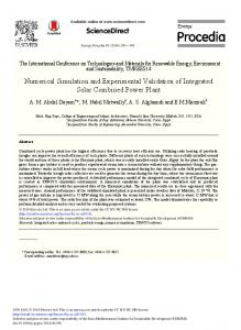
Representative plots of the optimized, deterministic point estimates for stress exponent(s) and critical stress(es) are plotted in Figs. 3 and 4 for G and C&G models, respectively. In these figures, the starting values are 3 and 3.3 for the glide and climb stress exponents, respectively. Other starting values between 1.8 and 4.2 for the G model and between 2.1 and 3.9 for the C&G model yield similar results, demonstrating that the optimized stress exponent(s), n are independent of temperature and strain-rate, and thus must be treated as calibration parameters. Furthermore, the optimization process indicates that bounds for the stress exponents can be restricted further (see the gray band on Figs. 3 and 4) from the ranges identified by the expert (recall Table 2). The further constrained ranges for the stress exponents are listed in Tables 3 and 4. On the other hand, the optimized critical stress, exhibit an exponential relationship with temperature and a linear relationship with strain-rate, which can be expressed as:
aebT
1 cedT 1 aebT 2 1
(16)
where is the strain-rate and T is the temperature. The variables a and c are the leading intercept coefficients for the exponential fit for the critical stress at a strain-rate of 1 0.001 and 2 1, respectively. Likewise, b and d are the decay rate coefficients for the exponential fit. In lieu of
17
ACCEPTED MANUSCRIPT
ACCEPTED MANUSCRIPT critical stresses, the coefficients a, b, c and d are treated as calibration parameters, for which posterior distributions are inferred. The optimal values for the coefficients computed from Eq. (12) and shown in Tables 3 and 4 for the two models, are treated as starting values during model calibration (discussed in the next section). The aforementioned analysis yields five calibration parameters for the G model and ten for
Downloaded by [Clemson University] at 19:01 25 November 2014
the C&G model as listed in Tables 3 and 4, along with the ranges, within which these parameters are allowed to vary to encompass available experimental data. Model Calibration Latin-hypercube designs with 140 and 240 samples are used to construct the GP emulators for the model predictions of the G model and the C&G model, respectively. For the calibration parameters, a uniform prior distribution is assumed between the ranges given in Tables 3 and 4. 10,000 accepted MCMC iterations are generated to estimate the posterior distribution of the calibration parameters. Exercising the GP emulators, predictions are obtained for 500 linearly spaced samples from the posterior distributions of the calibration parameters and GP hyperparameters. To compare the calibrated model predictions against experimental data, predictions, ( x , ) , are generated at experimental settings shown in Table 1.
RESULTS AND DISCUSSION This section demonstrates the resource allocation framework and provides a discussion on the computed systematic bias and information gain as the two versions of the VPSC model are calibrated using one through 11 available experiments in the sequence shown in Table 5. When all 11 experiments are used, coverage of the domain reaches over 85% according to the coverage metric proposed in Hemez et al. [17]. It is assumed that the minimum coverage threshold is set at
18
ACCEPTED MANUSCRIPT
ACCEPTED MANUSCRIPT 80% for this application, therefore the 11 experiments satisfactorily explore the domain of applicability. The calibrated VPSC models are executed to predict maximum stress along with texture 001 and 101 intensities at the settings of these 11 experiments. This section ultimately concludes by comparing the tradeoff of bias and uncertainty reduction between the two models through Divergence Information Criterion.
Downloaded by [Clemson University] at 19:01 25 November 2014
Initial Numerical Model: G model A reduction in uncertainty in the calibration parameters of the G model can be observed by the narrowing of the distributions in Fig. 5, which compares the posterior distributions of input parameters obtained using all 11 experiments to those obtained using only one experiment (with the exception of dg,, which can be explained by the relative insensitivity of this parameter). In Fig. 6, the stress and texture predictions depict convergent behavior with consistently reduced uncertainty as the number of experiments used in the analysis increases. Also evident in Fig. 6 is the constant systematic bias remaining after the convergence of predictions. The remaining systematic bias is measured to the nearest dashed horizontal line, which reflects the experimental uncertainty. Figs. 7(a)-9(a) depict the prediction bias for the maximum stress, texture 001, and texture 101 predictions at each experimental setting, as a function of the number of experiments used in the calibration process. For the maximum stress output shown in Fig. 7(a), little convergent behavior is evident; while for the texture outputs, upon addition of the fourth experiment, the inferred prediction bias of the textures converges for all prediction settings, as shown in Figs. 8(a) and 9(a).
19
ACCEPTED MANUSCRIPT
ACCEPTED MANUSCRIPT The information gain is also computed for the model predictions at all experimental settings (recall Table 5). For brevity, however, Fig. 10 shows the information gain plots for the maximum stress, texture 001, and texture 101 predictions at settings E and K, respectively. Remaining experimental settings show similar trends. For stress predictions, the information gain monotonically increases and ultimately converges. Slight fluctuations are expected given the
Downloaded by [Clemson University] at 19:01 25 November 2014
stochastic nature of the inference approach. For the texture predictions, a convergent behavior is not observed, indicating the G model’s inability to reproduce texture experiments at certain regions in the domain of applicability. Furthermore, Figs. 8-9 depict a prediction bias well in excess of 100% for the texture predictions demonstrating that uncertainty reduction alone is insufficient to warrant accurate predictions. In fact, Fig. 9 reveals a systematic bias for texture 101 over 400% for setting K, and as high as 1000% for setting J. Referring back to Fig. 1, the G model’s systematic bias is unacceptably high. The resource allocation framework then suggests that the rigor, in which the physics principles are modeled must be improved, which leads to the C&G model. Improved Numerical Model: C&G model In Fig. 11, it can be observed that the uncertainties in stress and texture predictions of the C&G model reduce and the prediction bias converges to a constant value as the number of experiments available for model calibration increases. Comparing Figs. 6 and 11, the more sophisticated, C&G model has significantly less prediction bias compared to the G model. However, the C&G model requires an increased number of experiments to reach convergence. For the C&G model, from Figs. 8 and 9, seven experiments are necessary for the prediction bias of the texture to converge; while convergence is achieved with only four experiments for the G
20
ACCEPTED MANUSCRIPT
ACCEPTED MANUSCRIPT model. An increased need for experiments to mitigate parameter uncertainty is expected for the C&G model, which has twice as many calibration parameters as the G model (see Tables 3 and 4). Fig. 12 shows the convergence of information gain after a sufficient number of experiments are used in the calibration process for experimental settings E and K. Note that since information
Downloaded by [Clemson University] at 19:01 25 November 2014
gain is calculated with respect to the initial uncertainty in input parameters, the specific level of information gain, at which convergence is achieved is irrelevant. The convergence of both the systematic bias and information gain indicates that prediction uncertainty is remedied. For the C&G model, the systematic bias converges to below 10% for the maximum stress prediction and below 50% for the texture predictions. Should this level of systematic bias be deemed acceptable for the intended purposes, the model may be considered validated, as the coverage exceeds the minimum coverage threshold. If additional reduction in systematic bias is required, however, a further physics sophistication of the model should be considered. A Comparative Analysis: Divergence Information Criterion In summary, according to the framework presented herein, the C&G is the preferred model for making predictions, as the G model is not validated. The lower converged discrepancy of the C&G model confirms that reduction in systematic bias can be achieved through physics sophistication of the code. However, note that due to increased complexity and a larger number of calibration parameters, the C&G model requires more experiments to reach convergence. Therefore, earlier discussion on the calibration of G and C&G models reveals a trade-off relationship between the prediction uncertainty and bias. Provided that both models are validated, preference of one model or the other can be reversed depending on the available
21
ACCEPTED MANUSCRIPT
ACCEPTED MANUSCRIPT experimental data. This section demonstrates this concept on the G and C&G models using the Divergence Information Criterion (DIC), a statistical metric for evaluating preferable models [31]. The DIC operates on the model input parameters and their distributions to create a metric that rewards a model for predicting closer to the experiments and penalizes a model for having a
Downloaded by [Clemson University] at 19:01 25 November 2014
larger effective number of parameters. The DIC is computed according to Eqs. (17)-(19).
p j 2 log[ f ( j ) ( y | ( j ) )] ( j ) ( ( j ) | y)d ( j ) 2 log[ f ( j ) ( y | ( j ) ( y))]
(17)
D j ( ( j ) ) 2 log[ f ( j ) ( y | ( j ) )] 2 log[ g ( j ) ( y )]
(18)
DIC D j (
( j)
) 2pj
(19)
In Eq. (17), p j is the proposed number of effective model parameters, f ( j ) ( y | ( j ) ) represents the probability density function for the experimental data y for a given for the j-th model, ( j ) represents the prior distribution of emulator parameters, and ( j ) ( y ) estimates ( j ) based upon the experimental data y [32]. In Eq. (18), 2log[ g ( j ) ( y )] is a standardizing term dependent on the observed data. In Eq. (19), p j represents p j when ( j ) ( y ) is equal to the posterior mean ( j ) . When comparing two models, a smaller value for DIC indicates a preferable model. As the DIC is used for comparison purposes only, the actual DIC values are only relevant relative to another model. Fig. 13 plots the DIC values computed for G and C&G models for increasing number of experiments. Until the fourth experiment, the less sophisticated G model has a lower DIC value and thus, the prediction bias outweighs the uncertainty in the parameters. If more than four
22
ACCEPTED MANUSCRIPT
ACCEPTED MANUSCRIPT experiments are available however, then the C&G model yields a smaller DIC value than that of the G model indicating that the lower prediction bias of the C&G model outweighs the penalty in higher prediction uncertainty due to a larger number of parameters. CONCLUSIONS It is a routine practice that numerical models are being validated against experiments
Downloaded by [Clemson University] at 19:01 25 November 2014
[33,34]. In this manuscript, we present a framework to guide the allocation of resources for the validation of numerical models. Improvement in the predictive capabilities of a numerical model can be achieved through the reduction of prediction uncertainty and bias. The prediction uncertainty can be reduced through calibration of model parameters against experimental data. An increase in the number of experiments used in the model calibration results in a decrease in prediction uncertainty, indicated by the convergence of the information gain to a stable level throughout the domain resulting in diminishing returns from additional experiments. In this case, improvements to predictive capabilities are only possible by reducing prediction bias, which can be achieved by improving the physics and/or engineering principles of the given model. The proposed framework is demonstrated on a non-trivial application of the VPSC code to predict stress and texture behavior of 5182 aluminum alloy. The availability of two versions of the VPSC code, G and C&G models, presents a unique opportunity to demonstrate the fundamental concepts behind the proposed resource allocation framework. In this example, for the G model, the systematic bias of the texture predictions converges, while the systematic bias of the stress predictions fails to converge as more experimental data is utilized in the calibration process. The analysis of the information gain shows that parameter uncertainty cannot be further reduced. As the prediction bias for stress fails to converge and the prediction bias for texture
23
ACCEPTED MANUSCRIPT
ACCEPTED MANUSCRIPT converges to an unacceptably high value, the C&G model, with an improved constitutive law, is employed. The convergence of the systematic bias and information gain of the C&G model is observed as the number of experiments available for model calibration increases. The prediction bias of the more sophisticated C&G model converges to a smaller value than that of the G model, but requires a higher number of experiments for convergence, demonstrating the trade-off
Downloaded by [Clemson University] at 19:01 25 November 2014
between reducing prediction bias and uncertainty in model validation. The logical thoughtprocess of the proposed framework can provide a science-based, quantifiable, and defendable rationale for allocating resources between code development and experimentation to reduce both uncertainty and bias in the predictions of complex numerical models. ACKNOWLEDGEMENTS This research is being performed using funding received from the DOE Office of Nuclear Energy's Nuclear Energy University Programs (Contract Number: 00101999). The editorial assistance of Godfrey Kimball of Clemson University is also acknowledged. Thanks to Karma Yonten, a former post-doctoral fellow at Clemson University for his assistance during the preparation of the manuscript.
24
ACCEPTED MANUSCRIPT
ACCEPTED MANUSCRIPT REFERENCES 1. M.A. Christie, J. Glimm, J.W. Grove, D.M. Higdon, D.H. Sharp, and M.M. Wood-Schultz, Error analysis and simulations of complex phenomena. Los Alamos Science, vol. 29, pp. 625, 2005. 2. T.G. Trucano, L.P. Swiler, T. Igusa, W.L. Oberkamp, and M. Pilch, Calibration, Validation,
Downloaded by [Clemson University] at 19:01 25 November 2014
and Sensitivity Analysis: What’s What, Reliability Engineering and System Safety, vol. 91, pp. 1331-1357, 2006. 3. S. Atamturktur, F. Hemez, B. Williams, C. Tome, and C. Unal, A forecasting metric for predictive modeling, Computers & Structures, vol. 98, pp. 2377-2387, 2011. 4. D. Draper, Assessment and Propagation of Model Uncertainty, Journal of the Royal Statistical Society, vol. 57, pp. 45-97, 1995. 5. D. Higdon, J. Gattiker, B. Williams, and M. Rightley, Computer model calibration using high-dimensional output, Journal of the American Statistical Association, vol. 103(482), pp. 570-583, 2008. 6. D. Higdon, C. Nakhleh, J. Gattiker, and B. Williams, A Bayesian calibration approach to the thermal problem, Computer Methods in Applied Mechanics and Engineering, vol. 197(2932), pp. 2431-2441, 2008. 7. M. Kennedy, and A. O’Hagan, Bayesian calibration of computer models (with discussion), Journal of the Royal Statistical Society Series B, vol. 68, pp. 425-464, 2001. 8. K. Van Buren, and S. Atamturktur, A Comparative Study: Predictive Modeling of Wind Turbine Blades, Journal of Wind Engineering, (accepted, in print).
25
ACCEPTED MANUSCRIPT
ACCEPTED MANUSCRIPT 9. I. Farajpour, and S. Atamturktur, Error and Uncertainty Analysis of Inexact and Imprecise Computer
Models,
ASCE
Journal
of
Computing
in
Civil
Engineering,
doi:
10.1061/(ASCE)CP.1943-5487.0000233, 2012. 10. J.E. Mottershead, and M.I. Friswell, Model Updating in Structural Dynamics: A Survey, Journal of Sound and Vibration, vol. 167(2), pp. 347-375, 1993.
Downloaded by [Clemson University] at 19:01 25 November 2014
11. F. Hemez, and J. Kamm, Computational Methods in Transport: Verification and Validation, Lecture Notes in Computational Science and Engineering, vol. 62 LNCSE, pp. 229-250, 2008. 12. M. Mollineaux, K. Van Buren, F. Hemez, and S. Atamturktur, Simulating the Dynamics of Wind Turbine Blades: Part I, Model Development and Verification, Wind Energy (accepted, in print), (Also, Los Alamos Report LA-UR-11-4996). 13. W.L. Oberkampf, T.G. Trucano, and C. Hirsch, Verification, validation, and predictive capability in computational engineering and physics, Sandia National Laboratories: Albuquerque, NM, SAND2003-3769, 2003. 14. B.H. Thacker, S.W. Doebling, F.M. Hemez, M.C. Anderson, J.E. Pepin, and E.A. Rodriguez, Concepts of model verification and validation, Los Alamos National Laboratories: Los Alamos, NM, LA-14167-MS, 2004. 15. D.E. Thompson, K.B. McAuley, and P.J McLellan, Design of optimal experiments to improve model predictions from a polyethelene molecular weight distribution model, Macromolecular Reaction Engineering, vol. 4(1), pp. 73-85, 2010. 16. M. Egeberg, and S. Atamturktur, Defining Coverage of a Domain with Validation Experiments Using a Modified Nearest-Neighbor Metric, Proceedings of 31th Society of
26
ACCEPTED MANUSCRIPT
ACCEPTED MANUSCRIPT Experimental Mechanics (SEM) International Modal Analysis Conference (IMAC-XXVIII), Orange County, California, USA, (to appear 2013). 17. F. Hemez,, S. Atamturktur, and C. Unal, Defining predictive maturity for validated numerical simulations, Computers and Structures Journal, vol. 88, pp. 497-505, 2010. 18. C.J. Stull, F. Hemez, B.J. Williams, C. Unal, and M.L. Rogers, An improved description of
Downloaded by [Clemson University] at 19:01 25 November 2014
predictive maturity for verification and validation activities, Los Alamos National Laboratories Technical Report, LA-UR-11-05659, 2011. 19. C.E. Shannon, A mathematical theory of communication, The Bell System Technical Journal, vol. 27, pp. 623-656, 1948. 20. W.K. Hastings, Monte Carlo sampling methods using Markov chains and their applications, Biometricka, vol. 57, pp. 97-109, 1970. 21. N. Metropolis, A.W. Rosenbluth, M.N. Rosenbluth, A.H. Teller, and E. Teller, Equations of State Calculations by Fast Computing Machines, Journal of Chemical Physics, vol. 21(6), pp. 1087-1092, 1953. 22. R.A. Lebensohn, and C.N. Tomé, A self-consistent anisotropic approach for the simulation of plastic deformation and texture development of polycrystals: application to zirconium alloys, Acta Materialia, vol. 41(9), pp. 2611-2623, 1993. 23. R.A. Lebensohn, Y. Liu, and P.P. Castañeda, On the accuracy of the self-consistent approximation for polycrystals: comparison with full-field numerical simulations, Acta Materialia, vol. 52, pp. 5347-5361, 2004.
27
ACCEPTED MANUSCRIPT
ACCEPTED MANUSCRIPT 24. R.A. Lebensohn, C.S. Hartley, C.N. Tomé, and O. Castelnau, Modeling the mechanical response of polycrystals deforming by climb and glide, Philosophical Magazine, vol. 90(5), pp. 567-583, 2010. 25. R.A. Lebensohn, R.A. Holt, J.A. Caro, A. Alankar, and C.N. Tomé, Improved constitutive description of single crystal viscoplastic deformation by dislocation climb, Comptes Rendus
Downloaded by [Clemson University] at 19:01 25 November 2014
Mecanique, vol. 340, pp. 289-295, 2012. 26. M.G. Stout, S.R. Chen, U.F. Kocks, A.J. Schwartz, S.R. MacEwen, and A.J. Beaudoin, Constitutive modeling of a 5182 aluminum as a function of strain rate and temperature, Hot Deformation of Aluminum Alloys II, Bieler T, Lalli TA, MacEwen LA, SR(Eds.), TMS: Warrendale, PA, USA, vol. 1009 pp. 205-216, 1998. 27. M.G. Stout, S.R. Chen, U.F. Kocks, A.J. Schwartz, S.R. MacEwen, and A.J. Beaudoin, Mechanisms responsible for texture development in a 5182 aluminum alloy deformed at elevated temperature, Hot Deformation of Aluminum Alloys II, Bieler T, Lalli TA, MacEwen LA, SR(Eds.), TMS: Warrendale, PA, vol. 1009, pp. 243-254, 1998. 28. M.J.D. Powell, A fast algorithm for nonlinearly constrained optimization calculations, Numerical Analysis, G.A. Watson (Eds.), Lecture Notes in Mathematics, Springer Verlag, vol. 630, 1978. 29. R.A. Waltz, J.L. Morales, J. Nocedal, and D. Orban, An interior algorithm for nonlinear optimization that combines line search and trust region steps, Mathematical Programming, vol. 107(3), pp. 391-408, 2006. 30. Nocedal, J. and S. J. Wright. Numerical Optimization, Second Edition. Springer Series in Operations Research, Springer Verlag, 2006.
28
ACCEPTED MANUSCRIPT
ACCEPTED MANUSCRIPT 31. D.J. Spiegelhalter, N.G. Best, B.P. Carlin, and A. van der Linde, Bayesian measure of model complexity and fit (with discussion), Journal of the Royal Statistical Society Series B, vol. 64, pp. 583-639, 2002. 32. B.J. Williams, R. Picard, L. Swiler, Multiple model inference with application to model selection for the reactor code R7, Los Alamos National Laboratories: Los Alamos, NM, LA-
Downloaded by [Clemson University] at 19:01 25 November 2014
UR-11-05625, 2011. 33. K. Li, X.-L. Gao, and A.K. Roy, Micromechanical Modeling of Viscoelastic Properties of Carbon Nanotube-Reinforced Polymer Composites, Mechanics of Advanced Materials and Structures, vol. 13(4), pp. 317-328, 2006. 34. A. El-Sabbagh, and A. Baz, A Coupled Nonlinear Model for Axisymmetric Acoustic Resonators Driven by Piezoelectric Bimorphs, Mechanics of Advanced Materials and Structures, vol. 13(2), pp. 205-217, 2006.
29
ACCEPTED MANUSCRIPT
ACCEPTED MANUSCRIPT
TABLES Table 1. Stress and texture intensity experimental results for 5182 Al
Temperature Experiment °
Downloaded by [Clemson University] at 19:01 25 November 2014
(C )
Stress
Texture
Texture
(MPa) @
Intensity
Intensity
Strain=0.6
(001)
(101)
Strain-Rate -1
(s )
A
200
10-3
226.2
1.00-1.41
4.00-6.00
B
300
10-3
91.4
0.58-0.71
4.00-6.00
C
350
10-3
50.0
2.00-2.83
2.83-4.00
D
400
10-3
30.6
NA
NA
E
500
10-3
14.9
4.00-6.00
2.00-2.83
F
550
10-3
7.0
NA
NA
G
200
1
280.0
NA
NA
H
300
1
193.7
NA
NA
I
400
1
121.3
1.41-2.00
4.00-6.00
J
500
1
65.5
2.00-2.83
0.00-0.58
K
550
1
43.0
2.83-4.00
0.58-0.71
30
ACCEPTED MANUSCRIPT
ACCEPTED MANUSCRIPT Table 2. Control and uncertain model parameter values Parameter
Minimum
Maximum
Control
Temperature (C°)
180
570
Parameters
Strain-Rate (s-1)
0.0005
1.05
ng
1
5
os (MPa)
1.2
1343.4
nc
1
5
os (MPa)
1.2
6045.4
Uncertain Downloaded by [Clemson University] at 19:01 25 November 2014
Model Parameters
Table 3. Calibration parameters for the G model Optimized/Mean Parameter
Min
Max
Value ag
4577.1
3432.8
5721.4
bg
-0.01
-0.008
-0.012
cg
372.48
279.36
465.60
dg
-0.005
-0.004
-0.006
ng
3.5
2.5
4.5
31
ACCEPTED MANUSCRIPT
ACCEPTED MANUSCRIPT
Table 4. Calibration parameters for the C&G model Optimized/Mean Parameter
Min
Max
Downloaded by [Clemson University] at 19:01 25 November 2014
Value ag
2970.2
2227.65
3712.75
bg
-0.008
-0.0064
-0.0096
cg
281.7
211.275
352.125
dg
-0.004
-0.0032
-0.0048
ng
3.5
2.5
4.5
ac
24727
18545.25
30908.75
bc
-0.012
-0.0096
-0.0144
cc
1595.2
1196.4
1994
dc
-0.008
-0.0064
-0.0096
nc
3.5
2.5
4.5
32
ACCEPTED MANUSCRIPT
ACCEPTED MANUSCRIPT
Downloaded by [Clemson University] at 19:01 25 November 2014
Table 5. Calibration experiments used in each case (see Table 1 for the experimental settings) Case
Experiments
1
A
2
A,B
3
A,B,C
4
A,B,C,E
5
A,B,C,E,I
6
A,B,C,E,I,J
7
A,B,C,E,I,J,K
8
A,B,C,E,I,J,K,D
9
A,B,C,E,I,J,K,D,E
10
A,B,C,E,I,J,K,D,E,G
11
A,B,C,E,I,J,K,D,E,G,H
33
ACCEPTED MANUSCRIPT
ACCEPTED MANUSCRIPT
LIST OF FIGURES
Downloaded by [Clemson University] at 19:01 25 November 2014
Fig.1. Predictive capability framework.
34
ACCEPTED MANUSCRIPT
ACCEPTED MANUSCRIPT
Downloaded by [Clemson University] at 19:01 25 November 2014
Fig.2. 5182 Al stress-strain curves for various temperatures and strain-rates.
Fig.3. Optimized point estimates for rate sensitivity (ng) (top) and critical stress (τ0) (bottom) for the G model.
35
ACCEPTED MANUSCRIPT
ACCEPTED MANUSCRIPT Fig.4. Optimized point estimates for rate sensitivities (ng and nc) (top) and critical stresses (τ0 and
Downloaded by [Clemson University] at 19:01 25 November 2014
σ0) (bottom) for the C&G model.
Fig.5. Posterior distribution for the G model (Left: one Experiment, Right: 11 Experiments) (Inner contour: 90th percentile, Outer contour: 50th percentile).
36
ACCEPTED MANUSCRIPT
ACCEPTED MANUSCRIPT Fig.6. Model prediction bias and uncertainty for the G model (Left: Experiment K, Right:
Downloaded by [Clemson University] at 19:01 25 November 2014
Experiment E).
37
ACCEPTED MANUSCRIPT
ACCEPTED MANUSCRIPT Fig.7. Systematic bias corresponding to maximum stress for each experiment: (a) G model, (b)
Downloaded by [Clemson University] at 19:01 25 November 2014
C&G model.
Fig.8. Systematic bias corresponding to texture 001 for each experiment: (a) G model, (b) C&G model.
38
ACCEPTED MANUSCRIPT
ACCEPTED MANUSCRIPT Fig.9. Systematic bias corresponding to texture 101 for each experiment: (a) G model, (b) C&G
Downloaded by [Clemson University] at 19:01 25 November 2014
model.
Fig.10. Information gain from experiments used for calibration of G model: (a) Experiment E, (b) Experiment K.
39
ACCEPTED MANUSCRIPT
ACCEPTED MANUSCRIPT Fig.11. Model prediction bias and uncertainty for the C&G model (Left: Experiment K, Right:
Downloaded by [Clemson University] at 19:01 25 November 2014
Experiment E).
40
ACCEPTED MANUSCRIPT
ACCEPTED MANUSCRIPT Fig.12. Information gain from experiments used for calibration of C&G model: (a) Experiment
Downloaded by [Clemson University] at 19:01 25 November 2014
E, (b) Experiment K.
Fig.13. DIC comparison of the G and C&G models with varying levels of experimental data.
41
ACCEPTED MANUSCRIPT