BASIN SCALE TSUNAMI PROPAGATION MODELING USING

WCCE – ECCE – TCCE Joint Conference: EARTHQUAKE & TSUNAMI

BASIN SCALE TSUNAMI PROPAGATION MODELING USING BOUSSINESQ MODELS: PARALLEL IMPLEMENTATION IN SPHERICAL COORDINATES J. T. Kirby1, N. Pophet2, F. Shi1, S. T. Grilli3 ABSTRACT We derive weakly nonlinear, weakly dispersive model equations for propagation of surface gravity waves in a shallow, homogeneous ocean of variable depth on the surface of a rotating sphere. A numerical scheme is developed based on the staggered-grid finite difference formulation of Shi et al (2001). The model is implemented using the domain decomposition technique in conjunction with the message passing interface (MPI). The efficiency tests show a nearly linear speedup on a Linux cluster. Relative importance of frequency dispersion and Coriolis force is evaluated in both the scaling analysis and the numerical simulation of an idealized case on a sphere. 1 INTRODUCTION The conventional models in the global-scale tsunami modeling are based on the shallow water equations and neglect frequency dispersion effects in wave propagation. Recent studies on tsunami modeling revealed that such tsunami models may not be satisfactory in predicting tsunamis caused by nonseismic sources (Løvholt et al., 2008). For seismic tsunamis, the frequency dispersion effects in the long distance propagation of tsunami fronts may become significant. The numerical simulations of the 2004 Indian Ocean tsunami by Glimsdal et al. (2006) and Grue et al. (2008) indicated the undular bores may evolve in shallow water, as the phenomenon evidenced in observations (Shuto, 1985). In the simulation for the same tsunami by Grilli et al. (2007), the dispersive effects were quantified by running the dispersive Boussinesq model FUNWAVE (Kirby et al., 1998) and the NSWE solver. Differences of up to 20% in surface elevations, between Boussinesq and NSWE simulations, were found in deeper water. Kulikov (2005) performed a wavelet frequency analysis based on satellite altimetry data recorded in the Bay of Bengal in deep water, and showed the importance of dispersive effects on wave evolution. He concluded that a long wave model including the dispersion mechanism should be used for this event. For global wave propagation, sphericity and Coriolis effects might play roles in simulating tsunami signals at far distant tide gauges. Dispersive Boussinesq models such as FUNWAVE are usually developed in Cartesian coordinates for modeling ocean wave transformation from intermediate water depths to the coast. Løvholt et al. (2008) recently reported a Boussinesq model including spherical coordinates and the Coriolis effect. The effects of the earth's rotation and the importance of Coriolis forces on the far-field propagation across the Atlantic Ocean were quantified in a model application to a potential tsunami from the La Palma Island. Although the Boussinesq models are believed to be more accurate tools than standard tsunami models (based on shallow water theory) in predicting dispersive tsunami waves, the efficiency of Boussinesq modeling of tsunamis is a concern. As pointed out by Yoon (2002), Boussinesq models consume huge computer resources due to the implicit nature of the solution technique used to deal with dispersion terms. Some simulations may involve a wide range of effects of interest, from propagation out of the generation region, through propagation at ocean basin scale, to runup and inundation at affected shorelines (Grilli et al., 2007). Approaches for improving model efficiency can be found in some practical applications such as using tested grids, unstructured or curvilinear grids (Shi et al., 2001) and the parallelization of computational codes (Sitanggang and Lynett, 2005). In this study, we derived weakly nonlinear, weakly dispersive model equations for surface gravity waves on the surface of a rotating sphere. A numerical model based on the equations was implemented using the domain decomposition technique in conjunction with the message passing interface (MPI). A numerical scheme is developed following the staggered-grid finite difference formulation of Shi et al. (2001). The efficiency of the model was examined in test cases with different number of computer processors. The relative importance of frequency dispersion and Coriolis force was evaluated in both the theory and the numerical simulation of an idealized case.

1

Center for Applied Coastal Research, University of Delaware Newark, USA, [email protected] Dept. Mathematics, Faculty of Science, Chulalongkorn Univ., Thailand 3 Department of Ocean Engineering University of Rhode Island, Narragansett, USA 2

1

WCCE – ECCE – TCCE Joint Conference: EARTHQUAKE & TSUNAMI

2 MODEL EQUATIONS IN SPHERICAL POLAR COORDINATES We consider motion in a fluid column of variable still water depth

r ′,θ , ϕ

where coordinates

z′ = r ′ − r

on the surface of a sphere,

denote radial distance from the sphere center, latitude, and longitude. We

denote the radius to the spherical rest surface as ′ 0

h′(ϕ ,θ )

r0′

and define a local vertical coordinate

z′

according to

. The dimensional Euler equations for incompressible inviscid flow are given by (Pedlosky 1979,

section 6.2)

2 w′

w′z′ + du ′

+

dt ′ dv′ dt ′

+

dw′

where

w′

r′ u′ r′

1 r′

+

1 r ′ cos θ

(v′ cos θ )θ +

1 r ′ cos θ

uϕ′ = 0

( w′ − v′ tan θ ) + 2Ω( w′ cos θ − v′ sin θ ) = −

(v′w′ + u ′2 tan θ ) + 2Ω sin θ u ′ = −

(u ′2 + v′2 )

ρ r′

1

ρ r ′ cos θ

pϕ′

pθ′

(2)

(3)

1

p′z ′ − g dt ′ r′ ρ u ′ and v′ are positive in the Easterly ( ϕ ) and Northerly ( θ −

− 2Ω cos θ u ′ = −

1

(1)

(4) ) directions respectively, and where

denotes vertical velocity. The total derivative operator is given by

d () dt ′

= ()t ′ +

u′ r ′ cos θ

()ϕ +

v′ r′

()θ + w′() z′

(5)

Boundary conditions consist of a dynamic condition specifying pressure

ps′ (ϕ , θ , t ′) = 0;

ps

z′ = η ′

on the water surface as (6)

together with kinematic constraints on the velocity field at the surface and bottom boundary. The kinematic surface boundary condition (KSBC) is given by

Dη ′ Dt ′

= w′;

z′ = η ′

(7)

and the bottom boundary condition (BBC) is given by

D(− h′) where

Dt ′ D() Dt ′

= w′;

= ()t +

z ′ = − h′

u′ r ′ cos θ

()ϕ +

(8)

v′ r′

()θ

(9)

Note that (8) allows for an imposed motion of the bottom to be incorporated. In Boussinesq or shallow water theory, it is typical to replace the local continuity equation (1) with a depthintegrated conservation equation for horizontal volume flux. Integrating (1) over depth and employing the kinematic boundary conditions (7) and (8) gives the exact equation

2

WCCE – ECCE – TCCE Joint Conference: EARTHQUAKE & TSUNAMI

(r )′2 |η ′ ηt′′ + (r )′2 |− h′ ht′′ +

{∫ cos θ ∂ϕ 1

∂

η′

}

u ′r ′dz ′ +

− h′

{∫ cos θ ∂θ 1

∂

η′

}

v′r ′dz ′ = 0

− h′

(10)

This will be simplified below based on scaling arguments. 2.1 Scaling Based on the usual notions for shallow water scaling, we introduce the length scales

h0′

,

a0′

and

λ′

to

denote a characteristic depth, a characteristic amplitude, and a characteristic horizontal length scale. Due to the close tie between source width and generated wave crest, λ ′ would normally be identified as a lengthscale

W

representing horizontal extent of the tsunami source region. Combinations of these scales

with each other and with

r0′

lead to a family of dimensionless parameters:

µ = h0′ / λ ′

relative depth or thickness of the ocean layer; dispersion in Boussinesq theory; and

ε

takes on values of

−3

O(10 )

δ =a /h ′ 0

′ 0

ε = h0′ / r0′

denoting the

, the usual parameter characterizing frequency

, the shallow water nonlinearity parameter. The parameter

at maximum, and will thus always be taken to indicate vanishingly small

effects when it occurs in isolation. Based on this family of parameters, we introduce dimensionless variables

( h, z ) =

We take

(h′, z ′) h0′

; η=

u0′ = δ c0′ = δ gh0′

η′

(11)

a0′ to denote a scale for horizontal velocities, and let

w0′

denote a scale for

vertical velocity, so that

(u, v) =

(u ′, v′) u0′

;

w=

w′

(12)

w0′

Pressure is scaled by the weight of the static reference water column,

p=

p′

(13)

ρ gh0′

We first introduce a rescaling of the dimensionless lattitude and longitude according to

(ϕ ∗ , θ ∗ ) =

r0′

λ′

(ϕ , θ ) =

µ ε

(ϕ , θ );

(14)

This gives horizontal coordinates which will change by

O(1)

amounts over the wavelength of a relatively

short wave. The nondimensional form of the continuity equation (1) is then given by (retaining terms to O(ε ) )

 w′  µ (1 − ε z ) [uϕ ∗ + (v cos θ )θ ∗ ] = O(ε 2 )  0  [ wz + 2ε w] + ′ u  cos θ  0 indicating that

w0′ = µu0′

(15)

, as is usual in a Boussinesq model framework. Turning to the depth-integrated

mass conservation equation (10), we introduce the total depth

H = h + δη

(16)

3

WCCE – ECCE – TCCE Joint Conference: EARTHQUAKE & TSUNAMI

and get

Ht + where

δ

( H u ) ∗ + ( H v cos θ ) ∗  = O(ε ) ϕ θ  cos θ 

(u, v) =

1 H

∫

δη −h

(u , v)dz

(18)

are depth averaged horizontal velocities, and where time

gh0′

t = ω ′t ′ =

λ′

(17)

t′

is scaled according to

t′

(19)

Equation (17) is the final volume flux conservation equation for the Boussinesq model system based on

(u , v) developed below. In keeping with the notion that waves which are short relative to the basin scale ′ ( λ ′ / r0 or ε / µ 1 ) may have frequencies which are high relative to the earth's rotation rate ε Ω′ ( ω ′ / Ω >> 1 ), we introduce the scaling Ω = ω (ϕ ) momentum ′ = O ( µ ) . Turning to the easterly equation (2), we obtain

ε  ut −   f (v − µ w tan θ ) + δ µ   where the Coriolis parameter

vt +

 u  δ −1 ε uϕ ∗ + vuθ ∗ + wu z − uv tan θ  + pϕ ∗ = O(ε )  µ  cos θ  cos θ

f = Ω sin θ

. The northerly

(θ )

momentum equation (3) becomes

 u  ε fu + δ  vϕ ∗ + vvθ ∗ + wvz + u 2 tan θ  + δ −1 pθ ∗ = O (ε ) µ µ  cos θ 

ε

The dimensionless

z



(21)

momentum equation is given by

  ε wϕ ∗ + vwθ ∗ + wwz  − fu cot θ  + ( pz + 1) = O (ε )  cos θ  µ2   u

δµ 2  wt + δ  

(20)

(22)

ε and µ ; the regime µ = O(ε ) , which recovers µ = O(ε 1/3 ) , which yields a Boussinesq approximation.

In the following, we consider two relations between the shallow water equations, and the regime 2.2 Shallow Water Equations

Most theories of transoceanic tsunami propagation are based on shallow water equations, in recognition of the vanishing effect of dispersion ( µ → 0) . In the present discussion, this limit is obtained in the limit of the horizontal lengthscale of wave motion approaching the horizontal scale of a global-sized ocean basin, or

λ ′ → r0′

. This implies that the ratio

ε / µ = O(1)

essentially the size of already neglected terms of

, while terms proportional to

O(ε )

µ

appearing alone are

. In this combined limit, the vertical momentum

equation (eq22) reduces to the hydrostatic balance, and may be integrated down from the free surface to yield

ph = δη − z

(23)

4

WCCE – ECCE – TCCE Joint Conference: EARTHQUAKE & TSUNAMI

where we subsequently use

ph

to denote the hydrostatic component of pressure. This expression is used to

evaluate pressure gradient terms in the horizontal momentum equations, yielding the final set of shallow water equations

1

Ht +

δ

1 cos θ

ut − f v +

( H u )ϕ + ( H v cos θ )θ  = 0  

1 cos θ

(24)

ηϕ = 0

(25)

v t + f u + ηθ = 0

(26)

where in this limit the scaled lattitude and longitude revert to the original values. Equation (24) retains the

ht

possibility of describing wave generation through a bottom motion effect

h′

since 2.3

is scaled by

′ 0

h

which appears at

O(1/ δ )

rather than wave amplitude.

The Boussinesq Approximation

We now wish to retain dispersive effects to leading order in the description of wave motion. Further, in order to provide a uniformly valid model which can be used to describe nonlinear wave evolution in shallow coastal margins as well as mainly linear evolution in the deep ocean basin, we will retain the mechanics of the fully nonlinear Boussinesq model framework, following largely the approach of Wei et al (1995) but working in the

(u , v)

framework of rotational flow. We will, for now, retain depth-averaged horizontal velocities

as

dependent variables rather than velocity at a reference elevation (as in Wei et al and subsequent efforts). In developing the model, we seek to retain terms to

O( µ 2 )

without any truncation in orders of

contrast to the classical Boussinesq approach, which would take

O(δ , δµ , µ ) 2

2

4

δ = O( µ ) 2

accompanied by the assumption that

µ = O(10 ) implies that

. This is in

and truncate terms of

and higher.

In the derivation, we will retain the effect of an imposed bottom motion −1

δ

µ = O(ε ) 1/3

. (For

ε = O(10 ) −3

h(t )

. The approximation is

, this implies a dispersion term

, which would be reasonable for the usual surface wave problem. This choice of scaling then

O(ε / µ ) = O( µ 2 )

, indicating that Coriolis terms and undifferentiated advective acceleration

terms are the same size as the leading order deviation from hydrostatic of the pressure term. 2.3.1

Pressure and vertical momentum

Pressure in the system being considered will deviate from hydrostatic by nonhydrostatic component by

p (ϕ ∗ ,θ ∗ , z , t ) =

p%

O( µ 2 )

amounts. Denoting this

, we write

ph (ϕ ∗ ,θ ∗ , z , t ) + δµ 2 p% (ϕ ∗ ,θ ∗ , z , t )

= δη − z + δµ 2 p%

(27)

Introducing (27 in (22) and integrating up to the free surface (where

p% = 0

δη δη  u  p% ( z ) = ∫ wt dz + δ ∫  wϕ ∗ + vwθ ∗ + wwz  dz + O (ε ) z z  cos θ 

The weakly nonlinear approximation with

δ / µ 2 = O(1)

5

would retain

) gives

(28)

WCCE – ECCE – TCCE Joint Conference: EARTHQUAKE & TSUNAMI

0

p% ( z ) = ∫ wt dz + O(δ )

(29)

z

2.3.2 The vertical structure of velocities In order to use (28) to evaluate horizontal pressure gradients, we need to establish a relation between and components u , v through the continuity equation (15), which simplifies to

wz +

µ  uϕ + (v cos θ )θ  = O(ε )   cos θ ∗

−h

Integrating (30) from

w( z ) = −

=−

2.3.3

z

(∫ cos θ ∂ϕ 1

∂

∗

1

(30)

∗

to

∂

cos θ ∂ϕ ∗

w

and using the bottom boundary condition gives z

)

uϕ ∗ dz −

−h

1

∂

cos θ ∂θ 1 ∂

∗

(∫

z

)

v cos θ dz −

−h

1

δ

ht

1

( u(h + z) ) − cosθ ∂θ ( v cosθ (h + z) ) − δ h + O(µ )

(31)

2

t

∗

Weakly nonlinear approximation

The standard Boussinesq approximation follows from the assumption that

δ = O( µ 2 )

.

To the required order, the perturbation to hydrostatic pressure is then given by

p% (ϕ ∗ , θ ∗ , z , t ) = where

BFT

2 (hu t ) ∗ + (h cos θ v t ) ∗  + z  ∗  ϕ θ  u ϕ t + (v cos θ )θ ∗t  + BFT cos θ  2 cos θ

z

(32)

denotes forcing terms resulting from motion of the ocean bottom,

1 ( z − δη )  (uht )ϕ ∗ + (v cos θ ht )θ ∗  BFT = − (δη − z )htt +  δ cos θ 

(33)

Using these results, the horizontal momentum equations are integrated over depth and the perturbation pressure is eliminated using the previous results. The final dimensionless equations are given by

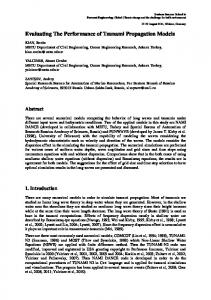
Figure 1: Relative importance of Coriolis force

(ε / µ ) and frequency dispersion ( µ 2 ) with varying inverse

source width

µ = h0 / W .

6

WCCE – ECCE – TCCE Joint Conference: EARTHQUAKE & TSUNAMI

1

δ

Ht +

1 cos θ

{( H u)

ϕ∗

}

+ ( H v cos θ )θ ∗ = 0

(34)

 u  1 ut − µ 2 f v + δ  uϕ ∗ + vuθ ∗  + ηϕ ∗ cos cos θ θ   2 2  µ h  ∗ ∗ h + uϕ ϕ t + (v cos θ )ϕ ∗θ ∗t  −  (hu t )ϕ ∗ϕ ∗ + (h cos θ vt )ϕ ∗θ ∗     2  cos 2 θ  6  

+

µ2 cos θ

(35)

( BFT )ϕ ∗ = O(δ 2 , δµ 2 , µ 4 )

 u  vt + µ 2 f u + δ  vϕ ∗ + vvθ ∗  + ηθ ∗  cos θ  2    h 1  h  1 +µ 2   uϕ ∗t + (v cos θ )θ ∗t  −  (hu t )ϕ ∗ + (h cos θ v t )θ ∗    6  cos θ θ ∗ 2  cos θ θ ∗  + µ 2 ( BFT )θ ∗ = O (δ 2 , δµ 2 , µ 4 )

{

2.3.4

{

}

}

Dispersion versus Coriolis

The orders of the frequency dispersions terms and Coriolis terms in Equations (35) and (36) are

O(ε / µ ) using

(36)

µ

2

respect to

O( µ 2 )

and

, respectively. The relative importance of frequency dispersion and Coriolis force can be evaluated and

µ

or

ε /µ h0 / W

values in some specific cases. Figure 1 illustrates variations of , where

W

100 km (2004 Indian Ocean tsunami),

µ2

and

ε /µ

represents width of tsunami source. Typically, for a source width of

µ ≈ 0.025

, the Coriolis effect is relatively much more important

than dispersion as shown in Figure 1. For a narrow source with a width of 25 km,

µ ≈ 0.1

, the dispersive

effect is as important as the Coriolis effect, and gets relatively more important as the source width diminishes. 3 NUMERICAL APPROACH Dimensional forms of equations (34) - (36) are discretized using the method described in Shi et al (2001). The system of equations is rewritten in a compact form as

Ht = E

(37)

U t = F (η , u , v) + F1 (v t ) + F2 (ht , ht t , u , v )

(38)

Vt = G (η , u , v) + G1 (u t ) + G2 (ht , ht t , u , v )

(39)

where

7

WCCE – ECCE – TCCE Joint Conference: EARTHQUAKE & TSUNAMI

E=−

1  ( H u )ϕ + ( H v cos θ )θ   r0 cos θ 

 h2  h 1 U =u+ 2 uϕϕ − (hu )ϕϕ   2 r0 cos θ  6 2  g 1 1 ηϕ F (η , u , v) = f v − uuϕ − vuθ − r0 cos θ r0 r0 cos θ  h2  h 1 (vt cos θ )ϕθ − (h cos θ v t )ϕθ   2 2 r0 cos θ  6 2  h h 1 h  F2 (ht , ht t , u , v) = − ( BFT )ϕ − 2 (ht u )ϕϕ + t (hu )ϕϕ  2  2 r0 cos θ 2r0 cos θ  2  F1 (v t ) = −

1  h2  1  h 1   (v cos θ )θ  −  (h cos θ v)θ   V =v+ 2   r0  6  cos θ θ 2  cos θ θ  1 1 g G (η , u , v) = − f u − uvϕ − vvθ − ηθ r0 cos θ r0 r0 1  h2  1  h 1   (hu t )ϕ   u tϕ  −  2   r0  6  cos θ θ 2  cos θ θ  h  1 1  h 1  (h cos θ v)θ  +  (ht cos θ v)θ  G2 (ht , ht t , u , v) = − ( BFT )θ + t  r0 2  cos θ θ 2  cos θ θ G1 (u t ) = −

In Equations (38) and (39), we introduce different properties.

F1

and

G1

F

and

G

F , F1 , F2 , G , G1

and

G2

to represent separately the terms with

include the Coriolis terms, pressure gradient terms and convective terms;

are the linear dispersive terms;

F2

and

G2

are the terms associated with motion of the

ocean bottom. The arrangement of cross-differentiated and time-derivative terms on RHS of Equations (Ut) and (Vt) makes the resulting set of LHS purely tridiagonal. A staggered grid in ϕ − θ plane is employed. The first-order spatial derivative terms are discretized to fourth-order accuracy by using five-point finite-differencing. The dispersive terms themselves are finite-differenced only to second-order accuracy, leading to error terms of

O(∆ϕ 2 , ∆θ 2 )

relative to the actual dispersive terms. In temporal discretization, the fourth-order Adams-

Bashforth-Moulton predictor-corrector scheme is employed. The corrector step is iterated until the error between two successive results reaches a required limit. 3.1

Parallelization

In parallelizing the computational model, we use the domain decomposition technique to subdivide the problem into multiple regions and assign each subdomain to a separate processor core. Each subdomain region contains an overlapping area of ghost cells two rows deep, as dictated by the 4th order computational stencil for the leading order non-dispersive terms. The Message Passing Interface (MPI) with non-blocking communication is used to exchange the data in the overlapping region between neighboring processors. Velocity components are obtained from Equation (41) and (42) by solving tridiagonal matrices using parallel pipelining tridiagonal solver described in Pophet et al (2008). To investigate performance of the parallel program, numerical simulations of the idealized ocean case are tested with different number of processors (8, 16, 24, 30 and 36 processors) of a linux cluster located at University of Delaware. The cluster has 8 computing nodes with 4 AMD Opteron 870 dual cores processors. Each node has 32 GBytes of main memory. The test case is set up in the computational domain of 90 o

o

o

90 E and 60 S - 60 N discretized into a 5401 generated using an Okada source.

8

×

o

W-

3601 numerical grid, and the initial wave is

WCCE – ECCE – TCCE Joint Conference: EARTHQUAKE & TSUNAMI

Figure 2: Variation in model performance with number of processors for a 5401 × 3601 domain. Straight line indicates arithmetic speedup. Actual performance shown by green line. Figure 2 shows the model speedup versus number of processors. It can be seen that a super linear speedup is obtained for the cases of 8 and 16 processors. This is due to the cache effect. When the size of sub-domain becomes small, the data set accessed frequently can fit into caches and the memory access time reduces dramatically. For the case with 24, 30 and 36 processors, speedup decreases and drops below linear speedup. This is due to the communication cost. The overlapping area increases with the number of processors. 4 AN OKADA SOURCE IN AN IDEALIZED OCEAN: SOURCE SIZE AND CORIOLIS EFFECTS To perform model tests with the spherical Boussinesq model, we generate a model grid in spherical coordinates and specify a flat bottom bathymetry in the ocean basin. The tsunami source is based on the standard half-plane solution for an elastic dislocation with maximum slip (Okada, 1985). Okada's solution is implemented in ''Tsunami open and progressive initial conditions system" (TOPICS) which provides the vertical co-seismic displacements as outputs. As an example, we specify a north-south oriented planar fault with centroid located at the equator. The tsunami source calculated by TOPICS is transferred and linearly superimposed into the sperical Boussinesq model, as an initial free surface condition as shown in Figure (3). Figure 4 demonstrates the evolution of tsunami wave front in time. The wave dispersion effect can be recognized by a train of waves near the wave front in cases with narrow tsunami sources. The Coriolis effect can be indicated by comparing model results with and without Coriolis force. Figure 5 shows the relative differences of surfave elevation between models with and without Coriolis force.

Figure 3: Source geometry for idealized tests of Coriolis and dispersion effects. Bottom displacement resulting from an Okada source aligned in North-South direction.

9

WCCE – ECCE – TCCE Joint Conference: EARTHQUAKE & TSUNAMI

Figure 4: Evolution of wave front in time in a constant depth ocean (t = 1, 2, 4, 6 hr). 5

CONCLUSIONS

In this study, weakly nonlinear, weakly dispersive model equations were derived for basin scale tsunami propagation on the surface of a rotating sphere . We introduce the scaling parameters representing respectively thickness of ocean layer, frequency dispersion in Boussinesq theory and shallow water nonlinearity for the Boussinesq approximation. The derivation followed the fully nonlinear Boussinesq model framework of We et al. (1995) but for rotational flow. The dispersive effects were retained as the leading order in the description of wave motion. A numerical scheme is developed based on the staggered-grid finite difference formulation of Shi et al (2001). The model is implemented using the domain decomposition technique in conjunction with the message passing interface (MPI). The efficiency tests show a nearly linear speedup on a Linux cluster. Relative importance of frequency dispersion and Coriolis force is evaluated in both the scaling analysis and the numerical simulation of an idealized case on a sphere.

Figure 5: Relative differences (%) of surface elevation between models with and without Coriolis force. Acknowledgements N. Pophet was supported by the Department of Civil and Environmental Engineering, University of Delaware, and by the Department of Ocean Engineering, University of Rhode Island. References Grue, J., Pelinovsky, E. N., Fructus, D., Talipova, T. and Kharif, C., 2008, ``Formation of undular bores and solitary waves in the Strait of Malacca caused by the 26 December 2004 Indian Ocean tsunami'', J. Geophys. Res., 113, C05008, doi:10.1029/2007JC004343.

10

WCCE – ECCE – TCCE Joint Conference: EARTHQUAKE & TSUNAMI

Glimsdal, S., G. Pedersen, K. Atakan, C. B. Harbitz, H. Langtangen, and F. Løvholt , 2006, ``Propagation of the Dec. 26, 2004 Indian Ocean tsunami: effects of dispersion and source characteristics'', Int. J. Fluid Mech. Res., 33(1), 15-43. Grilli, S. T., Ioualalen, M., Asavanant, J., Shi, F., Kirby, J. T. and Watts, P., 2007, ``Source constraints and model simulation of the December 26, 2004 Indian Ocean tsunami'', J. Waterway, Port, Coast. and Ocean Engrng., 133, 414-428. Imamura, F., N. Shuto, and C. Goto, 1988, ``Numerical simulation of the transoceanic propagation of tsunamis'', presented at Sixth Congress of the Asian and Pacific Regional Division, Int. Assoc. Hydraul. Res., Kyoto, Japan. Kirby, J. T., G. Wei, Q. Chen, A. B. Kennedy, and R. A. Dalrymple, 1998, ``Fully nonlinear Boussinesq wave model documentation and user's manual'', Research Rep. CACR-98-06, Center for Appl. Coastal Res., Univ. of Delaware, Newark. Kulikov, E., 2005, ``Dispersion of the Sumatra tsunami waves in the Indian Ocean detected by satellite altimetry.'' Rep. from P. P. Shirshov Institute of Oceanology, Russian Academy of Sciences, Moscow. Løvholt, F., Pedersen, G. and Gisler, G., 2008, ``Oceanic propagation of a potential tsunami from the La Palma Island'', J. Geophys. Res., 113, C09026, doi:10.1029/2007JC004603. Okada, Y., 1985, Surface deformtion due to shear and tensile faults in a half-space, Bull. Seismol. Soc. Am., 75(4), 1135-1154. Pedlosky, J., 1979, Geophysical Fluid Dynamics, Springer-Verlag, New York, pp.624. Pophet, N., 2008, ``Parallel computation for tsunami'', M.S. Thesis, Chulalongkorn University Pophet, N., Kaewbanjak, N., Asavanant, J. and Ioualalen, M., 2008, ``Parallelization of fully nonlinear Boussinesq equations for tsunami simulations: new approach on higher grid resolution for tsunami simulation using parallelized fully nonlinear Boussinesq Equations'', submitted to Computer and Fluids. Shi, F., Dalrymple, R. A., Kirby, J. T., Chen, Q. and Kennedy, A., 2001, ``A fully nonlinear Boussinesq model in generalized curvilinear coordinates'', Coastal Engrng., 42, 337-358. Shuto, N., 1985, ``The Nihonkai-Chubu earthquake tsunami on the north Akita Coast", Coastal Eng. Jpn., 28, 255-264. Sitanggang, K. and Lynett, P. , 2005, ``Parallel computation of a highly nonlinear Boussinesq equation model through domain decomposition'', International Journal for Numerical Methods in Fluids, 49, 57-74. Tappin, D. R., Watts, P. and Grilli, S. T., 2008, ``The Papua New Guinea tsunami of 17 July 1998: anatomy of a catastrophic event'', Nat. Hazards Earth Syst. Sci., 8, 243-266. Wei, G., Kirby, J. T., Grilli, S. T. and Subramanya, R., 1995, ``A fully nonlinear Boussinesq model for surface waves. I. Highly nonlinear, unsteady waves'', J. Fluid Mech., 294, 71-92. Yoon, S. B., 2002, ``Propagation of distant tsunamis over slowly varying topography'', J. Geophys. Res., 107(C10), 3140, doi:10.1029/2001JC000791.

11