BATCH SCHEDULING IN A TWO-STAGE FLEXIBLE ...

FOUNDATIONS Vol. 39

OF

COMPUTING AND (2014)

DECISION

DOI: 10.2478/fcds-2014-0001

SCIENCES No. 1

ISSN 0867-6356 e-ISSN 2300-3405

BATCH SCHEDULING IN A TWO-STAGE FLEXIBLE FLOW SHOP PROBLEM Enrique Gerstl*, Gur Mosheiov * and Assaf Sarig**

Abstract. We study a special two-stage flexible flowshop, which consists of several parallel identical machines in the first stage and a single machine in the second stage. We assume identical jobs, and the option of batching, with a required setup time prior to the processing of a new batch. We also consider the option to use only a subset of the available machines. The objective is minimum makespan. A unique optimal solution is introduced, containing the optimal number of machines to be used, the sequence of batch sizes, and the batch schedule. The running time of our proposed solution algorithm is independent of the number of jobs, and linear in the number of machines. Keywords: Deterministic Scheduling, Flexible Flowshop, Batch Scheduling

1.

Introduction

A flexible flowshop is a machine setting consisting of several stages in series, where each stage contains a number of parallel machines. Minimizing makespan on a general flexible flowshop is clearly NP-hard, since it is a generalization of both minimum makespan on parallel identical machines and minimum makespan on a classical flowshop (with at least three machines). In fact, minimum makespan on a flexible flowshop was shown to be strongly NP-hard even for the special case of (𝑖𝑖) two stages, (𝑖𝑖𝑖𝑖) two identical machines in one stage and a single machine in the second stage, and (𝑖𝑖𝑖𝑖𝑖𝑖) when preemption is allowed (Hoogeveen et al. [11]). We refer the reader to the recent survey on flexible flowshops by * Enrique Gerstl, School of Business Administration, The Hebrew University, Jerusalem, Israel; Gur Mosheiov, School of Business Administration, The Hebrew University, Jerusalem, Israel. ** Assaf Sarig, The Center for Academics Studies, Or Yehuda, Israel Acknowledgement: This paper was supported in part by The Recanati Fund and The Charles Rosen Chair of Management, The School of Business Administration, The Hebrew University, Jerusalem, Israel.

Unauthenticated Download Date | 11/24/15 6:03 AM

4

E. Gerstl, G. Mosheiov, A. Sarig

Ruiz and Vazquez-Rodriguez [25], which contains 225 references, dealing with various combinations of flexible flowshop settings and objective functions. Several researchers studied the special two-stage flexible flowshop setting, where the first stage consists of 𝑚𝑚 parallel identical machines and the second stage contains a single machine. This setting is known in the literature as look-behind flowshop (LBFS); see e.g., Lee and Vairaktarakis [15]. LFBS has numerous applications, including the standard manufacturing system of several parallel identical production machines followed by a single machine (station) for painting, rapping, loading, assembly, etc. [Lee and Vairaktarakis [15] also defined the symmetric setting, in which the first stage contains a single machine and the second stage consists of 𝑚𝑚 parallel identical machines. They denoted this setting by LAFS (look-ahead flexible flowshop).] A similar setting of a twostage flowshop with a single (critical) machine in one of these stages and several dedicated machines in the other stage has been studied by e.g., Oguz et al. [23], Cheng and Kovalyov [5], Lin [16], Kyparisis and Koulamas [14], Lin and Liao [17], Mosheiov and Yovel [21], Cheng et al. [6], Oguz and Ercan [22], and Gerstl and Mosheiov [9], among others. In this paper we focus on an LFBS system, in the context of batch scheduling; see e.g., Monma and Potts [18] and Allahverdi et al. [1]. Recall that in batch scheduling jobs may be grouped and processed in batches. The processing time of a batch is identical to the total processing times of the jobs contained in the batch. Prior to starting a new batch (either on one of the first stage machines, or on the second stage machine), a setup time is performed, during which the production process is stopped. Each of the batches is performed on one of the first stage machines, and upon completion, continues (as a batch) to the second stage machine. Each first-stage machine can process (at most) a single batch. As commonly assumed in batch scheduling models, we consider: (𝑖𝑖) batch availability, i.e., jobs can start processing on the second-stage machine only when their entire batch is completed on the first-stage machine; (𝑖𝑖𝑖𝑖) non-anticipatory setup times, i.e., prior to starting the batch setup on the second-stage machine, the entire batch must be completed and released from the first-stage machine; (𝑖𝑖𝑖𝑖𝑖𝑖) batch consistency, i.e., a batch remains unchanged on the firststage and on the second-stage machine. Finally, we consider here the very practical setting of identical processing time jobs. The numerous studies of scheduling identical jobs reflect the many applications of this setting, in particular the many types of production lines of identical items (see e.g., the two recent surveys: Baptiste and Brucker [2], and Kravchenko and Werner [13]). We note that the special case of the problem studied here; where the parallel machines in each stage of the flexible flowshop are replaced by a single machine (i.e., minimizing makespan on an 𝑚𝑚-machine flowshop with identical jobs and batching) has been solved in Mosheiov and Oron [19]. In a recent paper, Fanjul-Peyro and Ruiz [7] introduced and tested numerically algorithms for solving systems with the option of using only a subset of all the available machines. They focused on the option of Not-All-Machines (NAM) on parallel-unrelated machines. Previously, Cao et al. [3] introduced a tabu search algorithm to minimize the machine holding cost for a NAM model on parallel identical machines; Chen and Li [4] considered the case that the number of machines can be reduced by outsourcing jobs to an external production line; Finke et al. [8] studied a NAM model with precedence constraints, and Kravchenko and Werner [12] considered NAM problems with release dates and deadlines. Among the many applications of the NAM decision, Fanjul-Peyro and Ruiz [7] mention a typical setting of a shop in which some machines remain idle due to the large capacity of the system, which exceeds the total demand.

Unauthenticated Download Date | 11/24/15 6:03 AM

Batch scheduling in a two-stage flexible flow shop problem

5

Given all the above (unit jobs, batching, NAM), an optimal solution for our proposed LBFS model consists of the following decisions: (i) How many first-stage machines to use; (ii) Given the number of machines - how to allocate jobs to batches; and (iii) How to schedule these batches. First we introduce a lower bound on the optimal makespan, obtained by solving to optimality the relaxed version of the problem in which non-integer batch sizes are permitted. This solution consists of a unique increasing sequence of batch sizes. Then, we convert this solution into an optimal integer schedule. The total running time is shown to be independent of the number of jobs, and is linear in the number of firststage machines. (As indicated later, the running time of the algorithm is not polynomial in the input size. However, since the number of batches that need to be calculated and stored is of the order of the number of the machines, this running time seems to be the smallest possible.) In a recent paper, Gerstl and Mosheiov [10] studied the LAFS version of the problem, i.e., when a single machine is considered in stage 1, and 𝑚𝑚 parallel identical machines in stage 2. LAFS and LBFS may have significantly different applications. An LAFS system may consist of a single common production machine followed by several parallel customization stations. LBFS may model a plant having a number of parallel manufacturing units in stage one, followed by e.g., a common quality-control/rapping/painting station. Despite the different nature of the two models, the analysis of both appears to be related. Using a similar approach to that used by Gerstl and Mosheiov [10], we obtain a nonstandard sequence of optimal batch sizes for the relaxed version of the problem (where noninteger batch sizes are allowed). We then introduce a rounding procedure, which guarantees an optimal solution for the original (integer) version. The paper is organized as follows: Section 2 contains the notation and the problem formulation; Section 3 provides the lower bound based on the solution of the relaxed version; Section 4 presents the optimal integer solution.

2.

Formulation

We study a 2-stage flexible flowshop (𝐹𝐹𝐹𝐹𝐹𝐹), where the first stage consists of 𝑚𝑚 parallel identical machines, and the second stage consists of a single common machine (called critical). We denote this special flowshop structure by 𝐹𝐹𝐹𝐹𝑠𝑠(𝑚𝑚, 1). There are 𝑛𝑛 identical jobs, which are assumed to have unit processing times after appropriate scaling. Thus, if 𝑝𝑝!" denotes the processing time of job 𝑗𝑗 on machine 𝑖𝑖, we have 𝑝𝑝!" = 1, 𝑖𝑖 = 1, … , 𝑚𝑚 + 1, 𝑗𝑗 = 1, … , 𝑛𝑛 (where machine 𝑚𝑚 + 1 is the critical machine). The jobs processed on machine 𝑖𝑖  (𝑖𝑖 = 1, . . . , 𝑚𝑚)  are processed later as a single block (batch) on the critical machine. An integer setup time, denoted by 𝑆𝑆, is required prior to starting the process of a batch on each of the first 𝑚𝑚 machines, as well as on the critical machine. We assume a machineindependent setup time. If 𝑘𝑘 machines are used in the first stage (𝑘𝑘 ≤ 𝑚𝑚), then for a given allocation of jobs to these 𝑘𝑘 machines, the number of jobs assigned to machine 𝑖𝑖 is denoted ! by 𝑛𝑛! , 𝑖𝑖 = 1, … , 𝑘𝑘. Clearly, !!! 𝑛𝑛! = 𝑛𝑛 . Finally, recall that our model assumes batch availability, non-anticipatory setup times, and batch consistency; see above. For a given schedule, the completion time of the last job on machine 𝑖𝑖 (i.e., the completion time of batch 𝑖𝑖 on the first stage machine) is denoted by 𝐶𝐶! , 𝑖𝑖 = 1, … , 𝑘𝑘. The

Unauthenticated Download Date | 11/24/15 6:03 AM

6

E. Gerstl, G. Mosheiov, A. Sarig

(!")

completion time of batch 𝑖𝑖 on the critical machine is denoted by 𝐶𝐶! !"

𝐶𝐶!"# = max  {𝐶𝐶! , 𝑖𝑖 = 1, … , 𝑘𝑘}. 𝐹𝐹𝐹𝐹𝐹𝐹(𝑚𝑚, 1)/  𝑆𝑆, 𝑝𝑝!" = 1  /𝐶𝐶!"# .

3.

, 𝑖𝑖 = 1, … , 𝑘𝑘. Let

Thus, the problem studied in this paper is:

A lower bound on the optimal makespan value

A solution for the problem 𝐹𝐹𝐹𝐹𝐹𝐹(𝑚𝑚, 1)/  𝑆𝑆, 𝑝𝑝!" = 1  /𝐶𝐶!"# consists of: (𝑖𝑖) a decision on the optimal number of (the first-stage) machines to be used, (𝑖𝑖𝑖𝑖) the allocation of jobs to machines, and (𝑖𝑖𝑖𝑖𝑖𝑖) the job schedule. According to the well-known reversibility property in flowshops, the makespan does not change if the jobs go through the flowshop in the opposite direction in the reverse order; see e.g. Pinedo [24]. Thus, a possible solution procedure could be based on the reversed solution of 𝐹𝐹𝐹𝐹𝐹𝐹(1, 𝑚𝑚)/  𝑆𝑆, 𝑝𝑝!" = 1  /𝐶𝐶!"# , given in (10). However, due to the different structure of the optimal schedules in both cases, we introduce in the following the properties of an optimal schedule for 𝐹𝐹𝐹𝐹𝐹𝐹(𝑚𝑚, 1), and consequently we provide a complete solution for this problem. We first solve the relaxed version of the problem, allowing non-integer batch sizes. The optimal solution for the relaxed version is clearly a lower bound on the optimal makespan of 𝐹𝐹𝐹𝐹𝐹𝐹(𝑚𝑚, 1)/  𝑆𝑆, 𝑝𝑝!" = 1  /𝐶𝐶!"# . We use the following notation for the relaxed version: (!)

𝑛𝑛!

(!)

is the size of batch 𝑖𝑖 in the relaxed version, 𝐶𝐶! is the completion time of batch 𝑖𝑖 on (!",!)

the first stage machine, and 𝐶𝐶! (∗,!) 𝐶𝐶!"#

is the completion time of batch 𝑖𝑖 on the critical

is the optimal makespan for the relaxed version. In the following we prove machine. several properties of an optimal schedule: Property 1: If 𝑆𝑆 ≥ 𝑛𝑛, an optimal schedule exists such that a single machine is used in the first stage (𝑘𝑘 = 1).

Proof: For 𝑘𝑘 = 1 (single machine is used in the first stage) the makespan is 2𝑆𝑆 + 2𝑛𝑛. For ∎ 𝑘𝑘 ≥ 2 the makespan is at least 𝑘𝑘 + 1 𝑆𝑆 + 𝑛𝑛, which is larger than 2𝑆𝑆 + 2𝑛𝑛. In the remainder of this paper we assume 𝑆𝑆 < 𝑛𝑛.

Property 2: For a given number 𝑘𝑘 of machines used, an optimal schedule exists such that (!) (!) 𝑛𝑛!!! = 𝑆𝑆 + 2𝑛𝑛! , 𝑖𝑖 = 1, … , 𝑘𝑘 − 1. (!)

(!)

Proof: We focus first on the first two batches, and prove that 𝑛𝑛! = 𝑆𝑆 + 2𝑛𝑛! . (!) (!) Assume that an optimal schedule 𝑞𝑞 exists such that: 𝑛𝑛! > 𝑆𝑆 + 2𝑛𝑛! . The completion (!) !",! (𝑞𝑞) = 2𝑆𝑆 + 2𝑛𝑛! . Let time of the second batch on the critical machine is given by: 𝐶𝐶! (!) (!) (!) 𝜖𝜖 = 𝑛𝑛! − 𝑆𝑆 − 2𝑛𝑛! > 0. We create a schedule 𝑞𝑞′ by increasing 𝑛𝑛! by 𝜖𝜖/3 (𝑛𝑛!′ = (!) (!) (!) !",! 𝑞𝑞 ′ = 𝑛𝑛! + 𝜖𝜖/3), and decreasing 𝑛𝑛! by 𝜖𝜖/3 (𝑛𝑛!′ = 𝑛𝑛! − 𝜖𝜖/3). We obtain: 𝐶𝐶! (!) !" 2𝑆𝑆 + 2𝑛𝑛!′ = 2𝑆𝑆 + 2(𝑛𝑛! − 𝜖𝜖/3) < 𝐶𝐶! (𝑞𝑞).

Unauthenticated Download Date | 11/24/15 6:03 AM

Batch scheduling in a two-stage flexible flow shop problem

(!)

7

(!)

Assume now that in schedule 𝑞𝑞: 𝑛𝑛! < 𝑆𝑆 + 2𝑛𝑛! . The completion time of the second (!) (!) (!) !",! 𝑞𝑞 = 3𝑆𝑆 + 2𝑛𝑛! + 𝑛𝑛! . Let 𝜖𝜖 = 2𝑛𝑛! + batch on the critical machine is given by: 𝐶𝐶! (!) (!) (!) 𝑆𝑆 − 𝑛𝑛! > 0. We create a schedule 𝑞𝑞′ by decreasing 𝑛𝑛! by 𝜖𝜖/3 (𝑛𝑛!′ = 𝑛𝑛! − 𝜖𝜖/3), and (!) (!) !",! 𝑞𝑞 ′ = 3𝑆𝑆 + 2𝑛𝑛!′ +   𝑛𝑛!′ = increasing 𝑛𝑛! by 𝜖𝜖/3 (𝑛𝑛!′ = 𝑛𝑛! + 𝜖𝜖/3). We obtain: 𝐶𝐶! (!) (!) !",! (𝑞𝑞). 3𝑆𝑆 + 2(𝑛𝑛! − 𝜖𝜖/3) + (𝑛𝑛! + 𝜖𝜖/3) < 𝐶𝐶! (!) (!) We conclude that schedule 𝑞𝑞′ (with 𝑛𝑛! = 𝑆𝑆 + 2𝑛𝑛! ) is optimal as well. (!) (!) The remaining proof is by induction. Assume that 𝑛𝑛!!! = 𝑆𝑆 + 2𝑛𝑛! , 𝑖𝑖 = 1, … , 𝑙𝑙 for (!) (!) some 𝑙𝑙 < 𝑘𝑘 − 1. A similar proof leads to the equality 𝑛𝑛!!! = 𝑆𝑆 + 2𝑛𝑛!!! . It follows that for (!)

(!)

a given 𝑘𝑘 values, 𝑛𝑛!!! = 𝑆𝑆 + 2𝑛𝑛! , 𝑖𝑖 = 1, … , 𝑘𝑘 − 1.

∎

Property 3: For a given number 𝑘𝑘 of machines used, an optimal schedule exists such that (!)

(!)

𝑛𝑛!

(!)

=

!!!(!! !!!!) !! !!

(1)

(!)

Proof: Since 𝑛𝑛!!! = 𝑆𝑆 + 2𝑛𝑛! , 𝑖𝑖 = 1, … , 𝑘𝑘 − 1 (Property 2), we can easily express 𝑛𝑛! as a (!) function of 𝑛𝑛! and 𝑆𝑆: From

(!) 𝑛𝑛! + (!) 𝑛𝑛! ).

(!) ! = !!! 𝑛𝑛! (!) ! !!! 2𝑛𝑛!!! + 𝑆𝑆

Thus,

(!)

(!)

𝑛𝑛! = 2!!! 𝑛𝑛! + 2!!! − 1 𝑆𝑆.

𝑛𝑛 and Property 2, it follows: 𝑛𝑛 = =

(!) 𝑛𝑛!

!!! (!) !!! 𝑛𝑛!

+ 𝑘𝑘 − 1 𝑆𝑆 + 2 (!)

𝑛𝑛! =

(!)

!!!! ! !!! ! !

=

(2)

(!) ! !!! 𝑛𝑛! (!) 𝑛𝑛! +

(!)

= 𝑛𝑛! +

𝑘𝑘 − 1 𝑆𝑆 + 2(𝑛𝑛 −

.

(!)

=

(!)

!!! !! !!!! !! !!

=

(3)

From equations (2) and (3) we obtain that 2!!! 𝑛𝑛! + 2!!! − 1 𝑆𝑆 = follows that: 𝑛𝑛!

(!) ! !!! 𝑛𝑛!

(!)

!!!! ! !!! !

.

!

(4)

. It ∎

Based on Properties 2 and 3, the makespan value for a given 𝑘𝑘 value is the sum of the idle time on the critical machine (which is identical to the setup time and the total (!) processing time of the first batch, i.e., 𝑆𝑆 + 𝑛𝑛! ), and the total processing time of the 𝑘𝑘 batches on the critical machine (i.e., 𝑘𝑘𝑘𝑘 + 𝑛𝑛). Thus, (!",!)

𝐶𝐶!

(!)

= 𝑆𝑆 + 𝑛𝑛! + 𝑘𝑘𝑘𝑘 + 𝑛𝑛 = 𝑆𝑆 𝑘𝑘 + 1 +

!!!(!! !!!!) !! !!

+ 𝑛𝑛.

(5)

In order to find the optimal makespan value (for the relaxed version), we have to solve (5) for all 𝑘𝑘 values. Let 𝑘𝑘 ∗ denote the optimal number of machines used. Clearly, 1 ≤ 𝑘𝑘 ∗ ≤ 𝑚𝑚. The following property introduces better bounds on 𝑘𝑘 ∗ : Property 4: The optimal number of machines to be used is bounded by:

Unauthenticated Download Date | 11/24/15 6:03 AM

8

E. Gerstl, G. Mosheiov, A. Sarig

𝑙𝑙𝑙𝑙𝑙𝑙! 1 +  

! !

+ 1 𝑙𝑙𝑙𝑙 2

≤ 𝑘𝑘 ∗ ≤ 𝑙𝑙𝑙𝑙𝑙𝑙! 1 +  

(!",!)

! !

+ 𝑚𝑚 𝑙𝑙𝑙𝑙 2 .

(6)

Proof: Allowing 𝑘𝑘 to be non-integer, 𝐶𝐶! is continuous and convex in 𝑘𝑘. Thus, the optimal (non-integer) 𝑘𝑘 value can be found by standard derivation. The derivative of (5) with respect to 𝑘𝑘 is: (!",!)

!!!

(!",!)

!!!

!"

!"

= 𝑆𝑆 +

!!!! !" ! !! !! !! ! !!! !! !!!! !! !" ! !! !!

!

= 0 leads to: 𝑆𝑆2! − 𝑆𝑆𝑆𝑆 ln 2 = 𝑆𝑆 + 𝑛𝑛 ln 2 , or 2! − 𝑘𝑘 𝑙𝑙𝑙𝑙 2 = 1 +

! !" ! !

.

.

(7)

Since 1 ≤ 𝑘𝑘 ≤ 𝑚𝑚, the left-hand-side of (7) is bounded by: It follows that:

2! − 𝑚𝑚 ln 2 ≤ 2! − 𝑘𝑘 ln 2 ≤ 2! − ln 2 . 2! − 𝑚𝑚 ln 2 ≤ 1 +

! !" ! !

≤ 2! − ln 2 .

We obtain the following bounds on the optimal number of machines used: 𝑘𝑘 ∗ ≤ log ! 1 +  

𝑘𝑘 ∗ ≥ log ! 1 +  

! !

! !

+ 𝑚𝑚 ln 2 ; + 1 ln 2 .

Since 𝑘𝑘 is clearly bounded by 𝑚𝑚, and must be an integer, the actual upper bound on its value is

∎

𝑘𝑘 !" ≡ min   𝑚𝑚, log ! 1 +  

!

+ 𝑚𝑚 ln 2

.

(8)

𝑘𝑘 !" ≡ 𝑚𝑚𝑚𝑚𝑚𝑚   𝑚𝑚, log ! 1 +  

!

+ 1 ln 2

.

(9)

Similarly, the actual lower bound on 𝑘𝑘 is

!

!

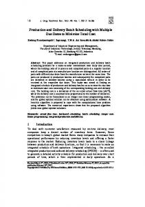
The optimal number of machines, 𝑘𝑘 ∗ , is a non-decreasing function of the number of jobs 𝑛𝑛, and a non-increasing function of the setup time 𝑆𝑆. Figure 1 demonstrates 𝑘𝑘 ∗ as a function of 𝑛𝑛 (for a given 𝑆𝑆 value; 𝑆𝑆 = 20). Similarly, Figure 2 demonstrates 𝑘𝑘 ∗ as a function of 𝑆𝑆 (for a given 𝑛𝑛 value; 𝑛𝑛 = 1000).

Unauthenticated Download Date | 11/24/15 6:03 AM

Batch scheduling in a two-stage flexible flow shop problem

9

7  

k*  

6  

5   4   3   2   1   0  

Figure 1.

0  

500  

1000  

n  

1500  

2000  

2500  

The optimal number of used machines as a function of the number of jobs (𝑺𝑺 = 𝟐𝟐𝟐𝟐).

k*  

10   8   6  

4   2   0  

Figure 2.

0  

200  

400  

S  

600  

800  

1000  

The optimal number of used machines as a function of the setup time (𝒏𝒏 = 𝟏𝟏𝟎𝟎𝟎𝟎𝟎𝟎).

Based on all the above, we introduce in the following a formal algorithm: Lower Bound Algorithm (optimum of the relaxed version): Input: 𝑚𝑚, 𝑛𝑛, 𝑆𝑆; Step 1: Calculate 𝑘𝑘 !" and 𝑘𝑘 !" from (8) and (9). Step 2: For 𝑘𝑘 = 𝑘𝑘 !" to 𝑘𝑘 !" (!",!) Calculate 𝐶𝐶! from (5). (∗,!)

(!",!)

Step 3: The optimal makespan is given by (5): 𝐶𝐶!"# = min! !" !!!! !" 𝐶𝐶! 𝑘𝑘 ∗ is the appropriate 𝑘𝑘 value.

Unauthenticated Download Date | 11/24/15 6:03 AM

.

10

E. Gerstl, G. Mosheiov, A. Sarig

The optimal sequence of batch sizes is given by (4) and (2) (for 𝑘𝑘 ∗ ).

Running Time: Step 1 requires a constant time. Step 2 is performed 𝑂𝑂(𝑚𝑚) times, and each (∗,!) iteration requires a constant time. Finding 𝐶𝐶!"# in Step 3 requires 𝑂𝑂(𝑚𝑚), and then calculating the batch sizes requires 𝑂𝑂(𝑚𝑚) as well. Thus, the total running time is 𝑂𝑂(m).

Numerical Examples: In the following we provide the solution for three 20-machine problems. The problems are different significantly from each other in the ratio 𝑛𝑛/𝑆𝑆. As expected (see (8) and (9)), the number of candidates for the optimal number of machines decreases as this ratio increases. Example 1: 𝑛𝑛 = 1,000, 𝑆𝑆 = 8, 𝑚𝑚 = 20. In Step 1 of the algorithm we calculate the following bounds: 𝑘𝑘 !" = 6.665;  𝑘𝑘 !" = 6.465. It follows that 𝑘𝑘 = 6 and 𝑘𝑘 = 7 are candidates. We check the makespan of both 𝑘𝑘 values (Step 2). This leads to the following optimal number of batches: 𝑘𝑘 ∗ = 7, and to the optimal solution (Step (!) (!) (!) (!) (!) (!) 3):  𝑛𝑛! = 0.315, 𝑛𝑛! = 8.630, 𝑛𝑛! = 25.259, 𝑛𝑛! = 58.520, 𝑛𝑛! = 125.039, 𝑛𝑛! = (!)

258.079, 𝑛𝑛!

Figure 3. 𝟎𝟎. 𝟑𝟑𝟑𝟑𝟑𝟑,

(∗,!)

= 524.157;  𝐶𝐶!"# = 1064.315; see Figure 3.

(𝑹𝑹) 𝒏𝒏𝟐𝟐

(𝑹𝑹)

Optimal solution for Example 1 (the relaxed version): 𝒌𝒌∗ = 𝟕𝟕; 𝒏𝒏𝟏𝟏 = = 𝟖𝟖. 𝟔𝟔𝟔𝟔𝟔𝟔,

(𝑹𝑹) 𝒏𝒏𝟑𝟑

= 𝟐𝟐𝟐𝟐. 𝟐𝟐𝟐𝟐𝟐𝟐, (𝑹𝑹)

(𝑹𝑹) 𝒏𝒏𝟒𝟒

= 𝟓𝟓𝟓𝟓. 𝟓𝟓𝟓𝟓𝟓𝟓, (∗,𝑹𝑹)

(𝑹𝑹) 𝒏𝒏𝟓𝟓

(𝑹𝑹)

= 𝟏𝟏𝟏𝟏𝟏𝟏. 𝟎𝟎𝟎𝟎𝟎𝟎, 𝒏𝒏𝟔𝟔 =

𝟐𝟐𝟐𝟐𝟐𝟐. 𝟎𝟎𝟎𝟎𝟎𝟎, 𝒏𝒏𝟕𝟕 = 𝟓𝟓𝟓𝟓𝟓𝟓. 𝟏𝟏𝟏𝟏𝟏𝟏;  𝑪𝑪𝒎𝒎𝒎𝒎𝒎𝒎 = 𝟏𝟏𝟎𝟎𝟎𝟎𝟎𝟎. 𝟑𝟑𝟑𝟑𝟑𝟑.

Example 2: 𝑛𝑛 = 1,000, 𝑆𝑆 = 75, 𝑚𝑚 = 20. The bounds on the optimal number of machines used are:  𝑘𝑘 !" = 4.591;  𝑘𝑘 !" = 3.451. The candidates are 𝑘𝑘 = 3, 4, 5. After checking all

Unauthenticated Download Date | 11/24/15 6:03 AM

Batch scheduling in a two-stage flexible flow shop problem

(!)

three candidates, we obtain the following optimum: 𝑘𝑘 ∗ = 4;  𝑛𝑛! (!)

98.333, 𝑛𝑛!

(!)

= 271.667, 𝑛𝑛!

(∗,!)

= 618.333;  𝐶𝐶!"# = 1386.667.

11

(!)

= 11.667, 𝑛𝑛!

=

Example 3: 𝑛𝑛 = 100,000, 𝑆𝑆 = 8, 𝑚𝑚 = 20. The bounds on the optimal number of batches are:  𝑘𝑘 !" = 13.083;  𝑘𝑘 !" = 13.081. The candidates are 𝑘𝑘 = 13, 14. The optimal solution (!) (!) (!) (!) (!) consists of: 𝑘𝑘 ∗ = 13;  𝑛𝑛! = 4.221, 𝑛𝑛! = 16.442, 𝑛𝑛! = 40.885, 𝑛𝑛! = 89.770, 𝑛𝑛! = (!)

(!)

(!)

(!)

(!)

187.539, 𝑛𝑛! = 383.079, 𝑛𝑛! = 774.158, 𝑛𝑛! = 1,556.316, 𝑛𝑛! = 3,120.632, 𝑛𝑛!" = (!) (!) (!) (∗,!) 6,249.264, 𝑛𝑛!! = 12,506.528, 𝑛𝑛!" = 25,021.055, 𝑛𝑛!" = 50, 050.111;  𝐶𝐶!"! = 110, 116.221.

4.

An optimal integer solution

In the previous section we introduced a lower bound on the optimal makespan, obtained by solving the relaxed version of the problem, i.e., when non-integer batch sizes are permitted. In this section we convert this schedule into an optimal integer solution (with integer batch (∗,!) sizes). The optimal makespan value for the relaxed version, 𝐶𝐶!"# , is a lower bound on the optimal makespan for the integer version. It is clear that even the smallest integer larger (∗,!) (∗,!) than or equal to 𝐶𝐶!"# , i.e., 𝐶𝐶!"# , remains a lower bound. Hence, an integer solution (∗,!)

whose makespan is 𝐶𝐶!"# is optimal. In the following we introduce an algorithm that creates a schedule with this makespan value. We refer the reader to Mosheiov et al. [20], where a similar procedure was used to obtain an integer (not necessarily optimal) solution for a single machine batch-scheduling problem. The optimal solution for the relaxed version of the problem consists of 𝑘𝑘 ∗ (the optimal (!) (!) (!) (!) (!) number of batches) and 𝑛𝑛! , 𝑛𝑛!  , … 𝑛𝑛! ∗ (the batch sizes). Let ∆! = 𝑛𝑛! − 𝑛𝑛! , 𝑖𝑖 = !∗ 1, … , 𝑘𝑘 ∗ , i.e., ∆! is the "non-integer" part of the size of batch 𝑖𝑖. Let ∆= !!! ∆! . Since ∗ ∗ ∗ (!) ! ! ! 𝑛𝑛 = !!! 𝑛𝑛! = !!!( 𝑛𝑛! + ∆! ) = ∆ + !!! 𝑛𝑛! , ∆ must be an integer. Based on these values, we convert the non-integer solution into an integer solution, using the following Rounding Procedure: we round up the first ∆ batch sizes, and round down the remaining 𝑘𝑘 ∗ − ∆ batch sizes. We use the following notation for the integer solution obtained by this (!) (!) procedure: 𝑛𝑛! is the (integer) size of batch 𝑖𝑖, 𝐶𝐶! is the completion time of batch 𝑖𝑖 on the (!",!)

first stage machine, and 𝐶𝐶! is the completion time of batch 𝑖𝑖 on the critical machine. Note that the batch sizes obtained by the above procedure are given by: (!)

(!)

𝑛𝑛! = 𝑛𝑛!

(!)

(!)

𝑛𝑛! = 𝑛𝑛!

, 𝑖𝑖 = 1, … , ∆;

, 𝑖𝑖 = ∆ + 1, … , 𝑘𝑘 ∗ .

(10)

Clearly, the total "rounded up processing time" is identical to the total "rounded down processing time", i.e., ∆ !!!(1

− ∆! ) =

!∗ !!∆!! ∆! .

Unauthenticated Download Date | 11/24/15 6:03 AM

(11)

12

E. Gerstl, G. Mosheiov, A. Sarig

(!)

Property 5: The solution based on the integer batch sizes 𝑛𝑛! , 𝑖𝑖 = 1, … , 𝑘𝑘 ∗ contains no idle time between consecutive batches on the critical machine. (!)

(!",!)

Proof: In order to prove this property, we have to show that 𝐶𝐶! ≤ 𝐶𝐶!!! , 𝑖𝑖 = 2, … , 𝑘𝑘 ∗ . We focus first on the first ∆ batches (Claim 1 and Claim 2), and then on the remaining 𝑘𝑘 ∗ − ∆ batches (Claim 3). (!)

(!",!)

Claim 1: 𝐶𝐶! ≤ 𝐶𝐶!!! , 𝑖𝑖 = 2, … , ∆ (i.e., there is no idle time between consecutive batches among the set of the first (rounded-up) ∆ batches). We have to show that for 𝑖𝑖 = 2, … , ∆: (!) (!) 𝑆𝑆 + 𝑛𝑛! ≤ 2𝑆𝑆 + 2𝑛𝑛!!! , or (!)

(!)

(!)

(!)

≤ 𝑆𝑆 + 2 𝑛𝑛!!! ,   or (by Property 2) 𝑆𝑆 + 2𝑛𝑛!!! ≤ 𝑆𝑆 + 2 𝑛𝑛!!! .

𝑛𝑛!

Since 𝑆𝑆 is integer, we have to show that

(!)

(!)

(12)

𝑆𝑆 + 2𝑛𝑛!!! ≤ 𝑆𝑆 + 2 𝑛𝑛!!! ,

which is always correct. We conclude that for the first ∆ batches, there is no idle time between any two consecutive batches on the critical machine. Note that (12) is either equality or strict (!",!) (!) inequality, implying that the difference 𝐶𝐶!!! − 𝐶𝐶! cannot decrease when proceeding from one batch to the next. The maximum difference is obtained after completing the entire set of the ∆ rounded up batches. Denote by 𝑋𝑋 the total rounded up processing times of the first ∆ batches, i.e., 𝑋𝑋 ≡ ∆!!!(1 − ∆! ). (!",!)

Claim 2: 𝐶𝐶∆

(!",!)

𝐶𝐶∆

!

− 𝐶𝐶∆!! > 𝑋𝑋 .

(!",!)

!

− 𝐶𝐶∆!! = 𝐶𝐶∆

+

∆ !!!

!

1 − ∆! + 1 − ∆! − 𝐶𝐶∆!! − ∆∆!! .

(Note that ∆∆!! is the non-integer part of the ∆ + 1-st batch.) (!",!) ! = 𝐶𝐶∆!! (in the relaxed version the completion time of a given bacth on Since 𝐶𝐶∆ the first-sage machine is identical to the completion time of the previous batch on the critical machine), it follows that, (!",!)

𝐶𝐶∆

(!",!)

Since 𝐶𝐶∆

!

− 𝐶𝐶∆!! =

(!)

!

∆ !!!

1 − ∆! + 1 − ∆! + ∆∆!! = 𝑋𝑋 + 1 − ∆! + ∆∆!! > 𝑋𝑋 . (!",!)

− 𝐶𝐶∆!! is an integer, it follows from Claim 2 that 𝐶𝐶∆ (!",!)

!

− 𝐶𝐶∆!! ≥ 𝑋𝑋 .

Claim 3: 𝐶𝐶! ≤ 𝐶𝐶!!! , 𝑖𝑖 = ∆ + 1, … , 𝑘𝑘 ∗ (i.e., there is no idle time between consecutive batches among the set of the last (rounded down) 𝑘𝑘 ∗ − ∆ batches). (!) (!) ! Now we have to show that for 𝑖𝑖 = ∆, … , 𝑘𝑘 ∗ − 1: 𝑆𝑆 + 𝑛𝑛!!! ≤ 𝑆𝑆 + 𝑛𝑛! + 𝑖𝑖𝑖𝑖 + !!!! 𝑛𝑛! , or (!)

!

𝑆𝑆 + 𝑛𝑛!!! ≤ 𝑆𝑆 + 𝑛𝑛! 𝑆𝑆 +

𝑆𝑆 +

! 𝑛𝑛!!! − ! 𝑛𝑛! +

∆!!! ≤

+ 𝑖𝑖𝑖𝑖 +

1 − ∆! + 𝑖𝑖𝑖𝑖 +

∆ !!!

! ∆ !!! 𝑛𝑛!

𝑛𝑛!

!

+

+

∆ !!!

! !!∆!!

(!)

𝑛𝑛!

1 − ∆! +

, or

(!) ! !!∆!! 𝑛𝑛!

Unauthenticated Download Date | 11/24/15 6:03 AM

−

! !!∆!! ∆! .

Batch scheduling in a two-stage flexible flow shop problem

13

From the solution of the relaxed version we have: !

!

𝑆𝑆 + 𝑛𝑛!!! = 𝑆𝑆 + 𝑛𝑛! + 𝑖𝑖𝑖𝑖 +

Thus, we have to prove that:

−∆!!! ≤ 1 − ∆! +

∆ !!!

! ! !!! 𝑛𝑛!

.

! !!∆!! ∆! .

1 − ∆! −

(13)

Recall that ∆!!! 1 − ∆! = 𝑋𝑋 is the total rounded up processing times of the first ∆ ! batches. !!∆!! ∆! is the total rounded down processing times of batches ∆ + 1, ∆ + !∗ 2, … , 𝑖𝑖. From (11) it follows that !!∆!! ∆! = 𝑋𝑋. Thus, if 𝑌𝑌 = !!!∆!! ∆! , then 𝑌𝑌 ≤ 𝑋𝑋 for ∗ any 𝑖𝑖 = ∆ + 1, … , 𝑘𝑘 . Hence, the left-hand-side of (13) is not positive, whereas the righthand-side is not negative, which completes the proof. ∎ (!)

Corollary 6: The makespan value obtained by the batch sizes 𝑛𝑛! , 𝑖𝑖 = 1, … , 𝑘𝑘 ∗ (defined in (10)) is given by: (!)

(!)

𝐶𝐶!"# ≡ 𝑆𝑆 + 𝑛𝑛!

+ 𝑘𝑘 ∗ 𝑆𝑆 + 𝑛𝑛 = 𝑆𝑆 𝑘𝑘 ∗ + 1 +

∗

!!!(!! !! ∗ !!) !

!∗

!!

+ 𝑛𝑛

(14) (∗,!)

Note that (14) is identical to the lower bound on the optimal makespan ( 𝐶𝐶!"# , see above), implying that our proposed procedure guarantees an optimal solution, i.e., (!) ∗ 𝐶𝐶!"# = 𝐶𝐶!"# .

Running time: Given the batch sizes of the relaxed version, calculation of each ∆! requires a constant time, i.e., an  𝑂𝑂(𝑚𝑚) effort for all batches (since 𝑘𝑘 ∗ ≤ 𝑚𝑚). Calculation of ∆ as well (!) the 𝐶𝐶!"# values requires 𝑂𝑂(𝑚𝑚) time as well. Hence, the running time of the solution procedure of the integer version requires 𝑂𝑂(𝑚𝑚) time. It follows that the entire solution procedure (consisting of (𝑖𝑖) obtaining the optimal batch sizes for the relaxed version by the algorithm specified in Section 3, and of (𝑖𝑖𝑖𝑖) the above procedure for obtaining integer batches) requires 𝑂𝑂(𝑚𝑚) time.

Comment 1: We note that the input contains three numbers only: 𝑚𝑚, 𝑛𝑛 and 𝑆𝑆, implying that the proposed (𝑂𝑂(𝑚𝑚)) algorithm is not polynomial in the input size. However, as mentioned in the introduction, since there are 𝑂𝑂(𝑚𝑚) batch sizes to be calculated and stored, a faster algorithm appears to be impossible. Comment 2: In Gerstl and Mosheiov [10], a rounding procedure for 𝐹𝐹𝐹𝐹𝐹𝐹(1, 𝑚𝑚) was introduced, in order to convert the solution of the relaxed version into an integer solution. No proof of optimality of the resulting (integer) solution was provided. Due to (𝑖𝑖) the fact that the rounding procedure suggested above (for 𝐹𝐹𝐹𝐹𝐹𝐹(𝑚𝑚, 1)) was proved to be optimal, and (𝑖𝑖𝑖𝑖) the reversibility property in flowshops mentioned above, we claim that the rounding procedure guarantees an optimal solution for 𝐹𝐹𝐹𝐹𝐹𝐹(1, 𝑚𝑚) as well. Numerical Examples: In the following we provide the integer solution for Examples 1-3 solved above for the relaxed version.

Unauthenticated Download Date | 11/24/15 6:03 AM

14

E. Gerstl, G. Mosheiov, A. Sarig

Example 1 (integer): 𝑛𝑛 = 1,000, 𝑆𝑆 = 8, 𝑚𝑚 = 20. Recall that the optimal solution of the (!) (!) (!) (!) relaxed version consists of: 𝑘𝑘 ∗ = 7, 𝑛𝑛! = 0.315, 𝑛𝑛! = 8.630, 𝑛𝑛! = 25.259, 𝑛𝑛! = (!) (!) (!) (∗,!) 58.520, 𝑛𝑛! = 125.039, 𝑛𝑛! = 258.079, 𝑛𝑛! = 524.157,  and 𝐶𝐶!"# = 1064.315. We obtain ∆= 2. It follows that the size of the first two batches is rounded up and that of the remaining (5 batches) is rounded down. Hence, an optimal solution to the problem is: (!) (!) (!) (!) (!) (!) 𝑛𝑛! = 𝑛𝑛!∗ = 1, 𝑛𝑛! = 𝑛𝑛!∗ = 9, 𝑛𝑛! = 𝑛𝑛!∗ = 25, 𝑛𝑛! = 𝑛𝑛!∗ = 58, 𝑛𝑛! = 𝑛𝑛!∗ = 125,  𝑛𝑛! = (!) (!) ∗ = 1065. 𝑛𝑛!∗ = 258, 𝑛𝑛! = 𝑛𝑛!∗ = 524;  𝐶𝐶!"# = 𝐶𝐶!"#

Example 2 (integer): 𝑛𝑛 = 1,000, 𝑆𝑆 = 75, 𝑚𝑚 = 20. Given the optimal solution of the relaxed version we obtain ∆= 2. Thus, the size of two batches is rounded up and that of the remaining (2 batches) is rounded down. Hence, 𝑛𝑛!∗ = 12, 𝑛𝑛!∗ = 99, 𝑛𝑛!∗ = 271, 𝑛𝑛!∗ = ∗ 618;  𝐶𝐶!"# = 1387.

Example 3 (integer): 𝑛𝑛 = 100,000, 𝑆𝑆 = 8, 𝑚𝑚 = 20. We obtain ∆= 5. Thus, 5 batch sizes are rounded up and 8 batch sizes are rounded down. Hence, 𝑛𝑛!∗ = 5, 𝑛𝑛!∗ = 17, 𝑛𝑛!∗ = ∗ ∗ 41, 𝑛𝑛!∗ = 90, 𝑛𝑛!∗ = 188, 𝑛𝑛!∗ = 383, 𝑛𝑛!∗ = 774, 𝑛𝑛!∗ = 1,556, 𝑛𝑛!∗ = 3,120, 𝑛𝑛!" = 6,249, 𝑛𝑛!! = ∗ ∗ ∗ 12,506, 𝑛𝑛!" = 25,021, 𝑛𝑛!" = 50, 050;  𝐶𝐶!"! = 110, 117.

5.

Conclusion and future research

We solved a makespan minimization problem on a 2-stage flexible flowshop with 𝑚𝑚 parallel identical machines in stage 1 and a single machine in stage 2. We considered the option of batching (each first-stage machine processes a single batch), and focused on the special case of identical jobs. The paper introduces an efficient solution algorithm, which provides answers to the following questions: (𝑖𝑖) the optimal number of first-stage machines to be used, (𝑖𝑖𝑖𝑖), the batch sizes, and (𝑖𝑖𝑖𝑖𝑖𝑖) the optimal schedule of the batches. The running time of the algorithm is independent of the number of jobs, and is linear with the number of machines. Future research may focus on the extension to general job processing times and/or to more general (not necessarily 2-stage) flowshops.

References [1] Allahverdi, A., Ng, C.T., Cheng, T.C.E., Kovalyov, M.Y., A survey of scheduling problems with setup times or costs. European Journal of Operational Research, 187, 2008, 985-1032. [2] Baptiste, P., Brucker, P., Scheduling equal processing time jobs. In: Leung J.Y.T. (Ed.), Handbook of Scheduling: Algorithms, Models, and Performance Analysis, Chapman & HALL/CRC, 2004.

Unauthenticated Download Date | 11/24/15 6:03 AM

Batch scheduling in a two-stage flexible flow shop problem

15

[3] Cao, D., Chen, M., Wan, G., Parallel machine selection and job scheduling to minimize machine cost and job tardiness, Computers & Operations Research, 32, 2005, 1995– 2012. [4] Chen, Z.L., Li, C.L., Scheduling with subcontracting options. IIE Transactions, 40, 2008, 1171–1184. [5] Cheng, T.C.E., Kovalyov, M.Y., An exact algorithm for batching and scheduling two part types in a mixed shop: A technical note, International Journal of Production Economics, 55, 1998, 53-56. [6] Cheng, T.C.E., Kovalyov, M.Y., Chakhlevich, K.N., Batching in a two-stage flowshop with dedicated machines in second stage. IIE Transactions, 36, 2004, 87-93. [7] Fanjul-Peyro, L., Ruiz, R., Scheduling unrelated parallel machines with optional machines and jobs selection, Computers and Operational Research, 39, 2012, 1745– 1753. [8] Finke, G., Lemaire, P., Proth, J. M., Queyranne, M., Minimizing the number of machines for minimum length schedules, European Journal of Operational Research, 199, 2009, 702–705. [9] Gerstl, E., Mosheiov, G., A two-stage flow shop scheduling with a critical machine and batch availability, Foundations of Computing and Decision Sciences, 37, 2012, 39-56. [10] Gerstl, E., Mosheiov, G., The optimal number of used machines in a two-stage flexible flowshop scheduling problem, Journal of Scheduling, 2013, DOI 10.1007/s10951-0130343-z. [11] Hoogeveen J.A., Lenstra, J.K., Veltman, B., Preemptive scheduling in a two-stage multi-processor flow-shop is NP-hard, European Journal of Operational Research, 89, 1996, 172-175. [12] Kravchenko, S.A., Werner, F., Minimizing the number of machines for scheduling jobs with equal processing times, European Journal of Operational Research, 199, 2009, 595–600. [13] Kravchenko, S.A., Werner, F., Parallel machine problems with equal processing times: a survey, Journal of Scheduling, 14, 2011, 435-444. [14] Kyparisis, G.J., Koulamas, C., Flow shop and open shop scheduling with a critical machine and two operations per job, European Journal of Operational Research, 127, 2000, 120-125. [15] Lee C.-Y., Vairaktarakis, G.L., Performance comparison of some classes of flexible flowshops and jobshops, The International Journal of Flexible Manufacturing Systems, 10, 1998, 379-405. [16] Lin, M.T.B., The strong NP-hardness of two-stage flowshop scheduling with common second-stage machine. Computers and Operations Research, 26, 1999, 695-69. [17] Lin, H.–T., Liao, C.–J., A case study in a two-stage hybrid flow shop with setup time and dedicated machines, International Journal of Production Economics, 86, 2003, 133-143. [18] Monma, C.L., Potts, C.N., On the complexity of scheduling with batch setup times. Operations Research, 37, 1989, 789-804. [19] Mosheiov, G., Oron, D., A note on flow-shop and job-shop batch scheduling with identical processing-time jobs, European Journal of Operational Research, 161, 2005, 285-291. [20] Mosheiov, G., Oron, D., Ritov, Y., Minimizing flowtime on a single machine with integer batch sizes, Operations Research Letters, 33, 2005, 497-501.

Unauthenticated Download Date | 11/24/15 6:03 AM

16

E. Gerstl, G. Mosheiov, A. Sarig

[21] Mosheiov, G., Yovel, U., Comments on “Flow shop and open shop scheduling with critical machine and two operations per job”, European Journal of Operational Research, 157, 2004, 257-261. [22] Oguz, C., Ercan, M.F., A Genetic Algorithm for Hybrid Flow-Shop Scheduling with Multiprocessor Tasks, Journal of Scheduling, 8, 2005, 323-351. [23] Oguz, C., Lin, M.T.B., Cheng, T. C. E., Two-stage scheduling with a common secondstage machine, Computers and Operations Research, 24, 1997, 1169-1174. [24] Pinedo, M., Scheduling: Theory, Algorithms, and Systems. Prentice-Hall, 1995. [25] Ruiz, R., Vazquez-Rodriguez, J.A., The hybrid flow shop scheduling problem, European Journal of Operational Research, 205, 2010, 1-18. Received October, 2013

Unauthenticated Download Date | 11/24/15 6:03 AM