Jun 15, 1999 - The Baum-Welch forward-backward algorithm is the most efficient and prevalent method for automatically estimating the parameters of a set of ...
INSTITUTE FOR SIGNAL AND INFORMATION PROCESSING
report for
Baum-Welch Re-estimation of Hidden Markov Model
June 15, 1999
a 11
a 22
1
a 33
2
a 13 b1 ( ot )
3
4
5
a 35
a 24 b2 ( ot )
a 55
a 44
b3 ( ot )
b4 ( ot )
b5 ( ot )
submitted by: Y. Wu, A. Ganapathiraju and J. Picone Institute for Signal and Information Processing Department of Electrical and Computer Engineering Mississippi State University Box 9571, 413 Simrall, Hardy Road Mississippi State, Mississippi 39762 Tel: 662-325-3149, Fax: 662-325-3149 Email: {wu, ganapath, picone}@isip.msstate.edu
Baum-Welch Re-estimation of Hidden Markov Model
EXECUTIVE SUMMARY The Baum-Welch forward-backward algorithm is the most efficient and prevalent method for automatically estimating the parameters of a set of Hidden Markov Model (HMM) based acoustic models in state-of-the-art Large Vocabulary Conversational Speech Recognition (LVCSR) systems. Its biggest appeal lies in the way it effectively avoids the possible explosion in computational complexity resulting from the evaluation of all the states of a model at each frame of training data. The key to the elimination of redundant computation is to exploit the fact that all possible state sequences must merge into one of the entire states set at one time. In the previous release of the ISIP Automatic Speech Recognition (ASR) toolkit, this component was not implemented. Instead, a Viterbi algorithm was used to carry out acoustic training, primarily due to its simplicity and inherent similarity to the Viterbi-based decoder used by the ASR system. In this approach, the likelihood computation for estimating the model parameters is based only on the most probable sequence of states through the model. The Baum-Welch training algorithm is found to be more effective, precise and standard because it takes into account the probability that the input feature vectors could have been observed in any state sequences through the given model. As part of our continued effort to bring the ISIP public domain speech recognition system [1] closer to a full-fledged speech-to-text (STT) system, we have successfully developed the Baum-Welch training module and integrated it into the ISIP ASR toolkit over the last month. This module supports a wide range of training modalities, from training of simple monophone and single Gaussian density models, to the more complicated models derived from cross-word triphones that use multiple Gaussian mixture components. Several other features included in this module are the capability of handling multiple pronunciation words, as well as phone level and word level transcriptions. In addition, a decision tree-based algorithm for phonetic state tying has also been implemented to allow sharing of similar states across different models. The implementation of the Baum-Welch algorithm involves computation of two different probability terms. First, the forward path probability is defined as the joint probability of having generated a partial observation sequence in the forward direction (i.e. from the start of the data) and having arrived at a certain state at a certain frame. Next, the backward path probability denotes the probability of generating a partial observation sequence in the reverse direction (from the final frame of data), given that the state sequence starts from a certain state at a certain time. In addition, the probability of an observation being associated with a particular Gaussian mixture component of any state inside the model (i.e. the probability of mixture component occupancy) also needs to be computed. The parameters of the HMMs can be estimated by using these probabilities. The full details of the Baum-Welch procedure for parameter estimation, as well as the various implementation issues will be described in this report. The Baum-Welch training module in the ISIP ASR toolkit is implemented in object-oriented C++. The relevant software and documentation are available in the public domain and can be accessed from http://www.isip.msstate.edu/projects/speech/.
INSTITUTE FOR SIGNAL AND INFORMATION PROCESSING
JUNE 15 1999
Baum-Welch Re-estimation of Hidden Markov Model
TABLE OF CONTENTS
1.
ABSTRACT. . . . . . . . . . . . . . . . . . . . . . . . . . . . . . . . . . . . . . . . . . . . . . . . . . . . .
1
2.
INTRODUCTION. . . . . . . . . . . . . . . . . . . . . . . . . . . . . . . . . . . . . . . . . . . . . . . . .
1
3.
BAUM-WELCH TRAINING APPROACH . . . . . . . . . . . . . . . . . . . . . . . . . . . . . .
2
3.1. The HMM parameters. . . . . . . . . . . . . . . . . . . . . . . . . . . . . . . . . . . . . . . . .
2
3.2. Forward-Backward Algorithm . . . . . . . . . . . . . . . . . . . . . . . . . . . . . . . . . . .
3
IMPLEMENTATION ISSUES . . . . . . . . . . . . . . . . . . . . . . . . . . . . . . . . . . . . . . .
5
4.1. Boundary Computation. . . . . . . . . . . . . . . . . . . . . . . . . . . . . . . . . . . . . . . .
5
4.2. State caching . . . . . . . . . . . . . . . . . . . . . . . . . . . . . . . . . . . . . . . . . . . . . . .
6
4.3. Pruning . . . . . . . . . . . . . . . . . . . . . . . . . . . . . . . . . . . . . . . . . . . . . . . . . . . .
6
5.
SUMMARY . . . . . . . . . . . . . . . . . . . . . . . . . . . . . . . . . . . . . . . . . . . . . . . . . . . . .
6
6.
FUTURE WORK . . . . . . . . . . . . . . . . . . . . . . . . . . . . . . . . . . . . . . . . . . . . . . . . .
7
7.
REFERENCES . . . . . . . . . . . . . . . . . . . . . . . . . . . . . . . . . . . . . . . . . . . . . . . . . .
7
4.
INSTITUTE FOR SIGNAL AND INFORMATION PROCESSING
JUNE 15 1999
Baum-Welch Re-estimation of Hidden Markov Model
PAGE 1 OF 7
1. ABSTRACT In this report, we describe the first version of the Baum-Welch training module of our public domain speech recognition system [1]. This training module is designed to estimate the parameters of a set of Hidden Markov Models (HMMs) using observation sequences, which represent the actual speech utterances, and their associated transcriptions. It is now capable of training both context-independent and context-dependent models. Other standard features include the capability to estimate multiple Gaussian mixture components and the use of phone and word level transcriptions. The preliminary experiment gave us a WER 54% on Alphadigits using a trained monophone system with 8 Gaussian mixture components. 2. INTRODUCTION In contemporary speech research community, Hidden Markov Model (HMM) is a dominant tool used to model a speech utterance. The utterance to be modeled may be a phone, a syllable, a word, or, in principle, an intact sentence or entire paragraph [2]. In small vocabulary systems, the HMM tends to be used to model words, whereas in Large Vocabulary Conversational Speech Recognition System (LVCSR), usually the HMM is used to model sub-word unit such as phone or syllable. As shown in Figure 1, there are two major tasks involved in a typical Automatic Speech Recognition (ASR) system. First, given a series of training observations and their associated transcriptions, how do we estimate the parameters of the HMMs which represent the words or phones covered in transcriptions? This is the HMM training problem. Second, given a set of trained HMMs and an input speech observation sequence, how do we find the maximum likelihood of this observation sequence and the corresponding set of HMMs which produce this maximum value? This is the speech recognition problem.
HMMs Hypotheses
Transcription
b
iy
n
Training Module
Training speech data
d
eh
m
Recognition Module
Testing speech data
Figure 1. The basic framework of a typical ASR system
INSTITUTE FOR SIGNAL AND INFORMATION PROCESSING
JUNE 15 1999
Baum-Welch Re-estimation of Hidden Markov Model
PAGE 2 OF 7
In this work, we have developed the ISIP training tool to determine the parameters of the HMMs by applying the so-called Baum-Welch algorithm. This training tool combining with other modules, such as the front-end and the search engine decoder, forms the first version of our baseline public domain speech recognition system. We are currently in the process of evaluating the Baum-Welch training module on SWITCHBOARD [3]. Our future goal is to rewrite this entire module based on ISIP Foundation Classes (IFCs). 3. BAUM-WELCH TRAINING APPROACH 3.1. The HMM parameters The training tools is designed to estimate the parameters of an HMM. Before we start training, the model topology, the transition parameters and the output distribution parameters of the HMMs must be specified. Our training module can handle any type of model topology that an HMM could have. The description of a set of HMMs, including transition probabilities matrixes, means, variances, and mixture weights of Gaussian mixture components in all states, can be stored in the text file format. The reason for doing so is that any user can edit these definitions very easily. It gives our software more flexibility and friendly user interface. An HMM is a finite state machine in nature. It has a series of states within the model which are responsible for representing the target which needs to be modeled. Each of them has its associated output probability distribution b i ( o t ) , where o t is the observation vector at time t and i is the state index. Each pair of these states has a transition probability between them. For example, state i and state j have a transition probability a ij associated with them. Figure 2 shows a simple example of the HMM. In our implementation, the output probability distribution b i ( o t ) is represented by multiple Gaussian mixture densities. The equation for computing b i ( o t ) is shown below:
a 11
a 22
1
a 33
2
a 13 b1 ( ot )
3
4
5
a 35
a 24 b2 ( ot )
a 55
a 44
b3 ( ot )
b4 ( ot )
b5 ( ot )
Figure 2. A typical five-state left-right continuous density HMM and its parameters
INSTITUTE FOR SIGNAL AND INFORMATION PROCESSING
JUNE 15 1999
Baum-Welch Re-estimation of Hidden Markov Model
bi ( ot ) =
PAGE 3 OF 7
M
∑ w im G ( o t, uˆ im, cˆ im )
(1)
m=1
where w im is the mixture weight for mixture component m of state i and G ( o, uˆ , cˆ ) is a multivariate Gaussian distribution with mean vector uˆ and covariance matrix cˆ , that is: –1 1 1 G ( o, uˆ , cˆ ) = ------------------------ exp – --- ( o – uˆ )'cˆ ( o – uˆ ) 2 n ( 2π ) cˆ
(2)
After knowing the parameters of an HMM, next step is to estimate the means and variances of each Gaussian mixture component. In practice, usually we need to estimate these parameters for a set of HMMs and there is no direct relation between an input observation vector and any individual state because that the underlying state sequence is unknown. We need to consider all possible state sequences which can produce the incoming observation sequence. 3.2. Forward-Backward Algorithm In the training procedure, what we did is to take a model, M and used the input speech data and the associated transcription to re-estimate the parameters of this model, thus created a new model. The aim of the training is to find the model, say M' , such that: M' = argmax P ( o M ) M
(3)
where the o is the given observation sequence and the P ( o M ) is the likelihood of that sequence given the model M . The procedure we used to find the model which can give us the maximum likelihood is the so-called forward-backward algorithm [4]. To develop this algorithm, we need to define a forward probability α i ( t ) , which is the joint probability of having generated the partial observation sequence from time 1 to time t and having arrived state i at time t , given an HMM, and a backward probability β i ( t ) , which is the probability of generating the partial observation sequence from time t to time T , given an HMM and that the state sequence starts from state i at time t . Apparently the forward probability can be calculated by the following recursion: αi ( t ) =
N
∑ a j ( t – 1 )a ji b i ( o t )
(4)
j=1
INSTITUTE FOR SIGNAL AND INFORMATION PROCESSING
JUNE 15 1999
Baum-Welch Re-estimation of Hidden Markov Model
PAGE 4 OF 7
where N is the total number of states in the given HMM. Similarly, the backward probability can be calculated by a backward recursion: N
β i ( t ) = ∑ a ij b j ( o t + 1 )β j ( t + 1 )
(5)
j=1
Therefore, the product of these two α i ( t )β i ( t ) denotes the joint probability of generating the incoming observation sequence and arriving state i at time t . Note that at any time t , all possible state sequences must merge into one of the states. Thus the desired probability P ( o M ) is simply computed by summing all the forward and backward products as shown below: N
P ( o M ) = ∑ α i ( t )β i ( t )
(6)
i=1
For an HMM with M mixture components, the means, covariance matrices, mixture weights and transition probabilities are re-estimated as follows. T
uˆ im =
∑ δ im ( t )o t t-----------------------------=1 T
(7)
∑ δ im ( t )
t=1 T
∑ δ im ( t ) ( o t – uˆ im ) ( o t – uˆ im )' =1 cˆ im = t--------------------------------------------------------------------------T
(8)
∑ δ im ( t )
t=1 T
w im =
∑ δ im ( t ) t------------------------=1 T
(9)
∑ δi ( t )
t=1 T
∑ α i ( t )a ij b j ( o t + 1 )β j ( t + 1 ) =1 a ij = t-------------------------------------------------------------------------T
(10)
∑ α i ( t )β i ( t )
t=1
INSTITUTE FOR SIGNAL AND INFORMATION PROCESSING
JUNE 15 1999
Baum-Welch Re-estimation of Hidden Markov Model
PAGE 5 OF 7
where δ im ( t ) denotes the probability of the observation sequence occupying the m th mixture component of state i at time t and δ i ( t ) denotes the probability of the observation sequence occupying the state i at time t . They can be expressed as follows: δi ( t ) =
M
∑ δ im ( t ) = m=1
M
N
m=1
j=1
1 ∑ --P- ∑ α j ( t – 1 )a ji w im b im ( o t )β i ( t )
(11)
where M is the total number of Gaussian mixture components in state i and N is the total number of states in the model. These re-estimation formulas could be easily extended to handle the case that the incoming observation is constructed by multiple HMMs and the parameters are estimated by multiple iterations. 4. IMPLEMENTATION ISSUES 4.1. Boundary Computation If we want to re-estimate the parameters for the HMMs according to an observation sequence, the first question jumping into mind is that, do we need to evaluate all the states at any time? The
HMM 1
2
3
4
5
Observation sequence .....
.....
.....
.....
..... Boundary
[ 1, 1 ]
[1, 3 ]
[ 1, 5 ]
[ 3, 5 ]
[ 5, 5 ]
Figure 3. State boundary of observation vector (observations are connected with their possibly occupied states by dash line, the boundary of each observation is determined by these lines)
INSTITUTE FOR SIGNAL AND INFORMATION PROCESSING
JUNE 15 1999
Baum-Welch Re-estimation of Hidden Markov Model
PAGE 6 OF 7
answer is no. At a certain time, the corresponding observation vector may only be produced by a subset of all states. In other words, for any observation vector, there is an upper boundary and a lower boundary for all possibly occupied states. Figure 3 shows a simple example: 4.2. State caching During the implementation, we found out almost half of the computation was spent on evaluating the state output probability. This is because the output probability is computed by a multivariate Gaussian distribution, since we use 12 Mel-Frequency Cepstral Coefficients (MFCCs) [5] plus energy, along with delta and delta coefficients. The evaluation is actually processed in 39 dimensional space. Also due to large amount of redundant computation caused by the difficulty of computing the forward and backward probability simultaneously and merging them with the re-estimation of transition matrixes. Thus we cached all the state output probabilities into memory and reuse them if the states need to be evaluated multiple times during the computation. This trade-off gives us significant increase on speed without requiring too much of additional memory (20 MB). The processing time improved from 6.0 xRT to 3.6 xRT when training monophone model with 8 Gaussian mixture components. 4.3. Pruning The Baum-Welch training module employs two different pruning criteria to speed up re-estimation and conserve memory. During the backward pass, at any time t all β values falling more than the beam width (specified by user) below the maximum β value at that time are ignored. During the following forward probability computation, α values are computed only if there are corresponding valid β values. Another pruning approach used is if the ratio of the αβ product divided by the current utterance probability P ( o M ) falls below a fixed threshold (specified by user) then both α and β are ignored when re-estimating the parameters. 5. SUMMARY We have developed a complete Baum-Welch training module and integrated it into the ISIP public domain speech recognition system. The addition of this new feature has brought the ISIP toolkit closer to a full-fledged ASR system. This module is used to perform a single pass re-estimation of the parameters of a set of HMMs using the Baum-Welch algorithm. Training data may be one or more speech utterances each of which has its associated transcription. Though this module does not include all the functionality common to the training modules of most state-of-the-art STT system, such as multiple data streams [6], it does provide a series of features which a standard training tool should have. These features include cross-word triphone and multiple Gaussian mixture components training, the capability of handling multiple pronunciation words and the use of phone level as well as word level transcription. As a preliminary demonstration of its capability, we trained a monophone system with 8 Gaussian mixtures on Alphadigits corpus using 2000 utterances and achieved a WER 54%. The number is not good due to several obvious reasons. For example, the
INSTITUTE FOR SIGNAL AND INFORMATION PROCESSING
JUNE 15 1999
Baum-Welch Re-estimation of Hidden Markov Model
PAGE 7 OF 7
number of mixtures is low for monophone system (typical 32), not enough training data and we forced silence at the end of each word, etc. 6. FUTURE WORK Currently we are in the process of evaluating this module on a much more complex task: SWITCHBOARD. Our goal is to outperform the recognition WER resulting from the previous version of the training module which uses a Viterbi algorithm. In the future, we are going to rewrite the entire module using ISIP Foundation Classes (IFCs). 7. REFERENCES [1]
A. Ganapathiraju et al, “ISIP Public Domain LVCSR System,” Proceedings of the Hub-5 Conversational Speech Recognition (LVCSR) Workshop, Linthicum Heights, Maryland, USA, June 1999.
[2]
J. Deller, J. Proakis, and J.H.L. Hansen, Discrete Time Processing of Speech Signals, Macmillan Publishing Company, New York, New York, USA, 1993.
[3]
J. Godfrey et al, “SWITCHBOARD: Telephone Speech Corpus for Research and Development,” Proceeding of the IEEE International Conference on Acoustics, Speech and Signal Processing, San Francisco, CA, USA, pp. 517-520, March 1992.
[4]
L.E. Baum, “An Inequality and Associated Maximization Technique in Statistical Estimation for Probabilistic Functions of Markov Processes,” Inequalities, Vol. 1, pp. 1-8, 1972.
[5]
V. Mantha et al, “Implementation and Analysis of Speech Recognition Front-Ends,” Proceedings of the IEEE Southeastcon, pp. 32-35, Lexington, Kentucky, USA, March 1999.
[6]
S. Young et al, The HTK Book (for HTK version 2.0), Entropic Cambridge Research Laboratory, Cambridge CB3 OAX, England, 1996.
INSTITUTE FOR SIGNAL AND INFORMATION PROCESSING
JUNE 15 1999