Bayesian Adaptive Exploration in a Nutshell

PHYSTAT2003, SLAC, Stanford, California, September 8-11, 2003

Bayesian Adaptive Exploration in a Nutshell T. J. Loredo Dept. of Astronomy, Cornell University, Ithaca, NY, 14850, USA

I describe a framework for adaptive scientific exploration based on iterating an Observation–Inference–Design cycle that allows adjustment of hypotheses and observing protocols in response to the results of observation on-the-fly, as data are gathered. The framework uses a unified Bayesian methodology for the inference and design stages: Bayesian inference to quantify what we have learned from the available data, and Bayesian decision theory to identify which new observations would teach us the most. When the goal of the experiment is simply to make inferences, the framework identifies a computationally efficient iterative “maximum entropy sampling” strategy as the optimal strategy in settings where the noise statistics are independent of signal properties. Results of applying the method to two “toy” problems with simulated data—measuring the orbit of an extrasolar planet, and locating a hidden one-dimensional object—show the approach can significantly improve observational efficiency in settings that have well-defined, reliable models.

1. INTRODUCTION The classical paradigm for the scientific method follows a rigid sequence of hypothesis formation, followed by experiment and then analysis. It bears little resemblance to the adaptive, self-adjusting behavior of the human brain, which learns from experience incrementally, making decisions and adjusting questions on-the-fly. The classical paradigm has served science well, but there are many circumstances where what has been learned from past data could be profitably used to alter the collection of future data to more efficiently address the questions of interest. The idea that use of partial knowledge can improve the design of experiments has long been recognized in statistics; there are well-developed theories of experimental design using both the frequentist and Bayesian approaches to statistics. Unfortunately, practice has lagged theory, largely due to the complicated calculations required for rigorous experimental design with realistic models, particularly in adaptive settings where many designs must be calculated. Until recently most work focused on classes of problems that are analytically tractable (e.g., linear models with normal errors, and, in Bayesian design, with flat or conjugate priors). Treatment of nonlinear models was typically handled only approximately, by linearizing about a best-fit model. This focus has discouraged application to problems of interest to astronomers and physicists, which often have substantial nonlinearities and other complications. In addition, the gains offered by optimal designs in analytically tractable settings are often only modest. Finally, in these settings frequentist and Bayesian designs are the same or very similar, suggesting (erroneously) that the two approaches have little distinguishing themselves in this arena. In recent years computational and theoretical developments finally enable one to undertake rigorous nonlinear Bayesian design in complicated settings. Here I describe the basic principles behind Bayesian design in an adaptive setting and report results of proofof-concept calculations showing that Bayesian adap-

tive exploration (BAE) may improve observational efficiency in a variety of problems in astronomy and physics. A more lengthy treatment of BAE is available in a companion paper (Loredo [2004]).

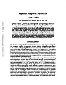
2. BAYESIAN ADAPTIVE EXPLORATION BAE iterates an Observation–Inference–Design cycle depicted in Figure 1. In the observation stage, new data are obtained based on an observing strategy produced by the previous cycle of exploration. The inference stage synthesizes the information provided by previous and new observations to assess hypotheses of interest. This synthesis produces interim results such as signal detections, parameter estimates, or object classifications. Finally, in the design stage the results of inference are used to predict future data for a variety of possible observing strategies; the strategy that offers the greatest predicted improvement in inferences (subject to any resource constraints) is passed on to the next Observation–Inference–Design cycle. Bayesian statistics is used for both the inference and design stages. The inference stage uses the tools of Bayesian inference. In particular, Bayes’s theorem, which combines prior information and data to produce posterior probabilities for hypotheses of interest, provides a formal description of learning perfectly suited for the tasks of the inference stage. The design stage uses Bayesian decision theory to find an optimal experimental or observational design by first specifying the purpose for a study, and then comparing how well candidate designs achieve that purpose by using the information in existing data to predict future data, and then determining how that data might improve inferences. Bayesian design can rigorously and straightforwardly account for uncertainties in assessing a design even in challenging settings (strongly nonlinear models, non-Gaussian noise). It interfaces naturally with Bayesian inference, so the tools of the inference and design stages work synergistically together.

162

PHYSTAT2003, SLAC, Stanford, California, September 8-11, 2003

Prior information & data Strategy

Observ’n

Combined information New data

Inference Predictions

Design

Strategy

Interim results Figure 1: Information flow through one cycle of the adaptive exploration process.

The main ideas of Bayesian inference will be familiar to many readers of this volume, but Bayesian experimental design is not a common tool in the physical sciences, so this brief report will focus on describing the key elements of the design stage (see Chaloner and Verdinelli [1995] for a review of Bayesian experimental design and references). As already noted, Bayesian design is an application of Bayesian decision theory. In decision theory an optimal decision is made in the face of uncertainty by enumerating the possible actions, a (e.g., whether to bet on heads or tails in a coin flip), and the possible outcomes, o, of which we are uncertain (e.g., which side of the coin will come up), and assigning a utility U (o, a) to action a if the outcome turns out to be o (e.g., the amount won or lost). If the available information, I, gives probability p(o|I) to outcome o, then thePexpected utility associated with action a is EU (a) = o p(o|I)U (o, a). Decision theory specifies that the optimal action is the one that maximizes the expected utility. In Bayesian design, the space of actions is the space of possible experiments or observations (e.g., the location in time or space for the next sample). The uncertain outcome is the data one would get performing a candidate experiment. An optimal design is found by specifying a utility and maximizing the expected utility. In some settings (e.g., financial or medical experiments), there may be a natural utility function associated with actual costs associated with outcomes. This is seldom true in physics experiments where the goal is simply to gain knowledge about a phenomenon. In 1956, Lindley described how one could use tools from information theory and Bayesian statistics to find optimal designs for achieving such a goal. He later incorporated these ideas into a more general theory of Bayesian experimental design, described in his influential 1972 review of Bayesian statistics (Lindley [1972]). This theory unifies and generalizes nonBayesian methods for optimal design that predated Lindley’s work (see Chaloner and Verdinelli [1995] for discussion of the relationships between Bayesian and non-Bayesian design). Lindley’s idea is to use information as utility, with information quantified via information theory. Thus the utility for experiment e (described in the background information, Ie ) producing data d is the nega-

tive entropy of the posterior distribution for the quantities (hypotheses) of interest, Hi : X p(Hi |d, Ie ) log [p(Hi |d, Ie )] . (1) I(d, e) = i

The optimal experiment maximizes the expected information, X X p(Hi |d, Ie ) log [p(Hi |d, Ie )] , p(d|Ie ) EI(e) = i

d

(2) where p(d|Ie ) is the predictive distribution for the data which can be calculated using X p(Hi |Ie )p(d|Hi , Ie ), (3) p(d|Ie ) = i

where p(Hi |Ie ) is the prior distribution for Hi given the current information, Ie (when some data is already available in Ie , this is the posterior distribution incorporating that data), and p(d|Hi , Ie ) is the sampling distribution for the future data. Finding optimal designs using EI(e) requires calculating a triply-nested set of sums or integrals for each candidate design, a computationally challenging task unless the integrals are analytic. Two recent developments finally allow application of this approach to settings of realistic complexity in the physical sciences, where the needed integrals are not analytic. First is the development of sampling-based methods for calculating probability integrals like those appearing here. Physicists are familiar with such methods for calculating integrals over sample space via Monte Carlo generation of simulated data (e.g., for the d sum in (2)). The new spin on this has been the creation of good Monte Carlo algorithms for hypothesis space integrals, where the distributions one must sample from are multidimensional and with complicated structure. These are the Markov chain Monte Carlo (MCMC) methods now widely used for Bayesian inference. Muller and his colleagues have pioneered application of MCMC methods to Bayesian design (Muller [1999]). The second development is the recognition that significant analytical simplification is possible in a restricted but common and very useful setting. It is often the case that the information in the sampling distribution, p(d|Hi , Ie ), is independent of Hi . That

163

PHYSTAT2003, SLAC, Stanford, California, September 8-11, 2003

is, roughly speaking, the width of the noise distribution does not depend on the properties of the underlying signal. This is the case when noise is additive and is dominated by detector or background sources. Sebastiani and Wynn [2000] showed that when this is true, the expected information simplifies, Z EI(e) = C − dd p(d|Ie ) log[p(d|Ie )], (4) where C is a constant (measuring the e-independent information in the prior and the sampling distribution). Thus the experiment that maximizes the expected information is the one for which the predictive distribution has minimum information, or maximum entropy. The strategy of sampling in this optimal way is called maximum entropy sampling. Colloquially, this strategy says you will learn the most by sampling where you know the least, an eminently sensible criterion. To flesh out these ideas, consider the problem of optimally scheduling observations of a star in order to characterize the orbit of a planet detected via radial velocity measurements of the Keplerian reflex motion of the star. The data are modeled by di = V (ti ; τ, e, K) + ei ,

(5)

where V (ti ; τ, e, K) gives the Keplerian velocity along the line of site as a function of time ti and of the orbital parameters τ (period), e (eccentricity), and K (velocity amplitude); for simplicity three purely geometric parameters are suppressed. This function is strongly nonlinear in all variables except K. Our goal is to learn about the parameters τ , e and K. Figure 2 shows results from a typical simulation iterating the BAE observation-inference-design cycle a few times. Figure 2a shows simulated data from a hypothetical “setup” observation stage. Observations were made at 10 equispaced times; the curve shows the true orbit with typical exoplanet parameters (τ = 800 d, e = 0.5, K = 50 ms−1 ), and the noise distribution is Gaussian with zero mean and σ = 8 m s−1 . Figure 2b shows some results from the inference stage using these data. Shown are 100 samples from the marginal posterior density for τ and e (one could smooth this distribution and present contours; this display illustrates the sampling approach behind the algorithm). There is significant uncertainty that would not be well approximated by a Gaussian (even correlated). Figure 2c illustrates the design stage. The thin curves display the uncertainty in the predictive distribution as a function of sample time; they show the V (t) curves associated with 15 of the parameter samples from the inference stage. The spread among these curves at a particular time displays the uncertainty in the predictive distribution at that time. A Monte Carlo calculation of the expected information vs. t (using all 100 samples) is plotted as

the thick curve (right axis, in bits, offset so the minimum is at 0 bits). The curve peaks at t = 1925 d, the time used for observing in the next cycle. Figure 2d shows interim results from the inference stage of the next cycle after making a single simulated observation at the optimal time. The period uncertainty has decreased by more than a factor of two, and the product of the posterior standard deviations of all three parameters (the “posterior volume”) has decreased by a factor ≈ 5.8; this was accomplished by incorporating the information from a single wellchosen datum. Figures 2e,f show similar results from the next two cycles. The posterior volume continues to decrease much more rapidly √ than one would expect from the random-sampling “ N rule” (by factors of ≈ 3.9 and 1.8). Figure 3 provides a further example motivated by the problem of detecting buried land mines using a mix of technologies—inexpensive but noisy ferromagnetic scans, and more costly but more sensitive acoustic scans using laser doppler vibrometry. Figure 3a shows a hidden 1-d Gaussian (dashed curve; peak at x0 = 5.2, amplitude A = 7, FWHM = 0.6) barely detected in an initial scan with 11 crude (σ = 1) observations spaced well over a full-width apart. Figure 3b shows samples from the marginal posterior density for A and x0 from the first inference stage, with very substantial uncertainty. BAE proceeds, designing for subsequent more sensitive observations (σ = 1/3). The design stage produces the predictive distribution (thin curves) and entropy curve (thick curve; right axis) in Figure 3c, suggesting observing near the best guess for the peak. A simulated observation produces the more concentrated but complicated Cycle 2 inference of Figure 3d. Two subsequent cycles identify optimal sample locations that flip-flop to either side of the peak, producing the Cycle 3 and Cycle 4 inferences of Figures 3e and 3f. The posterior volume decreases by factors of ≈ 8.2, 6.6, and 5.6 between cycles, far more dramatically than expected from random sampling (even adjusting for the fact that only two of the original samples lie in the signal region). The final posterior distribution is nearly uncorrelated and simple in shape. If for the last step one samples just a few tenths of a unit from the optimal point, the posterior volume is 40% larger and remains strongly correlated. These examples demonstrate the potential of BAE (and Bayesian design more generally) to greatly improve the return from planned experiments. But many issues must be addressed before the approach can be used efficiently and with confidence, including: adapting the algorithm to changing goals (e.g., from signal detection to signal characterization once the signal is detected); assessing robustness to model uncertainty (a possible “Achilles heel” in many settings); generalizing the utility to incorporate factors such as the cost of observations (financial or temporal); and finding good algorithms for higher dimensional models.

164

PHYSTAT2003, SLAC, Stanford, California, September 8-11, 2003

Figure 2: Results from various stages along four observation-inference-design cycles characterizing the orbit of an extrasolar planet with simulated radial velocity observations.

Figure 3: Results from various stages along four observation-inference-design cycles characterizing a hidden 1-d Gaussian object with simulated noisy observations.

Acknowledgments I thank David Chernoff and Paul Goggins for key input to this work. This work was supported by NASA through grant NAG5-12082 and the SIM EPIcS Key Project.

References T. J. Loredo, “Bayesian Adaptive Exploration,” in Maximum Entropy and Bayesian Methods, Jackson Hole, Wyoming, 2003, edited by G. Erickson and

Y. Zhai (Kluwer Academic Publishers, Dordrecht, 2004), in press. K. Chaloner and I. Verdinelli, Stat. Sci. 10, 273 (1995). D. V. Lindley, Bayesian statistics–a review (SIAM, Philadelphia, 1972). P. Muller, in Bayesian Statistics 6, edited by J. O. Berger, J. M. Bernardo, A. P. Dawid, and A. F. M. Smith (Oxford U. Press, 1999), pp. 459–474. P. Sebastiani and H. P. Wynn, J. Roy. Stat. Soc. B 62, 145 (2000).

165