17th European Signal Processing Conference (EUSIPCO 2009)
Glasgow, Scotland, August 24-28, 2009
SPARSE MODEL FITTING IN NESTED FAMILIES: BAYESIAN APPROACH VS PENALIZED LIKELIHOOD Laure Amate and Maria João Rendas Laboratoire I3S, UNSA/CNRS 2000 route des lucioles BP 121, 06903, Sophia Antipolis, France phone: + (33) 4 92 94 27 71, fax: + (33) 4 92 94 28 98, email: amate,
[email protected] web: www.i3s.unice.fr
ABSTRACT We study the problem of model fitting in the framework of nested probabilistic families. Our criteria are: (i) sparsity of the identified representation, (ii) its ability to fit the (finite length) data set available. As we show in this paper, current methodologies, often taking the form of penalized versions of the data likelihood, cannot simultaneously satisfy these requirements, as the examples presented clearly demonstrate. On the contrary, maximization of the Bayesian model posterior, even without assumption of a complexity penalizing prior, is able to select models with appropriate complexity, enabling sound determination of its parameters in a second step. 1. INTRODUCTION
over Θ, and optimize the expected value of some functional of the estimation error under the posterior distribution over Θ. Set (3) no longer has the structure of a vector space, even when each Θk is a vector space. Definition of distributions which are the basic entities manipulated by Bayesian techniques (e.g. prior or posterior distributions) must be done with care. When parametric probabilistic families over each Θk are known, as we assume her, an intuitive way is to use a mixture-like approach, writing densities over Θ as p(θ ) =
M
=
∪
Mk
;
K = {kmin · · · kmax }
(1)
k∈K
Mk
= {p(·|θ ), θ ∈ Θk } ⊂ Mk+1 .
∪
Θk .
(3)
k∈K
To make the problem stated above tractable, we need to specify what “correctly” means, i.e., to define the criterion that the selected model pˆ = p(·|θˆkˆ ) must optimize. Two common choices for parameter estimation are Maximum Likelihood (ML) and Bayesian. It is well known that ML is inconsistent for models with this structure, systematically preferring the most complex models. Bayesian approaches regularize the identification problem through the definition of a prior
© EURASIP, 2009
θ ∈Θ ,
(4)
1≥
∫ Θk
pk (θ )d θ ≡ Pr(Mk ) .
A proper density νk (θ ) over Θk is obtained by normalization: pk (θ ) ≡ p(θ |Mk ) , θ ∈ Θk , Θk pk (θ )d θ
νk (θ ) , ∫
where we stressed the meaning of νk as resulting from conditioning on θ ∈ Θk . Note that these “local” densities (as their un-normalized versions) are defined w.r.t distinct reference measures, the invariant measures, over each Θk and are thus not directly comparable. 1.2 Background
(2)
The integer k indexing each family of models Mk is directly related to their complexity: if k0 > k, the complexity of models in Mk0 is higher than the complexity of those in Mk . The overall parameter space Θ of M is simply Θ=
pk (θ ),
where each pk (θ ) is the Radon-Nikodym derivative of an unnormalized measure with respect to (w.r.t) the invariant measure over Θk : if θ ∈ / Θk then pk (θ ) = 0, and
1.1 Problem formulation In many situations of interest the ultimate goal is to identify one simple model that “correctly” describes the structure of the observed data Z. One can then discard the original data using the identified model as a proxy for it. This is different from denoising-like problems, where we are not interested in learning the data structure, but rather to “clean it”. Generally speaking, the complexity of a model is a measure of the information needed to specify it. A convenient way of adjusting the model complexity to the data complexity is to consider a set M of candidate models that is the union of nested families of parametric models Mk :
∑
k∈K
To correct the overfitting behavior of ML, many authors proposed the addition of corrective terms that favor selection of models using less parameters:
θˆPL = arg max p(Z|θ ) + P(k) , k,θ
(5)
where P(k) is a decreasing function of k. These techniques are generally known by the name of “penalized likelihood” methods, and have received three distinct justifications. (i) They are sometimes dictated by the desire to impose some regularity characteristics on the solution, requiring in this case prior knowledge on its characteristics which is not necessarily available. (ii) They have also been justified as particular cases of MAP (Maximum a Posteriori) estimation for special selections of the prior p(θ ), e.g. in [2, 4]. We will see below that there is a fundamental flaw in this approach. (iii) More generically, they are derived from
2628
asymptotic arguments which relate them to the models’ Bayesian marginal posterior [9] Pr(Mk |Z) – this is the case for AIC (Akaike Information Criterion), BIC (Bayesian Information Criterion) and MDL (Minimum Description Length) – [13, 12], and thus cannot offer any guarantee for finite data sets. As we see, generic justifications of penalized likelihood link it to Bayesian estimates: either to the model posterior p(θ |Z) or to the marginal model posteriors Pr(Mk |Z). Let us concentrate first on Bayesian estimates for θ . The two most popular Bayesian criteria are the MMSE (Minimum Mean Square Error) and the MAP (Maximum A Posteriori). For the union-type models like (1)-(2)-(3), the MMSE criterion is meaningless, the associated cost function (θ − θˆ (Z))2 being undefined when θ ∈ Θk and θˆ (Z) ∈ Θk0 with k 6= k0 . On the contrary, the 0/1 cost function of the MAP criterion is well defined, and should enable determination of a unique model amongst the set of candidate models. When Θ has the simple structure of a vector space, this criterion leads to θˆ (Z) = arg maxθ p(θ |Z). Surprisingly, several authors have proposed estimators based on a direct transposition of this equation to the model structure considered herein [1, 4]. We designate them by “naive MAP” estimators:
θˆnMAP = arg max p(θ |Z) = arg max max pk (θ |Z) (6) θ ∈Θ
k∈K θ ∈Θk
= arg max pk (θˆk |Z) , k∈K
θˆk
= arg max pk (θ |Z) θ ∈Θk
As we pointed out before, the un-normalized densities pk (θ |Z) defined over each Θk are not defined with respect to the same measures. This criterion, that abusively compares them directly, may lead to estimates with pathological behavior as the examples given below demonstrate. We address now the second justification of penalized likelihood, that relates it to Bayesian Model Selection (BMS) which does not attempt at directly selecting the model set and the parameter value, and instead starts by selecting the model Mk using the posterior probabilities Pr(Mk |Z), k ∈ K [14]: ∫
kˆ = arg max k
Θk
p(θ |Z) d θ .
(7)
Determination of these posteriors requires specification of a priori distribution π defined over Θ, that if π is of the form (4) implies ∀k ∈ K , p(Z|Mk )π (Mk ) , ∑ p(Z|M j )π (M j )
Pr(Mk |Z) =
(8)
j∈K
∫
Pr(Z|Mk ) =
p(Z|Mk , θk ) π (θk |Mk )d θk .
whether this marginal approach can guarantee the aptitude of the elements of Mkˆ , alone, to fit the data well. We will see below that in all the examples considered the models selected by BMS have fitting properties close to those obtained by penalized likelihood criteria. More surprisingly, numerical studies not reported here show that their fitting performance in “signal-in-noise” problems is similar to direct MMSE “signal” estimation, which belongs to a set much richer than M . 1.3 Numerical issues For most problems of practical interest Bayesian approaches must resort to numerical (Monte Carlo) methods [3, 7]. A tool that has now become a standard to draw from posteriors p(θ |Z) with the structure (1)-(2) is RJMCMC (Reversible Jump Markov Chain Monte Carlo) [8]. It builds a Markov Chain over Θ that asymptotically converges to p(θ |Z), enabling numerical determination of expected values with respect to it. Models with the structure (1)-(2)-(3) often occur in the search for a parsimonious parametric model f (t; θ ) for a signal s(t) of which we observe noisy samples: Z(ti ) = s(ti ) + ε (ti ) ' f (ti ; θ ),
We refer to [9] for some analysis about how one can specify the prior. Once the model is determined, the parameter θ ∈ Θkˆ can be estimated using one of the standard statistical estimation criteria (ML, MMSE, MAP,...). This (sound) estimation approach selects k by comparing the total posterior probability mass accumulated over Mk . One may question
(10)
where the distribution of the noise ε (t) is known. For this problem BARS (Bayesian Adaptive Regression Splines) [6] uses RJMCMC to find an estimate of s(t) as E[ f (t; θ )| Z], giving up identification of a single parametric model for s(t). In [2, 1], Reversible Jump Simulated Annealing (RJSA, a Simulated Annealing (SA) algorithm with a proposal distribution controlled by a RJMCMC kernel) is used to find the maximum of the “posterior density” in (6). We can also mention the trans-dimensional simulated annealing (TDSA) of [4], that maximizes a penalized likelihood interpreted by the authors as a “posterior over Θ”. 1.4 Outline In our (large) introduction, we concluded that only BMS can serve as a sound method for model identification using nested model families. In section 2 we describe a numerical implementation of BMS for problem (10), that first computes the marginal MAP criterion and then identifies a model within the family of models chosen previously using a standard MAP criterion. Section 3 illustrates the possible pathological behavior of the “naive MAP” estimator (6) – directly relating it to the varying dimension of the parameter sets Θk – in a simple case-study where analytical determination of the posterior is possible. The last section compares use of the BIC penalty to the actual computation of the BMS criterion within the context of free-knots splines curve modeling, revealing its biased behavior for small data sets.
(9)
Θk
i = 1···N .
2. TWO-STEP MAP ESTIMATION We present now a numerical implementation of the “Twostep MAP estimator”,
2629
(i) kˆ = arg max Pr(Mk |Z) ,
(11)
(ii) θˆ = arg max p(θ |Z, Mkˆ ) .
(12)
k∈K
θ ∈Θkˆ
that uses BMS to select Mk and MAP to identify a θ ∈ Θkˆ . In this manner optimization is done in each step using commensurable score functions: the (discrete) posterior distribution over the families of models Mk in (i), and a regular posterior density over Θkˆ , with respect to a selected base measure, in (ii). Note that [10] proposes a similar idea for ML estimation, selecting first the Mk using the BMS criterion and computing the ML estimates of the θ ∈ Θk in a second step. We consider a prior π of the form (4),
πθ (θ ) =
kmax
∑
π (θ |Mk ) Pr(Mk ),
2.1 Identification of Mk (family selection) For most problems the posterior probabilities Pr(Mk |Z) have no closed-form and their maximum must be determined nuˆ merically. We obtain estimates Pr(M k |Z) by sampling from p(θ |Z), θ ∈ Θ using RJMCMC [8] and computing the total mass of each Mk as the corresponding marginals. RJMCMC uses a proposal distribution q(θ 0 |θ ), θ 0 ∈ Θk0 , θ ∈ Θk , where θ (resp. θ 0 ) is the current (resp. candidate) state of the chain, that is a mixture of basic transition distributions (birth, death or change) moving across neighboring families of models Mk and Mk+1 . To ensure chain reversibility (and thus convergence in distribution to the target distribution p(θ |Z)) the acceptance function of the chain is [8] αRJ (θ , θ 0 ) = min {1, rRJ }, with p(θ 0 |Z) q(θ 0 |θ ) J(θ 0 , θ ) , p(θ |Z) q(θ |θ 0 )
(13)
where J(θ 0 , θ ) is the Jacobian of the mapping from θ to θ 0 . Finally, the family Mkˆ is chosen using the RJMCMC sam( ) (i) M ∝ p(θ |Z) in the following manner ples θk(i) i=1
Mk ˆ Pr(M , (14) k |Z) = M } (i) : k = k (# A is the cardinality
ˆ kˆ = arg max Pr(M k |Z), k
{( where Mk = #
(i)
θk(i)
)M i=1
0.6 0
1 0.25
1.2 0.61
1.6 0.945
2 0.985
4 1
Table 1: Pr(θ˜ ∈ M1 |M2 ), σ 2 = (0.6, 1, 1.2, 1.6, 2, 4). 3. NAIVE MAP: PATHOLOGICAL BEHAVIOR In this section we expose using a simple example the possible biased behaviour of the “naive MAP” criterion. 3.1 Case-study
θ ∈Θ .
k=kmin
rRJ =
σ2 ˜ Pr(θ ∈ M1 |M2 )
of set A). 2.2 Estimation of θ (parameter estimation) Once the family Mkˆ has been determined, parameter estimation is done for θ ∈ Θkˆ . Again, there is, in general, no analytical solution, and we must resort to a numerical method to find the model with the maximal posterior density pkˆ (θ |Z). A common choice for approximating the solution of this optimization problem is Simulated Annealing (SA), with an acceptance probability αSA : ( )1 0 T i p(θkˆ |Z, Mkˆ ) αSA (θkˆ0 , θkˆ , Ti ) = min 1; , (15) p(θkˆ |Z, Mkˆ ) where θkˆ (resp. θkˆ0 ) is the current (resp. candidate) state, and Ti is the chain temperature that must decrease according to a convenient cooling scheme. We refer the interested reader to [11] for details on SA.
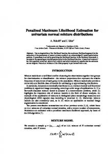
Let Z = [z1 , . . . , zn ] ∈ Rn be the observation vector, and consider a model with just two families: M = M1 ∪M2 , where1 { ( ) } Mk = N fk (·|θ ), σ 2 In , θ ∈ Θk , k = 1, 2 . Above, fk (·|θ ) is a k-piecewise linear signal, see Figure 1(a), such that the parameters of the models are θ1 = [P0 , σ 2 ] and θ2 = [P1 , P2 , σ 2 ], where {Pi = (Pxi , Pzi ) ∈ R2 }2i=0 are the break point coordinates. We use an uninformative factored prior distribution over both parameter spaces: Pxi ∝ U ([0 N]), Pzi ∝ N (0, Σ2 ), i = 0, 1, 2, and σ 2 ∝ U (R+ )2 . To minimize the impact of the prior we set Σ2 À 1. Models are equiprobable: π (M1 ) = π (M2 ). 3.2 Naive MAP estimator Apparently, the prior chosen does not express preference for M1 , and one would expect that the biased ML behaviour (always choose M2 ) would not be corrected. We will see that this is not the case, and that a bias of opposite sense is induced, (6) exhibiting a strong preference for the simpler model M1 . ( Table 1 displays ) estimates of the error probability Pr θˆ ∈ Θ1 |θ ∈ M2 for several values of the noise variance σ 2 , obtained over 200 Monte Carlo runs. Parameters were set at: P1 = (250, 10), P2 = (800, 6), Σ = 1016 and X = {10m}100 m=0 , see figure 1(b). We see that even for small values of the noise variance the error probability is very high: the “naive MAP” estimator is biased toward the simplest model M1 , even if the data clearly shows the existence of 3 different slopes. We will now show that this preference for simple models 8
12
7 10
6 8
5 6
4 4
3 2
2
0
1
0
0
100
200
300
400
500
(a)
600
700
800
900
1000
−2
0
100
200
300
400
500
600
700
800
900
1000
(b)
Figure 1: (a) f (·|θ1 ) (− blue), f (·|θ2 ) (−− red) ; (b) Z ∝ p(·) ∈ M2 , σ 2 = 1.2. 1 N ( µ , Σ) denotes the normal density with mean µ and covariance matrix Σ. 2 X ∝ p indicates that random variable X is drawn according to p and U (A) denotes the uniform distribution over set A.
2630
that seems to be hidden in the prior chosen is actually an artifact caused by the comparison of densities defined with respect to distinct measures. Let ρi2 = ||Z − fi (X; θi )||2 be the residuals for model Mi , i = (1, 2). Criterion (6) leads M1
to a model selection rule r ≶ 1 where r is the ratio M2
This scheme is adapted to find the MAP estimates of the parameters θ ∈ Θk for fixed k. In this case, the target distribution of SA algorithm is the posterior p(θ |Z, Mk ). We use the factored prior already proposed for this problem in [6], except for the prior over k which we consider uniform, establishing thus no prior preference for simpler models:
π (M2 ) p2 (θ2 |Z) π (M1 ) p1 (θ1 |Z) √ ( ) ) ( (P1 )2 + (Pz2 )2 − (Pz0 )2 2 1 ρ1 n = exp − z . π ΣN ρ2 2Σ2 ( ) (P1 )2 +(Pz2 )2 −(Pz0 )2 If Σ2 À 1, such that exp − z ' 1, then 2Σ2 r
=
π (θk ) = π (βk |Mk , ξk , σ 2 ) π (ξk |Mk ) π (Mk ) π (σ 2 ).
( √ ) ) ρ1 M1 1 π log ≶ log ΣN = γ. ρ2 M2 n 2 (
Note that ΣN is the ratio of the normalizing constants of the prior densities over Θ1 and Θ2 , that increases with the number of breakpoints of M2 . As the previous equation shows, the decision region for M1 increases monotonically with ΣN, explaining why the apparently uninformative prior leads to a strong bias in favor of M1 . This biased behaviour is entirely due to the fact that we are comparing the “densities” pk (·|Z) defined with respect to measures µk (the Lebesgue measure in both cases) over spaces of distinct dimensions (d1 = 3, d2 = 5). Depending on the priors chosen, this may bias the decision, in an unclear manner, in favor of simpler or more complex models. We stress that these remarks do not concern penalized likelihood methodologies globally, but only their interpretation as Bayesian MAP estimators. 4. BIC AND BAYESIAN MODEL SELECTION In this section, we compare BIC to the two-step BMS/MAP semi-parametric identification described in section 2 for curve modeling with free-knot (cubic) splines. We begin with a brief description of the model and of numerical issues related to its optimization, presenting our comparative study in a second step. 4.1 Free-knots spline model We assume that the observations follow a normal model p(Z|θ , Mk ) = N
(
)
f (t; θ ), σ 2 I ,
a factor of 0.2. The maximum number of iterations is fixed to 10000. We thus obtain the ML estimate of the parameter vector (with k fixed). Adding the BIC penalty term to the likelihood and maximizing the sum with respect to k allows determination of the BIC-penalized estimate of k.
k π (Mk ) = U (k ∈ [kmin(, kmax ]); π (ξk |M ) k ) ∼ U ([0 1] ); 2 2 T −1 π (βk |Mk , ξk , σ ) = N 0, σ N(B B) where B = Bk,ˆ ξ is the spline design matrix with entries bi (t, ξk ); π (σ 2 ) = 1/σ 2 . As described in section 2, we first identify Mkˆ , using RJMCMC to estimate Pr(Mk |Z). The proposal distribution q(θ 0 |θ ) is classically taken as a mixture of basic transition laws that allow “jumps” between families of models: birth (b), death (d) and change (c) of a knot point in the knot vector ξk . With these priors, holding ξk fixed, we can analytically find the MAP estimates of the linear coefficients βk and of the noise variance σ 2 . We obtain one sample of the parameter vector at each iteration of the RJMCMC procedure, allowing thus the numerical determination of kˆ for the criterion (14). ˆ the second step identifies the parameFixing k = k, ters of Mkˆ by maximizing the “local posterior density” νk (θ ) = p(θ |Z, Mkˆ ), θ ∈ Θkˆ . Maximization with respect to (βkˆ , σ 2 ) can again be found analytically, see [6], enabling the definition of the “reduced posterior” P(ξkˆ |Z, Mkˆ ) = p(ξkˆ |Z1N , Mkˆ )p(βˆkˆ , σˆ 2 |Z, Mkˆ , ξkˆ ). A SA algorithm is run with P(ξkˆ |Z, Mkˆ ) as the score function, producing a sequence of values of ξkˆ that converge in distribution to its maximum, completely identifying a single model amongst M . We performed M = 10000 iterations of the RJMCMC algorithm followed by L = 2000 SA iterations. Temperature Ti is initialized at T0 = 0.02, and is halved every 500 iterations.
4.3 Numerical results
k
f (t; θ ) = ∑ β i bi (t, ξk ) . i=1
(16) where k is the number of knots, bi (t, ξk ) is the ith B-Spline function, ξk ∈ [0 1]k is the (ordered) knots vector, and βk ∈ R2k is the vector of control points. We refer to [5] for details about splines. The parameter vector of Mk is θk = (ξk , βk , σ 2 ). 4.2 Implementation Maximization of the likelihood allows analytic determination of the estimates of βk and σ 2 for a fixed model order k. Using the reduced likelihood at this estimated values as the target distribution of the SA algorithm, we can find the ML estimate of the knot vector ξk . Temperature Ti is initialized at T0 = 50 and decreases every 500 iterations by
We first compare the two methods BIC and BMS/MAP on simulated data, with the goal of exposing the asymptotic nature of the BIC criterion, which only for very large data sets is an approximation of BMS, inheriting the problems of “naive Bayes” under its interpretation as a posterior computed for a particular “prior.” We simulated data from a spline model with k = 13 knots and σ 2 = 0.04 (see Fig. 2), and considered two observation sets: D1 with N = 51 data points and D2 with N = 401 data points, see Figure 2. Figure 3 summarizes the comparison of the two methods. For the shorter data set D1 BIC systematically chooses a ’wrong’ model order k = 12 (Fig. 3(left)), underestimating the data complexity, while BMS/MAP correctly identifies the true value k = 13 (Fig. 3(right)). For the larger data set D2 both criteria choose the same (and correct) model order, confirming that only asymptotically BIC yields an unbiased estimate of the model complexity, while the two-step
2631
2.5
BIC BMS/MAP
2
D1 0.0597 0.0620
D2 0.0848 0.0845
1.5
Table 2: Average (over 50 runs) of the mean square error between data and models.
1
0.5
0
user from the need to choose a specific penalty on the model dimension. The discussion in this paper shows that only a BMS twostep approach provides a safe methodology for identification with the type of models considered. The price payed for this better (unbiased) performance is an increase in the computational complexity of the estimation task. For the particular type of models used in the examples presented here (free knot splines), we think that a number of useful heuristics can be defined by exploiting the locality of the basis functions. We will address this issue in future publications.
−0.5
−1
−1.5
−2 −2.5
−2
−1.5
−1
−0.5
0
0.5
1
1.5
2
2.5
Figure 2: Spline model (-) and data sets D1 (*) and D2 (·). 10 0
9 −50
8
7
−100
REFERENCES
6 −150
5 −200
4
3
−250
2 −300
1
−350
8
10
12
14
16
18
20
22
24
26
8
9
10
11
12
13
14
15
Figure 3: (left) BIC criterion for D1 (−−) and D2 (−) depending on the model order in abscissa. (right) Log-posterior probability of models for D1 (black) and D2 (gray) with model order in abscissa. numerical estimator BMS/MAP has an unbiased behavior for all values of N. Table 2 shows the mean square error of the models identified by the two criteria, averaged over the 50 MC runs. We note here that while producing overall similar error figures, for the larger data set D2 the two models have indeed virtually identical residual error, while for D1 BIC yields a slightly smaller error, revealing its close relation to ML. 5. CONCLUSION This paper draws a comparative analysis of several approaches proposed in the literature for semi-parametric estimation in the context of model fitting using nested families of models. We concentrate in statistically based methodologies related to the use of penalized versions of the likelihood score and their frequent interpretations either as maximizing the model parameter “posterior distribution” or as asymptotic approximations of the marginal posterior probabilities of each model family. We stress a basic flaw of direct transposition of the MAP criterion to this complex setting as it has sometimes been done in the literature – and thus of the former interpretation of penalized likelihood – showing in a simple problem that it can lead to arbitrarily biased estimates. We then discuss the potential problems associated with asymptotic penalties, showing that the same negatively biased behavior can occur when the data set is of finite length, while computation of the true model posterior leads to unbiased estimates of the model complexity. Underestimating the model complexity for smaller data sets, BIC may fail to capture important structure of the data. As our example shows, even under a uniform prior over the models, use of the correct Bayesian criterion is not subject to the overfitting behavior typical of likelihood scores, relieving the
[1] C. Andrieu, N. de Freitas, and A. Doucet. Reversible jump mcmc simulated annealing for neural networks. In UAI ’00: Proc. of the 16th Conference on Uncertainty in Artificial Intelligence, pages 11–18, San Francisco, CA, USA, 2000. [2] C. Andrieu, N. D. Freitas, and A. Doucet. Robust full bayesian learning for radial basis networks. Neural Comput., 13(10):2359–2407, 2001. [3] C. M. Bishop. Pattern Recognition and Machine Learning (Information Science and Statistics). Springer, August 2006. [4] S. P. Brooks, N. Friel, and R. King. Classical model selection via simulated annealing. Journal Of The Royal Statistical Society Series B, 65(2):503–520, 2003. [5] C. DeBoor. A Practical Guide to Splines. Springer, 1978. [6] I. DiMatteo, C. Genovese, and R. Kass. Bayesian curve-fitting with free-knot splines. Biometrika, 88:1055–1071, 2001. [7] W. R. Gilks, S. Richardson, and S. D. J. Markov Chain Monte Carlo in Practice. Chapman & Hall/CRC, 1995. [8] P. J. Green. Reversible jump markov chain monte carlo computation and bayesian model determination. Biometrika, 82:711–732, 1995. [9] R. E. Kass and A. E. Raftery. Bayes factors. Journal of the American Statistical Association, 90:773–795, 1995. [10] M. Kliger and J. M. Francos. Map model order selection rule for 2-d sinusoids in white noise. IEEE Transactions on Signal Processing, 53(7):2563–2575, 2005. [11] R. H. J. M. Otten and L. P. P. P. van Ginneken. The Annealing algorithm. Kluwer Academic, 1989. [12] J. Rissanen. Modeling by shortest data description. Automatica, 14:465–471, 1978. [13] G. Schwarz. Estimating the dimension of a model. The Annals of Statistics, 6(2):461–464, 1978. [14] L. Wasserman. Bayesian model selection and model averaging. J Math Psychol, 44(1):92–107, March 2000.
2632