Multiplicative algorithms for maximum penalized likelihood inversion

Multiplicative algorithms for maximum penalized likelihood inversion with nonnegative constraints and generalized error distributions Jun Ma Department of Statistics, Macquarie University Sydney, Australia E-mail: [email protected]

Abstract.

In many linear inverse problems the unknown function f (or its discrete approximation

θ p×1 ), which needs to be reconstructed, is subject to the nonnegative constraint(s); we call these problems the nonnegative linear inverse problems (NNLIPs). This paper considers NNLIPs. However, the error distribution is not confined to the traditional Gaussian or Poisson distributions. We adopt the exponential family of distributions where Gaussian and Poisson are special cases. We search for the nonnegative maximum penalized likelihood (NNMPL) estimate of θ. The size of θ often prohibits direct implementation of the traditional methods for constrained optimization. How to develop easy-to-implement algorithms for the NNMPL estimates is an interesting and challenging question. Given that the measurements and point-spread-function (PSF) values are all nonnegative, we propose a simple multiplicative iterative algorithm. We show that if there is no penalty, then this algorithm is almost sure to converge; otherwise a relaxation or line search is necessitated to assure its convergence. Key Words: Nonnegative linear inverse problems; Multiplicative iterative algorithms; Maximum penalized likelihood.

Submitted to: Inverse Problems

Multiplicative algorithms for MPL inversion

2

1. Introduction NNLIPs exist in many different areas.

A few examples are: medical image reconstruction from

projections, such as single photon emission computed tomography (SPECT) and positron emission tomography (PET) (e.g.

[34] and [15]); seismic data deconvolution (e.g.

[21]); image or signal

restorations with nonnegative constraints (e.g. [37], [17] and [16]); inference of HIV infection rate from AIDS incidence data (e.g. [3]). Often, the unknown function f (or its discrete approximation θ p×1 ), which needs to be reconstructed, is subject to the nonnegative constraint f ≥ 0 (or θ ≥ 0 which means all elements of θ are nonnegative). [7] establishes that convex-set constraints help improve reconstruction quality and [22] contains mass spectrometry examples demonstrating that significant quality improvement over unconstrained reconstructions can be realized. To simplify discussions let us only consider, to begin with, the discrete approximation θ. Since the size of θ is commonly very large, the traditional textbook methods for constrained optimization, such as those given in [19, Chapters 10 - 12], become less feasible. In practice, the following methods are frequently used for enforcing the nonnegative constraints on maximum likelihood (ML) or maximum penalized likelihood (MPL) estimates of θ. The first approach assumes θ = u(γ) (e.g. θ = exp(γ)), where vector γ is unconstrained and u a predefined (one-to-one or many-to-one) function, such that each θj is nonnegatively constrained, due to function u, on all finite values of γ. Then unconstrained algorithms are developed for maximizing likelihood or penalized likelihood with respect to γ; see [37] and the references therein. The second approach imposes the nonnegative constraints on estimates of a given algorithm by projecting the updates of each iteration onto the positive orthant, i.e. replace the negative estimates with a small threshold value (or zero). We call this the “reset to zero” method. As has been commented in [16], this procedure cannot be used if the definition domain of the objective function is not the full space. Our Example 1 of Section 5 also confirms this. Recently, Ahn and Fesller ([1]) suggest algorithms for reconstructions in emission tomography using relaxed ordered subsets. In these methods they use “reset to zero” in each subiteration to facilitate the positive constraints and the resulting algorithms have global convergent property. The third approach embeds the nonnegative constraints (and simultaneously, other restrictions such as smoothness) directly into the penalty function, such as a cross-entropy penalty [22] or an independent Gamma penalty [35, 14] or others [23], and then use an unconstrained algorithm to estimate θ. The fourth approach is the iterative coordinate ascent (ICA) method which was first proposed for MPL reconstruction in emission and transmission tomography; see, e.g. [4]. Briefly, in each iteration, the method updates each element of θ by first expressing the objective function as a function of that unknown element and then applies Newton’s (or other) method to find a constrained optimal solution (which is trivial) to this univariate function. There also exists, in the literature, other constrained algorithms for maximizing objective functions rather than the likelihood or the penalized likelihood. Some examples are [26], [6], [36] and [11].

Multiplicative algorithms for MPL inversion

3

However our focus in this paper is on constrained (nonnegative) MPL reconstructions. We are motivated to develop easy-to-implement inversion algorithms, particularly algorithms with multiplicative format, for NNMPL estimates. Eggermont [8] discusses the particular importance of multiplicative algorithms among general iterative algorithms for positively constrained ML estimates. Before introducing our method, we first provide a brief summary of multiplicative algorithms in imaging and signal processing fields. Vardi and Lee [33] suggest a positive inversion method which relates closely to the Expectation-Maximization (EM) algorithm and can be interpreted as providing the ML estimate when model noise adopts a Poisson distribution. Archer and Titterington [2] propose the use of an image space reconstruction algorithm (ISRA) for positive linear inverse problems, which can be explained as searching for the ML solution when model noise follows a Gaussian distribution. However both methods, when applied to maximizing a penalized likelihood function, cannot guarantee positive MPL estimates. Lant´eri et al [16] develop a general multiplicative algorithm for NNLIPs, and, in fact, the method we propose in Section 3 can be viewed as a particular case of their method. The deblurring algorithm of Synder et al [30] uses Csisz´ar’s I-divergence measure as the objective function in the minimization procedure. This measure is closely related to the Kullback divergence (or crossentropy) and to the negative Poisson log-likelihood function; the resulting algorithm is identical to that of Vardi and Lee [33]. A common characteristic of the above methods is that they mainly consider Gaussian or Poisson noise processes. Our method in Section 3 covers more general error distributions. The rest of this article is organized as follows. An introduction to a nonnegative linear inverse problem (NNLIP) with generalized error distribution is given in Section 2. Section 3 develops our multiplicative iterative inversion algorithms with convergence properties studied in Section 4. Two examples are given in Section 5 and discussions and conclusion remarks are in Section 6. In the following discussions, for any function g(·), expressions g 0 and g 00 denote the first and second derivatives of g with respect to the argument in the bracket. 2. NNLIPs with generalized error distributions Suppose there is a mathematical model associating an input-output system. A direct problem consists of predicting the output from the input, while an inverse problem is to determine the input from the observed output. By a NNLIP we mean both input and output are nonnegative valued; see [33]. Usually, because observations are noise contaminated, statistical inversion methods are preferred, as they use appropriate probability models to describe the noise. In this paper we assume that the noise follows a distribution in the exponential family, which contains Gaussian and Poisson distributions as special cases; this specifies a NNLIP with generalized error distributions. More specifically, we consider the following linear inverse problems. Suppose independent and nonnegative observations y1 , . . . , yn are obtained and they are linked to an unobserved, real valued,

Multiplicative algorithms for MPL inversion

4

nonnegative function f ∈ H by E(yi | f ) = Li f,

(1)

where Li : H → R1 , i = 1, ..., n, are linear functionals and H is a Hilbert space endowed with a well defined inner product. In this paper we adopt a discrete approximation to f , i.e. we estimate a p × 1 vector θ = (θ1 , . . . , θp )T , where the superscript T denotes matrix transpose, rather than f . Note that, in order for θ to be close to f , p must be large; see [12] for discussions on discretization methods and other conditions for making θ close to f . Functional Li is similarly discretized into a row vector Pn Ai = (ai1 , . . . , aip ) with aij ≥ 0 and i=1 aij > 0. Note the case of some aij < 0, such as the problem described in [28], is not of interest in this paper. Thus, after discretization, (1) becomes: E(yi | θ) = Ai θ.

(2)

Relationship (2) represents the systematic component of our inverse problem model, while the random component, which depicts the randomness (or noise) of observations, is determined by the probability density function p(yi | µi ). We assume p(yi | µi ) belongs to the exponential family of distributions, its log density function is given by log p(yi | µi ) =

1 {yi b(µi ) − c(µi )} + d(yi , φ), φ

(3)

where µi = E(yi | θ) and φ > 0 is the (usually unknown) scale parameter. Here we have reparameterized the density function using µi . It can be shown (e.g. [20, Chapter 2]) that the mean and the variance of yi are, respectively, µi = c0 (µi )/b0 (µi ) and var(yi | θ) = φ vi , where vi is called the variance factor given by vi = 1/b0 (µi ). Since µi and vi are both functions of θ, we may sometimes write them as µi (θ) and vi (θ) to emphasize this relationship. The following assumptions about p(yi | µi ) are made throughout the paper. Assumption 1 We assume that (i) The first two derivatives of b(µi ) and c(µi ) exist for µi in its domain. (ii) yi b(µi ) − c(µi ) is concave (as a function of µi ) for µi in its domain, i = 1, . . . , n. (iii) Whenever µi approaches the boundary of its domain, the value of yi b(µi ) − c(µi ) will converge, either to a constant or to −∞. (iv) The variance factors vi are nonzero, i.e. vi > 0 for i = 1, . . . , n. In practice, such as tomographic imaging, often for some i we have µi = 0.

In this case, as

vi = µi /c0 (µi ), it is possible that vi = 0 (unless c0 (µi ) is a linear function of µi , as in the Gaussian distribution case). Clearly µi = 0 only when aij θj = 0 for all j. Hence after setting θj = 0 for aij 6= 0, we can exclude index i from our computation, as the corresponding yi ’s do not contain useful information on nonzero θj . This treatment assures Assumption 1 (iv). An equivalent treatment (for the multiplicative iterative algorithm given in Section 3) is simply to replace any vi = 0 by vi = δ > 0, where δ is a small positive value, such as δ = 10−12 . The reason for this second approach is given in Section 3.

Multiplicative algorithms for MPL inversion Log density (3) contains many familiar distributions as special cases.

5 For example, when

b(µ) = log(µ), c(µ) = µ and φ = 1 it gives the Poisson distribution with mean µ; if b(µ) = µ, c(µ) = µ2 /2 and φ = σ 2 then it is the Gaussian distribution with mean µ and variance σ 2 . For fixed p the model determined by (2) and (3) is simply the generalized linear model (GLM) of Nelder and Wedderburn [24] with identity link. But the standard estimation procedure of GLM is hardly useful here for three reasons. Firstly, p is usually large making conventional algorithms such as Newton-Raphson or Fisher scoring impractical. Secondly, many inverse problems are ill-conditioned, hence a regularization technique is necessary to stabilize the solution ( see [32]). Thirdly, parameters θ are nonnegatively constrained. We adopt a penalty function to regularize the estimate, i.e. θ is estimated by maximizing a penalized log-likelihood function, while the nonnegative constraints and large p are addressed by our multiplicative algorithm. Let Ω = {θ = (θ1 , . . . , θp )T ; θj ≥ 0, j = 1, . . . , p} ⊂ Rp be the feasible set for all possible θ. The interior of Ω is given by θ > 0 (i.e. all θj > 0 for j = 1, . . . , p) and is denoted by int(Ω). The log-likelihood function l(θ), apart from the terms independent of θ, is n 1 X {yi b(µi ) − c(µi )}, l(θ) = φ 1 and the penalized log-likelihood is lh (θ) = l(θ) − hJ(θ).

(4)

Function l(θ) measures the consistency between data y and its expectation µ and function J(θ) imposes some properties about θ, such as smoothness. J(θ) can be interpreted as the log of the prior distribution density of θ and, in this context, the MPL estimation is equivalent to the maximum a posteriori (MAP) method. There are many possibilities for J(θ), such as a quadratic function from the Gaussian prior or a function from the Gibbs prior. We call h ≥ 0 the smoothing parameter and J(θ) the penalty function. We use subscript h in the notation of the penalized log-likelihood function (i.e. lh (θ)) to emphasize its dependence on h. When h = 0, lh (θ) reduces to l(θ) and the corresponding estimate is ML. In this paper we are interested in estimating θ instead of the smoothing parameter h, hence we assume either h is known or can be estimated reasonably accurately by trial-and-error; references on how to estimate h using cross validation (CV) or generalized cross validation (GCV) are available in [9]. Restrictions on J(θ) are given in Assumption 2. Assumption 2 For the penalty function J(θ) we assume that (i) The first two derivatives of J(θ) exist for θ ∈ Ω. (ii) J(θ) is strictly convex for θ ∈ Ω. (iii) J(θ) → ∞ when kθk → ∞. These conditions are satisfied by nearly all the widely-used penalty functions. Under Assumptions 1 and 2, lh (θ) and every element of lh0 (θ) are continuous for θ ∈ Ω. We can prove, from Assumptions 1 and 2, that the NNMPL estimate of θ exists and is unique. Results are given in Theorem 1.

Multiplicative algorithms for MPL inversion

6

Theorem 1 Assume Assumption 1 and Assumption 2 are satisfied. Then there exists a unique θ ∈ Ω maximizing lh (θ). PROOF. First note that Ω is closed and convex. For θ ∈ Ω, functions b(µi ) and c(µi ) are continuous in µi , while µi = Ai θ is continuous in θ (as Ai is bounded and linear), thus b and c are continuous in θ. Also J(θ) is continuous in θ from Assumption 2, hence lh (θ) is a continuous function of θ (θ ∈ Ω). Next, as n

lh00 (θ) =

1X {yi b00 (µi ) − c00 (µi )}ATi Ai − h J 00 (θ) < 0, φ i=1

(5)

lh (θ) is strictly concave for θ ∈ Ω. Existence of the maximizer in Ω follows Theorem 5 of [31, Appendix I], while uniqueness follows Theorem 2 of [31, Appendix I].

¦

0 Denote the derivative of lh (θ) with respect to θj by lh,j (θ) and the NNMPL estimate of θ by θ ∗ .

The Kuhn-Tucker necessary conditions (e.g. [19, page 314]) for θ ∗ are: 0 (i) For each j, lh,j (θ ∗ ) = 0 when θj∗ > 0 and 0 (ii) lh,j (θ ∗ ) ≤ 0 when θj∗ = 0, 0 0 where lh,j (θ ∗ ) = lh,j (θ)|θ =θ ∗ . Let Jj0 (θ) be the j-th element of the derivative vector J 0 (θ). We aim

to solve for θ from the system ! Ã n yi − µi (θ) 1X aij − hJj0 (θ) = 0 θj φ i=1 vi (θ)

(6)

for j = 1, . . . , p. Multiplying φ on both sides of (6) arranges φ to appear only in the second term of the bracket. Thus we may define φh as a new smoothing parameter and denote it again by h; this treatment not only suppresses φ but also indicates that there is no need to estimate φ as it now forms part of h. However, discussions on how to estimate φ can be found in [20]. Equations in (6) are usually nonlinear in θ; an iterative method is required to solve them. The algorithm we propose in Section 3 is easy to implement and is feasible for large p. It adopts a multiplicative iterative scheme to solve (6) iteratively. 3. Multiplicative iterative NNMPL inversion algorithms Due to the large dimension of θ, solving system (6) by algorithms such as Newton-Raphson becomes impractical as they require, at each iteration, inverting matrices of large dimension. For example in image analysis matrices usually not less than 642 ×642 are involved. Besides, the nonnegative constraint θ ≥ 0 complicates further the inversion procedure. We develop a less computational demanding algorithm below. Let Jj0 (θ)+ = max(0, Jj0 (θ)) and Jj0 (θ)− = min(0, Jj0 (θ)), thus Jj0 (θ) = Jj0 (θ)+ + Jj0 (θ)− . We write the j-th equation of (6) as à n ! à n ! X X 0 + 0 − θj aij µi /vi + hJj (θ) = θj aij yi /vi − hJj (θ) , i=1

i=1

(7)

Multiplicative algorithms for MPL inversion

7

note h in (7) is equal to φh in (6) (as commented before). The fundamental idea for this arrangement (k)

is to have positive quantities on both sides. Denote the estimate of θj at the k-th iteration by θj , then from (7) we obtain the following multiplicative iterative algorithm for solving (6): Pn (k) aij yi /vi − h Jj0 (θ (k) )− (k+1) (k) θj = θj Pni=1 , (k) (k) + h Jj0 (θ (k) )+ i=1 aij µi /vi (k)

(k)

where µi , vi

(8)

denote the µi , vi values when θ = θ (k) . We call (8) the Multiplicative Iterative (0)

>0

(m)

=0

Inversion (MII) algorithm. When the starting value for iteration (8) is strictly positive, i.e. θj (k)

for j = 1, . . . , p, the MII updates θj then all subsequent

(k) θj

are always nonnegative; if, at a particular iteration m, θj

= 0 for k > m. We must be aware of the potential problems of using (8), as it (k)

may be that at, say, iteration k µi

(k)

= 0 for some i, which may cause vi

= 0. We have commented on

how to overcome this problem in Section 2, and a particularly convenient approach is to replace those (k)

vi

(k)

= 0 by vi

First note that some

(k) θj

= δ in the iterations. This recommendation is valid, the reason being given below.

(k) µi

(k)

= 0 if and only if aij θj

= 0 for all j = 1, . . . , p. Thus, on one hand, we may have

= 0 (at least for the index j’s where aij 6= 0) and these θj ’s will stay at zero for all future

iterations no matter what the value of the multiplying component of (8) will be. On the other hand, for (k)

θj

(k)

6= 0 we must have aij = 0 (otherwise µi

(k)

if µi

(k)

= 0 (and hence vi

(k)

cannot be zero), which gives aij /vi

(k)

= 0), replacing vi

= aij /δ = 0. Thus

= 0 by δ will lead to the outcome that the operations

in (8) are well defined (and results unchanged). The MII algorithm (8) is a fixed point algorithm and is easy to implement; it involves, at each Pn Pp iteration, one forward projection from j=1 aij θj and two backward projections from i=1 aij yi /vi Pn and i=1 aij µi /vi . Moreover, updates of each θj employ all measurements yi . The algorithm uses only the first derivative of J(θ), making it very attractive when a complicated penalty function, such as the Gibbs prior, is used in estimating θ. In Theorem 2 we show that when iteration (8) converges the final solution satisfies the KuhnTucker conditions, given that h meets a certain condition. Theorem 2 For the MII algorithm given by (8) with a starting value θ (0) > 0 we have: (i) All θ (k) ∈ Ω, k ≥ 1. (ii) Suppose the sequence {θ (k) }∞ 1 produced from the MII algorithm (8) converges locally to a unique point θ ∗ ∈ Ω. If for any j, where θj∗ = 0, it has hJj0 (θ ∗ ) ≥ −

n X i=1

aij

µi (θ ∗ ) , vi (θ ∗ )

(9)

then at θ ∗ the Kuhn-Tucker conditions are satisfied. PROOF. (i) From (8) it is clear that, when the starting value θ (0) > 0, then all subsequent iterations are nonnegative, i.e. θ (k) ∈ Ω for all k ≥ 1. (ii) At the convergent point θ ∗ , if θj∗ > 0 then, from (8), 0 lh,j (θ ∗ ) =

n X i=1

aij

yi − µi (θ ∗ ) − h Jj0 (θ ∗ ) = 0. vi (θ ∗ )

Multiplicative algorithms for MPL inversion

8

If θj∗ = 0, as the initial value is strictly positive, we must have, from (8), aij yi = 0 for i = 1, . . . , n. Thus at θ ∗ (under the condition θj∗ = 0) 0 lh,j (θ ∗ ) = −

n X

aij

i=1

Condition (9) assures

0 lh,j (θ ∗ )

µi (θ ∗ ) − hJj0 (θ ∗ ). vi (θ ∗ )

≤ 0.

¦

Usually if θj∗ = 0 we must have Jj (θ ∗ ) < 0, because J(θ) is strictly convex for θ ∈ Ω and θj∗ is on the boundary of Ω; hence condition (9) provides an upper limit for h. When h = 0, (9) is satisfied as aij , µi and vi are all nonnegative; if h is too large such that (9) is no longer true, then θj∗ = 0 cannot be 0 optimal, as lh,j (θ ∗ ) > 0 indicating θj∗ can be further improved. It is perhaps why, for large smoothing

parameters, we always experience strictly positive MPL estimates for θ. Some familiar algorithms are special cases of (8). For example, when yi ∼ Poisson(µi ) and h = 0 (i.e. ML estimation), (8) gives the EM algorithm (or Richardson-Lucy algorithm (RLA) ([27] and [18]) in image and signal processing) for medical image reconstructions in emission tomography ([29], [15] and [34]). If yi ∼ N (µi , σ 2 ) and h = 0, (8) coincides with the iterative Image Space Restoration Algorithm (ISRA) of [5]. In Section 4 we shall prove that, when h = 0, the MII algorithm converges almost surely (as sample size n → ∞) under certain conditions. When h 6= 0, modifications are needed for either local or global convergence. These modifications adopt relaxation(s) in the algorithm. Now we rewrite the MII algorithm (8) as a gradient algorithm (k+1)

θj

(k)

= θj

(k) 0 lh,j (θ (k) ),

+ sj

(10)

Pn where sj = θj /( i=1 aij µi /vi + hJj0 (θ)+ ). Incorporating relaxation(s) ω (k) (> 0) in (10) we then have a relaxed MII algorithm (k+1)

θj

(k)

= θj

(k)

0 (θ (k) ). + ω (k) sj lh,j

(11)

Section 4 discusses possible choices of ω (k) and their corresponding convergence properties. 4. Convergence properties In this section we consider the cases h = 0 and h 6= 0 separately. For any θj , if, at a particular MII iteration, its estimate is equal to zero then all subsequent iterations will be zero. Thus whenever a θj reaches zero during the iteration process, we can exclude it from the convergency consideration. Hence it suffices to assume in this section that iterations {θ (k) }∞ 0 and their convergent point are all in int(Ω). The main results are: when h = 0, the MII algorithm converges locally almost surely (as n → ∞), and when h 6= 0, only the relaxed MII algorithms possess local or global convergence.

Multiplicative algorithms for MPL inversion

9

4.1. Convergence studies when h = 0 In this context we search for θ maximizing only the log-likelihood function l(θ). From the proof of Theorem 1 it is noticed that, if at least one of yi b(µi ) − c(µi ), (i = 1, . . . , n) is strictly concave, so will be l(θ); hence under this condition the ML solution exists and is unique in Ω. Otherwise, more than one ML estimates may exist. When h = 0, (10) can be exhibited in a matrix form θ (k+1) = θ (k) + S −1 (θ (k) ) l0 (θ (k) ),

(12)

−1 where S(θ) = diag(s−1 1 , . . . , sp ), and S(θ) is positive definite for θ ∈ int(Ω). Denote the iteration

mapping of (12) by M0 (θ) and let θ ∗ ∈ int(Ω) be a stationary point, then M00 (θ ∗ ) = I + S −1 (θ ∗ )l00 (θ ∗ ).

(13)

Let θ (0) ∈ int(Ω) be the starting value of the iterations. A point θ ∗ is said to be a point of attraction ∗ of an iteration sequence {θ (k) }∞ 0 if there is an open neighborhood Θ of θ such that Θ ⊂ int(Ω) and,

for any initial value θ (0) ∈ Θ, the sequence {θ (k) } is in Θ and converges to θ ∗ . According to Ostrowski’s Theorem (see [25]), when θ ∗ is in int(Ω) and l00 (θ) exists for all θ ∈ int(Ω), θ ∗ is a point of attraction of (12) if the spectral radius of M00 (θ ∗ ), written as ρ(M00 (θ ∗ )), is strictly less than one. Checking this condition for the MII algorithm when h = 0 is feasible; results are outlined in Theorem 3. Theorem 3 Let θ ∗ ∈ int(Ω) be a stationary point of the ML estimating equations l0 (θ) = 0. Suppose for any θ ∈ int(Ω) the expected information matrix F (θ) = E(−l00 (θ)) satisfies the following two assumptions: (i) F is positive definite, and (ii) For all elements fjt of F ,

1 n fjt

→ ηjt (when n → ∞), where ηjt are nonzero.

Then ρ(M00 (θ ∗ )) < 1 almost surely (a.s.) when n → ∞. PROOF. According to the strong law of large numbers, for any θ ∈ int(Ω) we have 1 00 1 l (θ) + F (θ) → 0 a.s. n → ∞. n n

(14)

For the inverse problem defined in Section 2 it has F (θ) = AT V −1 (θ)A,

(15)

where V = diag(v1 , . . . , vn ). Now, since n X i=1

aij

p p n X X X µi aij ait = = θt ftj θt , vi vi t=1 t=1 i=1

sj becomes θj . t=1 ftj θt

sj = Pp

(16)

Multiplicative algorithms for MPL inversion

10

From the second assumption we have p p X 1 −1 X 1 θt θt s = { ftj } → ηtj (as n → ∞), n j n θ θ j j t=1 t=1 which is nonzero. This leads to 1 1 1 I + S −1 (θ ∗ )l00 (θ ∗ ) = I − S −1 (θ ∗ )F (θ ∗ ) + ( S(θ ∗ ))−1 ( l00 (θ ∗ ) + F (θ ∗ )) n n n → I − S −1 (θ ∗ )F (θ ∗ ) a.s. n → ∞,

(17)

thus ρ(M00 (θ ∗ )) → ρ(I − S −1 (θ ∗ )F (θ ∗ )) a.s. n → ∞.

(18)

Note that S −1 (θ ∗ ) is diagonal with positive diagonal elements and F (θ ∗ ) is positive definite, thus the eigenvalues of W = S −1 (θ ∗ ) F (θ ∗ ) are positive; so we only need to show that all eigenvalues of W are not greater than 1. Now decompose S −1 (θ ∗ ) by S −1 (θ ∗ ) = D1 D2 ,

(19)

where D1 = diag(θj∗ ) and D2 = diag(1/

P t

∗ ∗ fjt θt ). Because D1 is nonsingular, matrices W and

W1 = D2 F D1 have the same eigenvalues. According to the Gerschgorin Circle Theorem (see [25, pp49]), for any eigenvalue γ of W1 there exists an index j such that ∗ ∗ ∗ ∗ X θt fjt θj fjj P + = 1. γ≤P ∗ ∗ ∗ ∗ m fjm θm m fjm θm

(20)

t6=j

In other words, every eigenvalue of W is not greater than 1. This, together with the positive definiteness of W , leads to the required conclusion.

¦

We comment that, as n increases, the expected information fjt should not decrease, thus the assumption that ηjt 6= 0 is reasonable. 4.2. Convergence studies when h 6= 0 For the general case of h 6= 0, relaxation parameter(s) must be entered into the MII algorithm (8) in order to assure convergence. Consider the relaxed MII algorithm defined by (11). We discuss two possible approaches for selecting relaxations ω (k) : (i) fixed relaxation, i.e. a constant ω (k) independent of k, and (ii) line search, which results in relaxations dependent on k. We call these the MII-F algorithm (k+1)

and the MII-L algorithm respectively. In order to keep θj

nonnegative it is necessary that ω (k) ≤ 1.

This is because (k+1)

θj

(k)

= (1 − ω (k) )θj

(k+1)

+ ω (k) θ˜j

,

(k+1) where θ˜j denotes the unrelaxed update from (8).

(21)

Multiplicative algorithms for MPL inversion

11

4.2.1. Fixed relaxation Denote the fixed relaxation parameter by ω and denote the iteration mappings of MII and MII-F by M (θ) and MF (θ) respectively. Note that MF (θ) is given by MF (θ) = θ + ωS −1 (θ)lh0 (θ).

(22)

We may manipulate ω such that the spectral radius of MF0 (θ ∗ ) is less than 1. Theorem 4 Assume the Hessian lh00 (θ) is negative definite at the stationary point θ ∗ ∈ int(Ω). For the MII-F algorithm, θ ∗ is a point of attraction if 0 < ω < min(1, 2/(1 − λmin )), where λmin denotes the minimum eigenvalue of M 0 (θ ∗ ). PROOF. First, eigenvalues of λω of MF0 (θ ∗ ) are related to eigenvalues λ of M 0 (θ ∗ ) via λω = 1+ω(λ−1). Note λ satisfies |(1 − λ)S(θ ∗ ) + lh00 (θ ∗ )| = 0, and moreover, both S and lh00 are positive definite, so we must have λ < 1. Thus 0 < ω < min(1, 2/(1 − λmin )) ensures −1 < λω < 1 and updates remain positively constrained.

¦

The upper-limit of ω involves λmin which depends on the unknown θ ∗ . In practice a feasible ω may be determined by trial-and-error; a more practical relaxation method is the line search approach described below. 4.2.2. Line search Line search methods specify variable relaxations for different iterations. Let d(θ (k) ) = S −1 (θ (k) )lh0 (θ (k) ) be the search direction. If ξ (k) denotes the nonnegative scalar ξ maximizing (k)

(k)

lh (θ (k) + ξd(θ (k) )) then we set ωmax = min{1, ξ (k) }. It is often impractical to compute exact ωmax ; rather, an inaccurate line search method, such as Armijo’s rule, is used. Generally an inexact line search will produce a step size ω (k) which satisfies (k) 0 ≤ ω (k) ≤ ωmax

(23)

and increases lh (θ), i.e. the resulting algorithm produces positive estimates and the updates satisfy lh (θ (k+1) ) ≥ lh (θ (k) ); the equality holds only when the stationary point is reached. More specifically we propose the following backtracking line search scheme. Start with ξ = 1; for each ξ check the following Armijo’s condition: lh (θ (k) + ξd(θ (k) )) ≥ lh (θ (k) ) + ε ξ d(θ (k) )T lh0 (θ (k) ),

(24)

where 0 < ε < 1 is a fixed threshold (for example ε = 10−2 ); if (24) is satisfied then stop, otherwise re-set ξ = ρ ξ (where ρ < 1, for example ρ = 0.8) and re-evaluate (24). This procedure is continued until a suitable ξ is obtained and then we assign this ξ to ω (k) . We adopt this particular line search in later discussions. One foreseeable difficulty in implementing the MII-L algorithm is how to evaluate lh (θ) efficiently, as each iteration demands computing lh (θ (k) + ξd(θ (k) )) repeatedly for different ξ. The following procedure furnishes an approach of computing lh (θ (k) + ξd(θ (k) )) efficiently with a quadratic penalty J(θ). Firstly, the mean of θ (k) + ξd(θ (k) ) is updated by µ(k) + ξAd(θ (k) ), thus the log-likelihood

Multiplicative algorithms for MPL inversion

12

l(θ (k) + ξd(θ (k) )) is trivial when Ad(θ (k) ) (which is computed only once within one iteration) is available. Secondly, if J(θ) is quadratic, i.e. J(θ) = 12 θ T Rθ, we can use the relationship 1 1 J(θ (k) + ξd(θ (k) )) = J(θ (k) ) + ξd(θ (k) )T (R + RT )θ (k) + ξ 2 d(θ (k) )T Rd(θ (k) ) 2 2 to update J(θ) very quickly. Denote the iteration mapping of the MII-L algorithm by ML (θ). Its global convergence is provided by the Zangwill’s Global Convergence Theorem; see [19]. Basically, the theorem requires that lh (θ) is continuous and satisfies the infinity property, i.e. lh (θ) increases without bound as kθk → ∞. These two conditions are guaranteed by Assumptions 1 and 2. Following the proofs of Lemmas 4 and 5 of [13] we immediately obtain the following results. Lemma 1 The MII-L algorithm satisfies (i) The iteration mapping ML (θ) is closed at all non-stationary points. (ii) All iterates {θ (k) } are contained in the same compact set. (iii) When θ (k+1) and θ (k) are non-stationary then lh (θ (k+1) ) > lh (θ (k) ). Direct application of the Zangwill’s Global Convergence Theorem using Lemma 1 gives global convergence of the MII-L algorithm; the result is stated in Theorem 5. Theorem 5 Under Assumptions 1 and 2, the sequence {θ (k) } generated by the MII-L algorithm with any starting value θ (0) ∈ int(Ω) converges to the NNMPL solution. 5. Examples Since the penalized log-likelihood function can be evaluated with efficiency when having a quadratic penalty, the corresponding MII-L algorithm is, in practice, very easy to implement. Our two examples in this section both employ quadratic penalties, and we use the MII-L algorithm to solve the inverse problems even though the MII algorithm may be convergent by itself. 5.1. Fredholm integral equation of the first kind This example has two aims: (i) to demonstrate that the MII-L algorithm produces the NNMPL estimate. (ii) to show that the Newton-Raphson algorithm, with “reset to zero”, fails to produce the correct NNMPL solution, as its penalized log-likelihood value at convergence is less than that of MII-L. Consider an integral equation of the form Z 1 E(yi ) = µi = k(xi , t)f (t)dt,

(25)

0

i = 1, . . . , n, where k(x, t) is nonnegative and is assumed known. It is required to estimate f (t) ≥ 0 from observations y1 , . . . , yn . Let vector θ p×1 denote the discretized f (t) and matrix An×p denote the discretized k(x, t). We develop the NNMPL estimate of θ iteratively in two ways: (i) by the MII-L algorithm and (ii) by a modified Newton-Raphson algorithm, where the “reset to zero” scheme is used

Multiplicative algorithms for MPL inversion

13

9 f µi yi

8

7

6

5

4

3

2

1

0 0

0.1

0.2

0.3

0.4

0.5

0.6

0.7

0.8

0.9

1

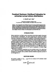
Figure 1. Plot of f (t) (solid line −), µi (broken line −−), and yi (stars ∗).

to facilitate the nonnegative constraint. We shall later refer to this modified Newton-Raphson method the positive Newton-Raphson algorithm. We choose a mixture of two normal densities as the test function f (t): f (t) =

2 2 2 2 1 1 2 1 √ e−(t−0.3) /(2×0.015 ) + √ e−(t−0.5) /(2×0.043 ) , 3 2π 0.015 3 2π 0.043

for 0 ≤ t ≤ 1. Figure 1 shows f (t) has two pronounced modes. The kernel function k(x, t) is a scaled normal density given by k(x, t) = R 1

k0 (x, t)

, k0 (x, t)dt √ 2 2 where k0 (x, t) = e−(t−x) /(2×0.045 ) /( 2π 0.045) for 0 ≤ x ≤ 1 and 0 ≤ t ≤ 1. Let tj = j/101, j = 0

0, 1, . . . , 100, then the j-th element of θ is θj = f (tj ). We also select xi = i/101 for i = 0, 1, . . . , 100, Pp then aij , the (i, j)-th element of A, is calculated by aij = k0 (xi , tj )/ k=1 k0 (xi , tk ). In this context p = 101 and A has the dimension of 101 × 101. After calculating µi = Ai θ for each i, yi are generated by adding Gaussian noise to µi (we are likely to obtain negative yi values). In order to enforce the condition of yi being nonnegative (see Section 2) we simply set negative yi values to zero. R1 The penalty function used in estimation is 12 0 f 00 (t)2 dt (roughness penalty) and the smoothing parameter is h = 10−7 . [9] demonstrate that this roughness penalty, under certain conditions, can be expressed in a quadratic form 21 θ T Rθ, where R is a particular band matrix. By defining “convergence” as the consecutive iteration changes for all θj are less then 10−3 , the MII-L algorithm converges after 886 iterations with the penalized log-likelihood value −5.8867. The positive Newton-Raphson method reaches convergence in 1 iteration and the corresponding penalized log-likelihood value is −6.2358; clearly it does not provide the correct NNMPL solution. Figure 2 displays the reconstructions and they appear differently, particularly at the turning points and the tails of the curve.

Multiplicative algorithms for MPL inversion

14

Plot of reconstructions 9

MII−L Newtons

8

7

6

5

4

3

2

1

0 0

0.1

0.2

0.3

0.4

0.5

0.6

0.7

0.8

0.9

1

Figure 2. Plot of reconstructions by MII-L (solid line −) and positive Newton-Raphson

method (broken line −−).

5.2. Emission tomography Image reconstruction from projections in medical imaging is a technique having wide applications. Particularly, emission tomography aims to estimate, from the projection data, the local photon emission intensities of a section of a patient’s body. Because of the Poisson noise in projection data (due to the physical procedure of data collection; see, for example, [29]), ML or MPL can be used to form statistical image reconstructions. Traditional optimization methods, such as Newton-Raphson or Fisher scoring, are impractical mainly because of the size of the linear system which needs to be solved at each iteration. The EM algorithm [29, 15] is very attractive for ML reconstructions, as it has a simple iterative formula and imposes the nonnegative constraints automatically. However EM iterations converge very slowly, especially at high frequency components of the reconstructed image. The EM algorithm could also be used for finding the MPL reconstruction, but its iterations are no longer simple to implement due to the penalty function. Green’s one-step-late (EM-OSL) [10] is a modification to the standard EM and it avoids the complexity introduced by the penalty function. However EM-OSL does not guarantee that all reconstructions are positive. In contrast, the MII-F and MII-L algorithms assure positivity. Following the model specification of [29] for single photon emission computed tomography (SPECT), let measurements (i.e. projection counts) y1 , . . . , yn be independent Poisson variables with Pp means µi = E(yi ) = j=1 aij θj , i = 1, . . . , n, where weights aij are assumed known, representing the mean rate of arrival at camera detector i for photons emitted from pixel j, and θj is the emission rate at pixel j. Let θ be the p × 1 vector for all θj , the MPL estimate of θ is given by maximizing the

Multiplicative algorithms for MPL inversion

15

penalized log-likelihood function n X lh (θ) = {yi log µi − µi } − hJ(θ).

(26)

i=1

The EM-OSL algorithm updates θj iteratively by Pn (k) aij yi /µi (k+1) (k) θj = θj Pn i=1 . (k) 0 )) i=1 aij + hJj (θ

(27)

The EM-OSL algorithm, in its current form, may not converge to the MPL solution. [13] modifies EM-OSL by introducing a line search step. In contrast, the MII algorithm adopts the following iterative scheme for the NNMPL reconstructions:

Pn (k+1)

θj

(k)

= θj

i=1

(k)

aij yi /µi

Pn

i=1

− h min(0, Jj0 (θ (k) ))

aij + h max(0, Jj0 (θ (k) ))

.

(28)

When h = 0 this coincides with the EM algorithm of [29] for emission tomography. When h 6= 0 the MII algorithm by itself may not be convergent; instead MII-F or MII-L assure local or global convergence. We applied the MII-L algorithm to a simulated, and simplified, SPECT image reconstruction problem. This simulation used a phantom of size 64 × 64 pixels; see picture (f) of Figure 3. This phantom represents the chest area of a human body: the two low activity circles indicate the lungs and the high activity ring corresponds to the myocardia. In the system, there were 64 projection angles and the projections rotated 3600 . There were 64 camera bins in each projection. The projection matrix A (a sparse matrix with dimension 642 × 642 ) was pre-determined by the geometry of pixels and projections with attenuation map specified. We include attenuation corrections to the elements of A so that it closely simulates a real medical imaging system. Poisson distributed projection counts were obtained in two steps: firstly, the mean values vector µ = Aθ was generated and secondly, Poisson noise was added to elements of µ. In this study the total observed projection count was 883,684 (allowing for attenuation), and the average photon emission count per pixel was 1000. We used quadratic penalty J(θ) = 12 θ T Rθ in the reconstructions with R given by: rjt = −0.25 for j 6= t and t in the first-order neighborhood of j, rjj = 1 for all j and other rjt = 0. This function penalizes discrepancies between each pixel and its four immediate (first-order) neighbors. Note for any column j of matrix A, if all entries aij are zero, then the corresponding pixel activity θj must be zero. Thus we use only those nonzero columns (i.e. at least one nonzero element in a column) of A to estimate nonzero θj ’s. By selecting the smoothing parameter h = 3 × 10−6 , we ran 2000 iterations of MII-L. With “convergence” being defined the same as in Section 5.1, MII-L did not reach convergence even after 2000 iterations; its log-likelihood value was 3, 876, 959.66 at the 200-th iteration and 3, 876, 960.57 at the 2000-th iteration. Clearly the MII-L algorithm, in this example, still endures slow convergence of the EM algorithm, particularly in the latter iterations. The MII-L reconstructions at iteration 30, 50, 100, 150 and 200 are displayed in Figure 3.

Multiplicative algorithms for MPL inversion

16

(a)

(b)

(c)

(d)

(e)

(f)

Figure 3. MII-L reconstructions at iterations (a) 30, (b) 50, (c) 100, (d) 150 and (e) 200.

The true phantom is in (f ).

6. Discussions The nonnegative constraints appear in many inverse problems, such as medical image reconstruction, picture restoration, seismic data deconvolution, etc. Due to the huge parameter dimension, how to impose the nonnegative constraints efficiently becomes a difficult question. This paper develops a multiplicative iterative algorithm that is capable of producing the NNMPL solutions when both observations and point-spread-function are nonnegative. We show that, when there is no penalty (i.e. h = 0), this algorithm converges almost surely, and when there is a penalty, (i.e. h 6= 0), either fixed relaxation or line search are necessary in order to achieve convergence. We also demonstrate, under certain conditions, that, if the algorithm converges, it will converge to the point where the Kuhn-Tucker necessary conditions for constrained optimization are satisfied. Furthermore we propose a quick penalized log-likelihood computation when line search is considered. When h = 0 and the error distribution is Poisson or Gaussian our method concurs with EM and ISRA, respectively, for medical image reconstruction from projections.

[1] S Ahn and J. A. Fessler, Globally convergent image reconstruction for emission tomography using relaxed ordered subsets algorithms, IEEE Trans. Med. Imaging 22 (2003), 613–626. [2] G. E. B. Archer and D. M. Titterington, The iterative image space reconstruction algorithm (ISRA) as an alternative to the EM algorithm for solving positive linear inverse problems, Statistica Sinica 5 (1995), 77–96. [3] N. G. Becker and I. C. Marschner, A method for estimating the age-specific relative risk of HIV infection from AIDS incidence data, Biometrika 80 (1993), 165–178. [4] C. A. Bouman and K. Sauer, A unified approach to statistical tomography using coordinate descent optimization, IEEE Trans. Med. Imaging (1996).

Multiplicative algorithms for MPL inversion

17

[5] M. E. Daube-Witherspoon and G. Muellehner, An iterative image space reconstruction algorithm suitable for volume ECT, IEEE Trans. Med. Imaging MI-5 (1986), 61–66. [6] G. D. De Villiers, B. McNally, and E. R. Pike, Positive solution to linear inverse problems, Inverse Problems 15 (1999), 615–635. [7] S. Dharanipragada and K. S. Arun, A quadratically convergent algorithm for convex-set constrained signal recovery, IEEE Trans. Sig. Proc. 44, No. 2 (1996), 248 – 266. [8] P. P. B. Eggermont, Multiplicative iterative algorithms for convex programming, J. Linear Algebra Appl. 130 (1990), 25–42. [9] P. J. Green and B. W. Silverman, Nonparametric regression and generalized linear models, Chapman and Hall, London, 1994. [10] P.J. Green, On use of the EM algorithm for penalized likelihood estimation, J. Roy. Statist. Soc. B 52 (1990), 443–452. [11] M. Hanke, J. G. Nagy, and C. Vogel, Quasi-newton approach to nonnegative image restoration, Lin. Alg. Appl. 316 (2000), 223–236. [12] J. Kirsch, An introduction to the mathematical theory of inverse problems, Springer, Berlin, 1996. [13] K. Lange, Convergence of EM image reconstruction algorithms with Gibbs smoothing, IEEE Trans. Med. Imaging MI-9 (1990), 439–446. [14] K. Lange, M. Bahn, and R. Little, A theoretical study of some maximum likelihood algorithms for emission and transmission tomography, IEEE Trans. Med. Imaging 6 (1987), 106–114. [15] K. Lange and R. Carson, EM reconstruction algorithms for emission and transmission tomography, J. Comp. Assisted Tomography 8 (1984), 306–316. [16] H. Lant´ eri, M. Roche, and C. Aime, Penalized maximum likelihood image restoration with positive constraints: multiplicative algorithms, Inverse Problems 18 (2002), 1397–1491. [17] H. Lant´ eri, M. Roche, O. Cuevas, and C. Aime, A general method to devise maximum-likelihood singal restoration multiplicative algorithms with non-negativity constraints, Signal Processing 81 (2001), 945–974. [18] L. B. Lucy, An iterative technique for the rectification of obeserved distributions, Astron. J. 79 (1974), 745–754. [19] D. Luenberger, Linear and nonlinear programming (2nd edition), J. Wiley, 1984. [20] P. McCullagh and J. A. Nelder, Generalized linear models (2nd edition), Chapman and Hall, London, 1989. [21] J. M. Mendel, Optimal seismic deconvolution, Academic Press, New York, 1983. [22] A. Mohammad-Djafari, J. F. Giovannelli, G. Demoment, and J. Idier, Regularization, maximum entropy and probabilistic methods in mass spectrometry data processing problems, International Journal of Mass Spectrometry 215 (2002), 175–193. [23] E. Mumcuoˇ glu, R. Leahy, S. R. Cherry, and Z. Zhou, Fast gradient-based methods for bayesian reconstruction of transmission and emission PET images, IEEE Trans. Med. Imaging 13 (1994), 687–701. [24] J. A. Nelder and R. W. M. Wedderburn, Generalized linear models, J. Roy. Statist. Soc. A 135 (1972), 370–384. [25] J. M. Ortega and W. C. Rheinboldt, Iterative solutions of nonlinear equations in several variables, Academic Press, New York, 1970. [26] Lee C. Potter and K. S. Arun, A dual approach to linear inverse problems with convex constraints, SIAM Journal of Control and Optimization vol. 31, no. 4 (1993), 1080–1092. [27] W. H. Richardson, Bayesian based iterative method for image restoration, J. Opt. Soc. Am. 62 (1972), 55–59. [28] F. Sha, L. K. Saul, and D. D. Lee, Multiplicative updates for nonnegative quadratic programming in support vector machines, Technical Report, University of Pennsylvania MS-CIS-02-19 (2002). [29] L. A. Shepp and Y. Vardi, Maximum likelihood estimation for emission tomography, IEEE Trans. Med. Imaging MI-1 (1982), 113–121. [30] D. L. Snyder, T. J. Schulz, and J. A. O’Sullivan, Deblurring subject to nonnegativity constraints, IEEE Trans on Signal Processing 40 (1992), 1143 – 1150.

Multiplicative algorithms for MPL inversion

18

[31] R. A. Tapia and J. R. Thompson, Nonparametric probability density estimation, The Johns Hopkins University Press, 1978. [32] T. Tikhonov and V. Arsenin, Solutions of ill-posed problems, Wiley, New York, 1977. [33] Y. Vardi and D. Lee, From image deblurring to optimal investment: maximum likelihood solutions for positive linear inverse problems, J. Roy. Statist. Soc. B 55, No. 3 (1993), 569–612. [34] Y. Vardi, L. A. Shepp, and A. Kaufman, A statistical model for positron emission tomography (with discussion), J. Amer. Statist. Assoc. 80 (1985), 8–37. [35] W. Wang, C. Goldstein, and G. Gindi, Noise and resolution properties of gamma-penalized likelihood reconstruction, Proc. IEEE Nuclear Science Symposium and Medical Imaging Conferences Vol. 2 (1998), 1136–1140. [36] D. C. Youla and H. Webb, Image restoration by the method of convex projections: part 1 - theory, IEEE Trans. Med. Imaging MI-1(2) (1982), 81–94. [37] T. S. Zaccheo and R. A. Gonsalves, Iterative maximum-likelihood estimators for positively constrained objects, J. Opt. Soc. Amer. A 13 (1996), 236–242.