Contents. 1 Introduction. 1. 2 Previous Work. 4. 3 Method. 5. 3.1 Data Representation . ... correct manual matchings are shown with white bold lines. ..... carbon Exploration and Production Series: Mathematics in Industry, vol.7, pp.89-107, ... [25] D.S. Lalush and B.M.W.Tsui, âSimulation evaluation of Gibbs prior distributions.
Bayesian based Horizon Matchings across Faults in 3d Seismic Data Fitsum Admasu and Klaus Tönnies Institute für Simulation und Graphik Otto-von-Guericke-Universität Magdeburg Postfach 4120, D-39016 Magdeburg, Germany
i
Contents 1 Introduction
1
2 Previous Work
4
3 Method 3.1 Data Representation . . . . . . 3.2 Problem Representation . . . . 3.3 Bayesian Formulation . . . . . . 3.3.1 Prior Model . . . . . . . 3.3.2 Data Model . . . . . . . 3.4 Searching for Matching Solution 3.5 Multi-resolution Model . . . . .
. . . . . . .
5 5 5 6 6 8 9 10
4 Experiments and Results 4.1 Fault Geometry Extraction . . . . . . . . . . . . . . . . . . . . . . . . . . . 4.2 Horizon Geometry Extraction . . . . . . . . . . . . . . . . . . . . . . . . . 4.3 Matching Horizons across Faults . . . . . . . . . . . . . . . . . . . . . . . .
11 11 11 12
5 Conclusions
16
Bibliography
17
. . . . . . .
. . . . . . .
. . . . . . .
. . . . . . .
. . . . . . .
. . . . . . .
. . . . . . .
. . . . . . .
. . . . . . .
. . . . . . .
. . . . . . .
. . . . . . .
. . . . . . .
. . . . . . .
. . . . . . .
. . . . . . .
. . . . . . .
. . . . . . .
. . . . . . .
. . . . . . .
. . . . . . .
. . . . . . .
. . . . . . .
ii
List of Figures 1.1 1.2
3.1 3.2
3.3
3.4 4.1
4.2 4.3
4.4
4.5
Seismic data with manually interpreted faults and horizon. . . . . . . . . . A. Pre-fault and B. Post-fault configuration of rock layers. C. Seismic slice with manually interpreted horizons curves which are cut by a fault (dashed line). Only a single slice selected from 3d seismic data is shown. . . . . . .
2
3
A. Seismic data representing a fault patch. B. Abstraction of horizons surfaces and a fault plane. . . . . . . . . . . . . . . . . . . . . . . . . . . . 6 A. Horizon should not cross each other. The middle matching pair violate this constraint. B. Fault offsets have only one direction. The middle matching pair violate this constraint. . . . . . . . . . . . . . . . . . . . . 7 A. Matched horizons with their fault throws shown on bold on the dashed fault line. B. Fault throw contours on a fault surface have ideally elliptical shapes. . . . . . . . . . . . . . . . . . . . . . . . . . . . . . . . . . . . . . 8 Horizon segments generated on the seismic slices, at different resolution level. 10 A. Seismic inline slice. B. Fault enhancing by convolving with log-Gabor filters. C. Automatically detected fault line (white line). D. A fault surface is fitted to the fault lines on sequence of seismic slices. . . . . . . . . . . A. Salient segments of horizons detected on a seismic slice. B. Interconnection of salient segments to form a horizon surface. . . . . . . . . . . . . . A. Many incorrect matchings (dark lines) due to poor data quality. The correct manual matchings are shown with white bold lines. B. Many incorrect matchings (dark lines) due to fault interaction. The correct manual matchings are shown with white bold lines. . . . . . . . . . . . . . . . . A. Horizons matching results of RJMCMC algorithm with seismic similarity. The broken ellipse region shows mismatches and omissions. B. Improved results when the prior constraints are integrated in the matching. C. Manual matchings (the differences with B) are shown with bold line. . . . . . . . . . . . . . . . . . . . . . . . . . . . . . . . . . . . . . . A. Incorrect matchings due to insufficient information on 2d seismic slices. B. Correct matchings when more slices from the same fault patch are utilized. C. Reference manual matchings (the difference with B) are shown on bold arrow. . . . . . . . . . . . . . . . . . . . . . . . . . . . . . . . .
. 12 . 12
. 13
. 14
. 14
4.6
A. Wrong matching pairs (corrected by white arrows) are obtained when all horizons are considered for matching search (i.e no multi-scale search). B. Coarse matching: few horizons selected and matched. C. Improved results using the previous results as constraints. . . . . . . . . . . . . . . . . . . . 15
iii
Abstract Oil and gas exploration decisions are made based on inferences obtained from seismic data interpretation. While 3D seismic data become widespread and the data-sets get larger, the demand for automation to speed up the seismic interpretation process is increasing as well. However, the development of intelligent tools which can do more to assist interpreters has been difficult due to low information content in seismic data. Image processing tools such as auto-trackers assist manual interpretation of horizons, seismic events representing boundaries between rock layers. Auto-trackers works to the extent of observed data continuity; they fail to track horizons in areas of discontinuities such as faults. In this paper, we present a method for automatic horizon matching across faults based on a Bayesian approach. A stochastic matching model which integrates 3d spatial information of seismic data and prior geological knowledge is introduced. The optimal matching solution is found by MAP estimate of this model. A multi-resolution simulated annealing with reversible jump Markov Chain Monte Carlo algorithm is employed to sample from aposteriori distribution. The multi-resolution is obtained in scale-space like representation using perceptual resolution of the scene. The model was applied to real 3d seismic data, and has shown to produce horizons matchings which compare well with manually obtained matching references. Further tests show that the inclusions of 3d spatial continuity and multi-resolution aspects of the dataset lead to more robust and correct results.
1
Chapter 1 Introduction Subsurface regions offering prospects for the existence of hydrocarbons undergo a seismic survey to get the profile of their underground structure. An exploration well is drilled to conclusively determine the presence or absence of oil/gas. Since drilling a well is an expensive, high-risk operation, every care should be taken and all available information needs to be exploited before arriving any exploration decision. A seismic survey consists of seismic data acquisition and interpretation. Seismic data are pictures showing subsurface seismic reflectivity. They are acquired by sending artificially created seismic wave signals from a ground surface and recording reflections from underground rock layers. The recorded seismic signal consists of amplitudes of various strength and sign (peaks or troughs). After several preprocessing steps the recorded signals are ready for interpretations. 3d seismic data consist of numerous closely-spaced seismic lines in three dimensions: seismic lines, seismic traces, and time (see figure 1.1). Each seismic line indicates the seismic shoot line and a seismic trace is the area covered by each seismic record. The area resolution ranges from 12.5 m to 25 m [9]. The time dimension is measured in TWT (Two Way Travel) time unit which is the time spent when the signals sent from the surface go down and return. Usually time sampling in 2ms is done for about 6 seconds resulting in about 3000 time slices. Structural interpretation of seismic data attempts to create 3D subsurface models and involves the interpretation of faults and horizons [5]. Faults are fractures of rock layers. They are identified by finding the reflected event termination and are usually interpreted as straight lines or connected line segments (see fault lines in figure 1.1). Horizons appear as linear structures and indicate interfaces between underground rock layers. Horizon tracking is performed by following continuity, high-amplitudes and avoiding ambiguities such as high frequencies (see figure 1.1 for interpreted horizon). The horizon interpretation task also involves jump correlation of horizons across faults (see jump correlation of horizons on figure 1.1). Human interpreters evaluate their interpretation decision on 2-d slices. The 3-d nature of the data set can be appreciated only if a sequence of slices is displayed. This is done frequently as the information from a single slice is often inconclusive.
Figure 1.1: Seismic data with manually interpreted faults and horizon. This paper research work is motivated by the demands of computer-assisted structural interpretation of seismic data. At present most parts of seismic interpretation are done manually. It takes too long to build trusted models for exploration decisions. Seismic data have sizes of several gigabytes of data containing thousands of slices. Manual structural interpreting on each seismic slice is time consuming and error prone. Further, manual interpretation results are interpreters biased and lack well specified reliability measures. Computer-assisted interpretation has the advantage of providing faster interpretation and a consistent workflow. With the work presented here, we address one of the major problems in seismic interpretation which is the matching of horizons across faults (see figure 1.2). We assume that horizon surfaces in unfaulted regions are given (e.g. by applying an autotracker [8]) and fault surfaces have been generated (e.g. by a methodology suggested by [11]). We restrict our work to normal faults which is the most common fault type where one side of the fault block (hangingwall) moves down relative to the other side (footwall). Since the two sides of the fault may have undergone different geological processes, such as compression and erosion, scale differences between horizons on the two sides can be expected and some horizons on one side may not have matches on the other side of the fault. Automating horizon matching is very challenging due to non-dense seismic information, local distortions, and large number of possible configurations.
2
Figure 1.2: A. Pre-fault and B. Post-fault configuration of rock layers. C. Seismic slice with manually interpreted horizons curves which are cut by a fault (dashed line). Only a single slice selected from 3d seismic data is shown.
3
4
Chapter 2 Previous Work The horizon matching problem can not be solved using classical stereo correspondence [17] or registration algorithms [6] due to little intensity information to guide the utilization of optical flow and presence of local distortions. Artificial neural networks [2] and gaussian clustering [4] techniques have been proposed for matching horizons across faults. However, both use only local seismic similarity measures and thus their successes are very limited. A model-based scheme for matching horizons at normal faults in 2-d seismic images is introduced in [3]. Well-defined horizons segments on both sides of the fault were extracted and matched based on local correlation of seismic intensity and geological knowledge. However, a pure 2-d approach lacks efficiency and is suitable only if the information of the 2-d seismic slice is sufficient for evaluation of the geological constraints. Another paper [1] introduces a multi-resolution continuous horizon correlation scheme where the correlation task is formulated as a non-rigid continuous point matching between the two sides of the fault. It has the advantage that it does not require all horizons to be welldefined. However, it is computational expensive and not sufficiently robust with respect to noise and artifacts in seismic data. The original contribution of this work is that we aim to exploit existing 3-d spatial relationships in the data directly for robust matching across faults. We introduce a stochastic model, which integrates data term and prior geological constraints. The data term incorporates seismic data properties through statistical measures of local homogeneities and contrast in 3d space. The a-priori geological constraints are modelled through interactions of geometric primitives. The stochastic nature of the model provides quality measures and a sampling means to find matching solutions. Further, we introduce a multi-resolution search strategy where strong horizons signals give guidance for matching weaker horizons.
5
Chapter 3 Method 3.1
Data Representation
A seismic data ready for structural interpretation can be represented as 3-d scene Sd = (V, F ), where V ⊆ R3 indicates the space covered by the seismic survey and F is a real-valued scalar field such that F : R3 → R. For c ∈ V , c = (x, y, z) denotes a position in seismic data dependant coordinate system and x, y, and z span respectively the seismic line, the seismic trace, and the time. F is a function that assigns to every voxel c seismic amplitude value F (c). The given primitives, the fault plane and the horizons surfaces, are defined in the similar scene space, Sp = (V, T ) such that T : V → L and T (c) = l, for l ∈ L = {p, Hf 1 , Hf 2 , ..., Hf m , Hh1 , Hh2 , ..., Hhn , 0} where p is a label for fault plane voxels, and for i ∈ Z + , Hf i s and Hhi s represent respectively labels for horizons surfaces voxels defined from foot- and hanging-walls blocks (see figure 3.1). The horizons labels are sorted in ascending order of their time coordinates such that 0 < Hf 1 < Hf 2 < ... < Hf m and 0 < Hh1 < Hh2 < ... < Hhn . T (c) = 0 if the voxel c does not belong any of the primitives, and indicates background.
3.2
Problem Representation
The horizon matching problem can be described as finding a set of matching pairs x = {x1 , .., xi , ..xs } (henceforth, configuration) and x ∈ X, such that each pair xi = (Hf pi , Hhqi ) with 1 ≤ pi ≤ m and 1 ≤ qi ≤ n joins horizons which would have been continuous had the fault not been present. X is the search space obtained by permutations and combinations of Hf × Hh where Hf = {Hf 1 , Hf 2 , ..., Hf m } and Hh = {Hh1 , Hh2 , ..., Hhn }. Post-fault configurations imaged by the seismic data do not provide the complete information about the pre-fault configuration of the horizons. Therefore, the geological continuity of horizons across faults are established using additional non-observed geological information. The matching problem is combinatorial with large search space, X. The size of X is
Figure 3.1: A. Seismic data representing a fault patch. B. Abstraction of horizons surfaces and a fault plane. estimated as |X| '
3.3
PN d=1
|Xd | such that |Xd | = (N d ) and N = |Hf | ∗ |Hh |.
Bayesian Formulation
We use the probability to theory to decide the most likely configuration or matching solution. Let fx represent the seismic amplitude features for a configuration x. Then the logical connection between the configuration x and the data fx are determined with P (x | fx ). Using the Bayes law, P (x | fx ) =
P (x)P (fx | x) P (fx | x)
(3.1)
In the following two sections, we describe a priori model for computing P (x) and data model for computing P (fx | x).
3.3.1
Prior Model
Consider the geometries of the horizons primitives have uniform poisson point processes, then the configuration x are from Gibbs random field (GRF) and P (x) forms a Gibbs distribution [14]: 1 n(x) ( −U (x) ) β e T (3.2) Z where U (x) is an energy evaluated by interactions of the geometric primitives, Z is normalization constant, and β stands for a scale parameter. T is the temperature of the system. No priori knowledge regarding the topology of a single horizon can be defined. However, we can impose geological constraints when dealing with a sequence of horizon layers. These constraints are described below as C1 and C2 . P (x) =
6
Figure 3.2: A. Horizon should not cross each other. The middle matching pair violate this constraint. B. Fault offsets have only one direction. The middle matching pair violate this constraint. C1 states that horizons must not cross each other, and is computed as ½ ∞, if horizoncross(x)==true C1 (x) = 0, otherwise
(3.3)
where the function horizoncross(x) checks and returns true if matched horizons result in crossing each other (see figure 3.2A). C2 states that offsets have only one direction, and is estimated as ½ 0, if consistency(x)==true (3.4) C2 (x) = ∞, otherwise where the function consistency(x) examines the offsets directions of the matched horizons and returns true if they are consistent (see figure 3.2B). Another soft geological constraint C3 is imposed using heuristically determined theoretical fault throw function. Fault throw is the vertical offset of the displaced horizons (see figure 3.3A). Fault throw is maximum at the mid of the fault surface and decreases to zero towards the tips of the fault surface. Longer faults have larger throws. The fault plane may be approximated by an elliptic shape according to [7], [22] (see figure 3.3B). Then, the fault throw value at a given point on the fault surface may be estimated by a function fd as follows: fd (r) = 2D(((1 + r)/2)2 − r2 )2 (1 − r)
(3.5)
where r is the normalized radial distance from the fault center and D is the maximum fault throw value. Horizons offsets of each matching pairs are represented with a set Dx = {d1 , d2 , ..., dN } where di represents the offsets of the joined up horizons, xi . Correspondingly, expected fault offsets Ux = {u1 , u2 , ..., uN } for the matching pairs are estimated using equation 3.5. The fault model contains unknown latent values,Θ (fault width, length, center and maximum fault throw). Considering the gaussian mixture and applying the expectation maximization algorithm, the Ux and Θmax are estimated. Then C3 = log(
N X
αj pΘmax (dj | uΘmax ))
j=1
7
(3.6)
Figure 3.3: A. Matched horizons with their fault throws shown on bold on the dashed fault line. B. Fault throw contours on a fault surface have ideally elliptical shapes. Finally the the a-priori energy, U (x), in equation 3.2 is computed as: U (x) = C1 (x) + C2 (x) + C3 (x)
3.3.2
(3.7)
Data Model
Horizons represent topological surfaces of homogenous rock layers. This homogeneity usually reflected in the seismic data as similar amplitude values. Although this similarity does not mean identical amplitudes or iso-surfaces, a characterization can be derived which capture the local strong seismic similarity expected on horizon topological surfaces. Previous implicit horizon models utilized in auto-picking tools [8] and other horizon matching algorithms [2] [4] [3] [1] do not capture any spatial variability of horizon seismic signals. Here we introduce a novel explicit modelling of 3d horizon surfaces for automation purpose. The seismic signals observed on the topological surfaces of matched horizons are modelled as gaussian random process, h(t) where t ∈ V, h(t) = F (t) and t represents the voxels of the joined horizons surfaces. Then, the gaussian process is specified by mean µ(t) = E(h(t)) and its covariance function cov(t, t0 ) = E[(h(t) − µ(t))(h(t0 ) − µ(t0 ))], t0 ∈ V . The gaussian model is selected for its flexibility and easiness to impose the priori knowledge of seismic similarity. Ignoring the offsets due to faulting, the spatial correlation of h(t) is estimated as γ(d) = E{h(t + d) − h(t)]2 }.
(3.8)
for a lag distance d. This expectation is estimated as the average squared difference of values separated by d. γ(d) '
1 X [h(t) − h(t + d)]2 N (d)
(3.9)
N (d)
where N (d) is the number of pairs for lag d. Then for a configuration, x, the likelihood probability P (h(x)) in equation 3.1 is estimated as Y P P (fx | x) ∝ e−( d γ(d)) (3.10) xi
8
3.4
Searching for Matching Solution
The optimal matching solution is the marked point set xmax = (x1 , ..., xi , ..., xs ) that maximizes P (x | h(x)) where xmax = arg max P (x | fx )
(3.11)
xmax = arg max log(P (x | fx ))
(3.12)
x
x
Using equation 3.10 and 3.2, and ignoring the normalization probability in equation 3.1 XX xmax = arg min[U (x) + ( γ(d))] (3.13) x
xi
d
This is a MAP estimation problem and xmax is searched in space X. Since X is too big for a direct search, simulated annealing with a Reverse Jump Markov Chain Monte Carlo (RJMCMC) [12] sampling method is utilized. We introduce an other random variable, S, which counts the number of matching pairs in marked set, x. That means S = |x| and is assumed to have a poisson distribution. The RJMCMC algorithm generates artificial Markov chains that transit between states of different dimension depending on the temperature (see algorithm 1). Algorithm 1: Initialize init_state = (x1 , ..xi , ..xs ) and k = 0. Hf 0 ⊆ Hf and Hh0 ⊆ Hh are set of labels such that for x = (f, h) ∈ init_state f 6= l if l ∈ Hf 0 or h 6= l for l ∈ Hh0 . While the temperature T is above the minimum temperature, do the following, 1. Step k = k + 1 and generate r ∼ U [0, 1] 2. Using r perform one of the following moves (a) Select uniformly xpf and xph respectively from Hf 0 and Hh0 and form xp = (xpf , xph ) and set new_state = init_state ∪ {xp }. (b) Select uniformly xp from the init_state and set new_state = init_state\{xp }. (c) Uniformly select xp = (xpf , xph ) from init_state and xpf new from Hf 0 set new_state = (init_state \ {xp }) ∪ {(xpf new , xph )}. (d) Uniformly select xp = (xpf , xph ) from init_state and xphnew from Hh0 set new_state = (init_state \ {xp }) ∪ {(xpf , xphnew )}. 3. Compute the ratio probability,P , let P = min{1,
p(|xnew |) p(xnew | fxnew ) } p(|xinit |) p(xinit | fxinit )
where xnew = new_state and xinit = init_state 4. Accept or reject new_state with a probability, P . 5. Decrease the temperature, and update init_state, Hf 0 and Hh0 . 9
3.5
Multi-resolution Model
As the number of horizons increases, it takes too long for Algorithm 1 to find the global optimum solution. In some cases, as the parameter for the algorithms are fine tuned to achieve a generalization, considerable horizons may left unmatched. To solve this problem we have utilized a multi-resolution version of the matching algorithm where strong horizons are matched at the coarser level and their matching solution are utilized as priori for matching at finer level weaker horizons. The notion of hierarchical representation of a signal has been used in many contexts. Approaches to multi scale representation such as wavelet analysis [24] and scale space theory [23] [21] have been introduced. Wavelet analysis are not invariant under thickness thus not suitable for modelling faulted horizons. In scale space, the signal is represented from coarse to fine levels of detail by convolving it with a Gaussian kernel whose standard deviation plays the role of scale. Scale-spaces representation theory does not use any prior knowledge about the signals, here we determine the horizons’ scales in semantic scale, i.e using a priori knowledge about the horizons’ signals. In section 3.3.2, we assume that horizons seismic features are gaussian random process with strong correlation. The semantic multi-resolution representation is understood in terms of the likelihood of the seismic features observed on the horizons topology. Then at coarser level, higher likelihoods are considered and at finer level the threshold for the likelihood goes down and more horizons topologies are considered (see Figure 3.4). Mathematically, the horizons scale space, Ω, for scale parameter t Ωf,α (., t) = {Hf i ∈ Hf |L(Vf i ) ≥ α; Vf i = {T −1 (Hf i )}}
(3.14)
where L(Vf i ) is the likelihood function and estimated as in equation 3.10.
Figure 3.4: Horizon segments generated on the seismic slices, at different resolution level. After obtaining the hierarchal representation of the horizons, Algorithm 1 starts from lower resolution level, then at higher resolution it searches with the convergence solutions reached at the lower resolution. The lower resolution solutions are utilized to imposes constraints C1 and C2 , and to initialize latent variables in the expectation maximization algorithm for estimating C3 .
10
11
Chapter 4 Experiments and Results We have conducted experiments to evaluate the matching model developed in the previous sections. The evaluation criteria is the correctness of the matching solution. A correct solution has matched pairs which correspond with manually obtained reference solution, and has no mismatched pairs. Fault regions are selected from a 3D seismic volume of shallow-offshore Nigeria. Fault patches were isolated from the seismic data, which consist of large numbers of faults and fault systems. Each isolated fault patch contains a fault surface with seismic sections on the two sides of the surface. The seismic sections were considered to be displaced only under the influence of this single fault surface. Extractions of horizons and faults geometries are not the main focus of this paper; however, since they are required for the experiments, the procedures for extraction of these geometries are described in the following subsections.
4.1
Fault Geometry Extraction
We have developed a semiautomatic method to extract 3-d fault surfaces of constant orientation. Fault features are highlighted on seismic slices by applying a set of logGabor filters [10] at different orientation and different scales. A fault line is drawn on a slice to depict the fault to be tracked. Starting from this line, a fault surface is extracted automatically by propagating and identifying the fault lines in the successive inline slices using orientation constraints and linear regression of the filter responses of log-Gabor filter. See figure 4.1.
4.2
Horizon Geometry Extraction
Horizons topological surfaces are built semiautomatically from salient features. These salient features are local maxima of seismic amplitudes and are connected to represent fragments horizons (see figure 4.2A). Then starting from some seed segments, the fragmented horizons segments are tracked in sequence of slices and merged to form layers
Figure 4.1: A. Seismic inline slice. B. Fault enhancing by convolving with log-Gabor filters. C. Automatically detected fault line (white line). D. A fault surface is fitted to the fault lines on sequence of seismic slices. of horizons surfaces. The tracking is in multi-resolution fashion, where first complete horizon segments are identified as reference. Then fragmented ones are coupled with the closest complete segments and average distances from the respective complete segments are computed. These distances used as clues to locate and merge fragmented horizon segments (see figure 4.2B).
Figure 4.2: A. Salient segments of horizons detected on a seismic slice. B. Interconnection of salient segments to form a horizon surface.
4.3
Matching Horizons across Faults
Several normal fault surface with horizons geometries are defined semi- automatically using the procedures in the previous sections. Reference matching solutions are obtained manually. The parameters for algorithm 1 are fine-tuned to the convergence using selected fault reference solution as samples of the a-posteriori distribution. A geometric temperature cooling schedule is utilized. The initial temperature is set to allow jumping from the 12
Figure 4.3: A. Many incorrect matchings (dark lines) due to poor data quality. The correct manual matchings are shown with white bold lines. B. Many incorrect matchings (dark lines) due to fault interaction. The correct manual matchings are shown with white bold lines. possible higher energy to the lowest. The final temperature is set close to zero (∼ 0.005), the rate of temperature decrement to 0.97% and the inner loop was varied from 10 to 100 depending on the number of horizons to match. These optimization parameters are related to the time and fitness of the solution and they are set with some tolerances allowing few horizons unmatched. The method was implemented in MATLAB on Pentium IV pc running windows XP. The simulated annealing process takes from 30 sec to 10 min depending on the number of horizons. Simulated annealing test runs were executed for 17 fault patches. These fault patches are different from the fault patches utilized for estimating the parameters. Results on 14 fault patches were considered acceptable with less than 20% possible matching pairs omissions compared to the reference solutions. Matching on three faults was unsuccessful because they contain mismatches. Figure 4.3 shows for two fault patches unacceptable matching results as there are many mismatches and omissions. The manual matching references are shown with bold lines. The works in [2] [4] proposes horizon matching techniques which utilizes only seismic similarity measures measures. However, figure 4.4 demonstrates the significance of of apriori knowledge. Figure 4.4A shows a seismic slice of a fault patch of size 401 × 60 × 50 pixels. The matching results shown on this slice are obtained using only the data model similarity measure. As result large mismatches and omissions are generated (see the broken ellipse region). Acceptable matching results are achieved when incorporating of the prior constraints (figure 4.4B). The method in [3] extracts discrete prominent horizon segments on 2d slices and find matches between them. The method works only if there is enough information on 2d 13
Figure 4.4: A. Horizons matching results of RJMCMC algorithm with seismic similarity. The broken ellipse region shows mismatches and omissions. B. Improved results when the prior constraints are integrated in the matching. C. Manual matchings (the differences with B) are shown with bold line.
Figure 4.5: A. Incorrect matchings due to insufficient information on 2d seismic slices. B. Correct matchings when more slices from the same fault patch are utilized. C. Reference manual matchings (the difference with B) are shown on bold arrow. seismic section and also tends to leave a large number of horizons unmatched. Figure 4.5 demonstrates the impacts of 3d information. Our previous method [1] treats the horizon matching as a non-rigid point-based image registration. An implementation of this method was able to find satisfactory correlations only for 8 fault patches out of the 17 fault patches that are used for our test here. Our new method is more robust and faster because it matches segments which have more discriminating features than points. The multi-resolution aspect of our matching algorithm explained in section 3.5 helps to recover every possible matching pair of horizons (see Figure 4.6) and reduce the simulation time considerably from minutes to seconds.
14
Figure 4.6: A. Wrong matching pairs (corrected by white arrows) are obtained when all horizons are considered for matching search (i.e no multi-scale search). B. Coarse matching: few horizons selected and matched. C. Improved results using the previous results as constraints.
15
16
Chapter 5 Conclusions Since the ultimate goal is production, good reliable and consistent measures of the interpretation are crucial. Here we have introduced a stochastic matching model which can facilitate seismic interpretations. The stochastic nature provides quality measures such as sampling from a posteriori distribution. The automatic matching results compare well with references obtained manually. Further tests show that the inclusions of 3d spatial continuity and multi-resolution aspects of the dataset lead to more robust and correct results. Though the method fails in areas of fault interactions, it helps to bring the the attention of the interpreter and saves the interpreters time as the interpreter will give more attention for such areas than spending time in routine fault regions. Further, the erroneous results could also point to the incorrect fault definition hence pointing to misinterpretations at previous stages. The model can be further extended to incorporate other fault types and well-log observations.
17
Bibliography [1] F. Admasu and K. Toennies, “A model-based approach to automatic 3d seismic horizons correlations across faults.” In Simulation und Visualisierung 2004, pp.239-250, Magdeburg, March 2004. [2] P. Alberts, M. Warner and D. Lister, “Artificial Neural Networks for Simultaneous Multi Horizon Tracking across Discontinuities,” 70th Annual International Meeting, SEG, Houston, USA, 2000. [3] M. Aurnhammer and K. Toennies, “A genetic algorithm for automated horizon correlation across faults in seismic images.” IEEE Transactions on Evolutionary Computation, vol. 9, No. 2, pp. 201-210, 2005. [4] H. Borgos, T. Skov and L. Sonneland,“ Automated Strucural Interpretaion through Classification of Seismic Horizons,” Mathematical Methods and Modelling in Hydrocarbon Exploration and Production Series: Mathematics in Industry, vol.7, pp.89-107, 2005. [5] A.Brown, Interpretation of Three-Dimensional Seismic Data, American Association of Petroleum Geologists, 5th edition, December, 1999. [6] L. Brown, “A Survey of Image Registration Techniques”, ACM Computing Surveys, Vol. 24, No. 4, pp. 325-376, 1992. [7] P.A. Cowie, R.J. Knipe and I.G. Main,“Scaling Laws for Fault and Fracture Populations - Analyses and Applications Edited ” Journal of Structural Geology special issue 2-3, Vol.18, 1996. [8] G.A. Dorn,“Modern 3D Seismic Interpretation,” The Leading Edge, Vol. 17, No. 9, pp. 1262-1273, 1998. [9] C.L. Farmer, “ Geological Modelling and Reservoir Simulation,” Mathematical Methods and Modelling in Hydrocarbon Exploration and Production Series: Mathematics in Industry, vol. 7, pp.119-212, 2005. [10] D. Field, “ Relations Between the Statistics of Natural Images and the Response Properties of Cortical Cells,” Journal of The Optical Society of America A, Vol. 4, No. 12, pp.2379-2394, December 1987.
[11] D. Gibson, M. Spann and J. Turner,“Automatic Fault Detection for 3D Seismic Data,” Proc. 7th Digital Image Computing: Techniques and Applications, pp. 821-830, Sydney, December, 2003. [12] P. Green, “ Reversible jump Markov chain Monte Carlo computation and Bayesian model determination,” Biometrica 82, vol.57, pp.97-109, 1995. [13] M. Hargrave, A. Deighan and J. Haynes, “ What Are Interpreters For? -The Impact of Faster and More Objective Interpretation Systems ”, Presentation at PESGB Geophysical Technology Conference, London, December, 2003. [14] C. Lacoste and X. Descombes and J. Zerubia, “ Point Processes for Unsupervised Line Network Extraction in Remote Sensing,” IEEE Trans. Pattern Analysis and Machine Intelligence, 27(10): pages 1568-1579, October 2005. [15] B. Nielsen, P. Mostad, J. Gjerde,“Stochastic structural modelling,” Mathematical Geology, Vol. 35, No. 8, 2003. [16] T. Randen, S. Petersen and L. Sonneland,“Automatic extraction of fault surfaces from three-dimensional seismic data,” 71th Annual International SEG meeting, Soc. Exploration Geophysics, Expanded Abstracts, pp. 551-554, 2001. [17] D. Scharstein and R. Szeliski and R. Zabih, “A taxonomy and evaluation of dense two-frame stereo correspondence algorithms.” In Proceedings of the IEEE Workshop on Stereo and Multi-Baseline Vision, Kauai, HI, Dec. 2001. [18] D. Stoyan, W.S. Kendall and J.Mecke, Stochastic Geometry and its applications, John Wiley & Sons, 1987. [19] K. Tingdahl, O. Steen, P. Meldahl and J. Ligtenberg,“Semiautomatic detection of faults in 3D seismic signals,” Society of Exploration Geophysicists, 71st Annual Meeting, Expanded Abstracts, pp. 1953-1956, San Antonio, 2001. [20] R. Twiss, and E. Moores, Structural Geology, W-H.Freeman and Company, New York, 1992. [21] T. Lindeberg, Scale-Space Theory In Computer Vision, Kluwer Academic Publishers, 1994. [22] J. Walsh and J.Watterson, “Analysis of the relationship between displacements and dimensions of faults,” Journal of Structural Geology, Vol.10, pp.239-247, 1988. [23] A. Witkin, “Scale-space filtering,” In Proceedings of the International Joint Conference on Artificial Intelligence, pp.1019-1021, 1983. [24] S. Mallat, A Wavelet Tour of Signal Processing, Academic Press, 1999. 18
[25] D.S. Lalush and B.M.W.Tsui, “Simulation evaluation of Gibbs prior distributions for use in maximum a posteriori SPECT reconstructions.” IEEE Trans. on Medical Imaging, Vol. 11, No. 2, pp. 267-275, 1992.
19