The Bayesian approach to calibration of computer experiments using emulators ..... fix λi at this value, approximating Ï(m(·)|Dsim,Ï2) by Ï(m(·)|Dsim, Ëλ, Ï2).
Bayesian Calibration of Expensive Multivariate Computer Experiments Richard D. Wilkinson University of Sheffield This chapter is concerned with how to calibrate a computer model to observational data when the model produces multivariate output and is expensive to run. The significance of considering models with long run times is that they can be run only at a limited number of different inputs, ruling out a brute-force Monte Carlo approach. Consequently, all inference must be done with a limited ensemble of model runs. In this chapter we use this ensemble to train a meta-model of the computer simulator, which we refer to as an emulator (Sacks et al. 1989). The emulator provides a probabilistic description of our beliefs about the computer model and can be used as a cheap surrogate for the simulator in the calibration process. For any input configuration not in the original ensemble of model runs, the emulator provides a probability distribution describing our uncertainty about the model’s output. The Bayesian approach to calibration of computer experiments using emulators was described by Kennedy and O’Hagan (2001). Their approach was for univariate computer models, and in this chapter we show how those methods can be extended to deal with multivariate models. We use principal component analysis to project the multivariate model output onto a lower dimensional space, and then use Gaussian processes to emulate the map from the input space to the lower dimensional space. We can then reconstruct from the subspace to the original data space. This gives a Computational Methods for Large-Scale Inverse Problems and Quantification of Uncertainity. Edited by People on Earth c 2001 John Wiley & Sons, Ltd
This is a Book Title Name of the Author/Editor c XXXX John Wiley & Sons, Ltd
way of bypassing the expensive multivariate computer model with a combination of dimension reduction and emulation in order to perform the calibration. Figure 4 shows a schematic diagram of the emulation process. The result of a probabilistic calibration is a posterior distribution over the input space which represents our uncertainty about the best value of the model input given the observational data and the computer model. It is important when calibrating to distinguish between measurement error on the data and model error in the computer simulator predictions and in Section 0.1 we describe how both can and must be included in order to produce a fair analysis. A Bayesian belief network showing the statistical aspects of the calibration process is shown in Figure 1. The layout of this chapter is as follows. In Section 0.1 we introduce the problem and describe the calibration framework. In Section 0.2 we introduce the idea of emulation and describe the principal component emulator and in Section 0.3 we give details of how to use this approach to calibrate multivariate models. To illustrate the methodology we use the University of Victoria intermediate complexity climate model, which we will calibrate to observational data collected throughout the latter half of the twentieth century. The model is introduced at the end of Section 0.1 and is returned to at the end of each subsequent section.
0.1 Calibration of computer experiments In statistics, calibration is the term used to describe the inverse process of fitting a model to data, although it is also referred to as parameter estimation or simply as inference. Here, we consider the problem in which we have a computer model of a physical system along with observations of that system. The aim is to combine the science captured by the computer model with the physical observations to learn about parameter values and initial conditions for the model. We want to incorporate 1. the computer model, m(·), 2. field observations of the physical system, Dfield , 3. any other background information. We consider each of these sources in turn. The computer model The computer model, m(·), is considered to be a map from the input space Θ, to the output space Y ⊂ Rn . The input parameters θ ∈ Θ are the calibration parameters that we wish to estimate. They may be physical constants (although care is needed when identifying model parameters with physical constants; see Section 0.1.2), context-specific constants, or tuning parameters needed to make the model perform well. These are parameters that would not need to be specified if we were doing a physical experiment. Models also often have control parameters which act
as context indicators or as switches between scenarios. For clarity, we ignore these inputs, but note that the approach presented here can be extended to deal with this case by considering the input space to be Θ × T , where T is a space of control variables. Later in the chapter we will be concerned with models which produce multivariate output, typically with values of a variable reported at spatial locations or over a range of times, or perhaps both. We could, if we chose to, introduce an index variable to the inputs in order to reduce these models to having scalar outputs, allowing us to use methods for univariate models. For example, a model predicting the temperature on a grid of locations could be considered as predicting the temperature at a single location, where that locations is specified by an index variable in the inputs. We choose not to do this here because this limits the complexity of the problem we can analyze (as well as presenting some conceptual challenges with the emulation) and because the dimension reduction techniques appear to work better when outputs are highly correlated as they usually are if the output is a spatial-temporal field. We write m(θ) for the multivariate model output run at θ, and refer to elements in the output through an index t, so that mt (θ) is the model output at location/time t. The focus in this chapter is on calibrating computer models which have long run times. A consequence of this cost will be that we will have only a limited ensemble of model runs available to us. In other words, there will be a set of N design points D = {θi : i = 1, . . . , N } for which we know the output of the model Dsim = {yi = m(θi ) : i = 1, . . . , N }; all of the information about the model will come solely from this ensemble. The question of how to choose design points D is discussed in Section 0.2.1, and we shall assume throughout that we are provided with a well designed ensemble Dsim for use in the analysis.
Field observations We assume that we have observations of the physical system, Dfield , that directly correspond to outputs from the computer model. We let ζt represent reality at t, where t is an index variable such as time or location, and assume that the field data is a measurement of reality at t with independent Gaussian error. That is Dfield (t) = ζt + ǫt
(1)
where ǫt ∼ N (µt , σt2 ). It will usually be the case that µt = 0 for all t, and often the case that we have homoscedastic errors so that σt2 = σ 2 for all t, however neither of these assumptions is necessary for the analysis. We treat model error as separate from measurement error for reasons specified in Section 0.1.2. One of the benefits of this is that ǫ then genuinely represents measurement error. As the error rate for most instrumentation is known, and will usually be reported with the measurements, we assume µt and σt are known constants throughout. If this is not the case, it is possible to learn these these parameters along with the others.
Other background information Calibration is primarily about combining the physics in the model with field observations of the system to produce estimates of parameter values. However, there will often be additional expert knowledge that has not been built into the model. Part of this knowledge will be prior information about the likely best input values, gained through previous experiments and reading the literature, and will be represented by prior distribution π(θ). The modellers may also know something about how accurately the simulator represents the system. As explained in more detail below, when calibrating a model it is important to account for any discrepancy between the model and reality. Model builders are often able to provide information about how and where the model may be wrong. They may, for example, have more confidence in some of the model outputs than others, or they may have more faith in the predictions in some contexts than in others. This information can all be built into the analysis. Ideally, information should be elicited from the experts before they observe either the ensemble of model runs or the field data, however, in practice this will often not be the case. Garthwaite et al. (2005) give an introduction to elicitation of expert beliefs.
0.1.1 Statistical calibration framework The calibration method presented here is based on the approach given by Kennedy and O’Hagan (2001) and uses the concept of a best-input (Goldstein and Rougier 2009). The approach assumes that there is a single ‘best’ value of θ, which we label ˆ such that the model run at θˆ gives the most accurate representation of the system. θ, Note that θˆ is the best value here only in the sense of most accurately representing the data according to the specified error structure, and as commented later, the value found for θˆ need not coincide with the true physical value of θ. A consequence of this assumption is that the model run at its best input is sufficient for the model in the ˆ we can not learn anything further calibration, in the sense that once we know m(θ) about reality from the simulator. A common and incorrect assumption in calibration is to assume that we observe the simulator prediction plus independent random noise. If the computer simulator is not a perfect representation of reality, this assumption is wrong and may lead to serious errors in the analysis and in future predictions. In order to relate the simulator prediction to reality we must account for the existence of model error. We can do this with an additive error term and state that reality ζ is the best simulator prediction plus a model error δ: ˆ + δ. ζ = m(θ) (2) Equations (1) and (2) completely describe the structural form assumed in the calibration. Combing the two equations gives ˆ +δ+ǫ Dfield = m(θ)
(3)
θˆ
ˆ m(θ)
Dfield
ζ
δ
ǫ
Figure 1 A Bayesian belief network showing the dependencies between the different components in the statistical model. Note that reality separates the model prediction ˆ from the observations Dfield and from the model discrepancy δ. See Pearl m(θ) (2000) for an introduction to belief networks.
where all quantities in this equation are vectors. A consequence of the best input ˆ is independent of δ allowing us to specify beliefs about each approach is that m(θ) term without reference to the other. A schematic representation of the conditional independence structure assumed for the calibration is shown in Figure 1. In later sections, distributional assumptions are discussed for all terms on the right hand side of Equation (3), but before then we briefly consider the inferential process. Calibration is the process of judging which input values are consistent with the field data, the model and any prior beliefs. The Bayesian approach to calibration is to find the posterior distribution of the best input parameter given these three sources of information; namely, we aim to find ˆ sim , Dfield, E), π(θ|D where E represents the background information, Dsim the ensemble of model runs, and Dfield the field observations. The posterior gives relative weights to all θ ∈ Θ, and represents our beliefs about the best input in the light of the available information. To calculate the posterior distribution, we use Bayes theorem to find that the posterior of θˆ is proportional to its likelihood multiplied by its prior distribution: ˆ sim , Dfield, E) ∝ π(Dsim , Dfield|θ, ˆ E)π(θ|E). ˆ π(θ|D
(4)
ˆ E), Often, the hardest part of any calibration is specification of the likelihood π(Dsim , Dfield|θ, as once we have the prior and the likelihood, finding the posterior distribution is in theory just an integral calculation. In practice, however, this will usually require careful application of a numerical integration technique such as a Markov Chain Monte Carlo (MCMC) algorithm. Once we have made distributional assumptions ˆ the structure shown in Figure 1 allows us to calculate about δ, ǫ and possibly m(θ), the likelihood function for the data.
0.1.2 Model error There are a large variety of reasons why simulators are nearly always imperfect representations of the physical system they were designed to predict. For example, modellers’ understanding of the system may be flawed, or perhaps not all physical processes were included in the analysis, or perhaps there are numerical inaccuracies in the solver used on the underlying model equations, and so on. If we wish to make accurate predictions it is important to account for this error, as otherwise we may have an unrealistic level of confidence in our predictions. If we choose not to use a model error term we make the assumption that observations are the best simulator prediction plus white noise, i.e., ˆ +ǫ Dfield = m(θ) where ǫt is independent of ǫs for t 6= s. It will often be found that the magnitude of the measurement error associated with the measurement instrument is insufficient to account for the variability observed in the system, leading to poor model fit in the calibration. One solution might be to inflate the error variance to account for this missing variability, however, this will also cause problems with the confidence level in the predictions. In contrast to the white error structure of ǫ, the model error term δ will usually have a much richer structure, usually with δt highly correlated with δs for t close to s. By using correlated errors a better degree of accuracy can be achieved. A consequence of using an imperfect simulator in the calibration, is that model parameters may not correspond to their physical namesakes. For example, in a simulator of ocean circulation we may have a parameter called viscosity and it may be possible to conduct an experiment to measure the physical value of the viscosity in a laboratory. However, because the simulator is an imperfect representation of the system, we may find that using the physical value of the viscosity leads to poorer predictions than when using a value determined by a statistical calibration. For this reason, careful thought needs to be taken when considering which parameters to include in the calibration. The fact that model parameters may not be physical parameters should be strongly stressed to the experts when eliciting the prior distriˆ bution π(θ|E) required in Equation (4). The question of how to choose a suitable model for δ is an area of active statistical research, and the approach taken depends on the amount of data available. In situations where data is plentiful, data driven approaches can be used with an uninformative prior specification for δ. So for example, in weather prediction, each day a forecast is made and the following day data is collected which can be used to validate the previous days prediction. In situations such as this Kennedy and O’Hagan (2001) suggest the use of a Gaussian process for δ, with uninformative priors on any parameters in δ. If the data available is limited, then expert judgement becomes important. Goldstein and Rougier (2009) introduce the idea of a reified model in a thought experiment designed to help elicit beliefs about the model error. The reified model is the
version of the model we would run if we had unlimited computing resources. So for example, in global climate models the earth’s surface is split into a grid of cells and the computation assumes each cell is homogeneous. If infinite computing resources were available we could let the grid size tend to zero, giving a continuum of points across the globe. While clearly an impossibility, thinking about the reified model helps us to break down the model error into more manageable chunks; we can consider the difference between the actual computer model and the reified model, and then the difference between the reified model and reality. This approach may provide a way to help the modellers think more carefully about δ(·). Murphy et al. (2007) take a different approach and use an ensemble of models. They look at the calibrated predictions from a collection of different climate models and use these to assess what the model error might be for their model.
0.1.3 Code uncertainty If the computer model is quick to run, then we can essentially assume that its value is known for all possible input configurations, as in any inference procedure we can simply evaluate the model whenever its value is needed. In this case, calculation of the calibration posterior π(θ|Dfield , m, E) ∝ π(Dfield , |θ, m, E)π(θ|E),
(5)
where m represents the computer model, is relatively easy as the calibration framework (3) gives that ˆ = δ + ǫ. Dfield − m(θ) Given distributions for the model discrepancy δ and measurement error ǫ we can calculate the likelihood of the field data, and thus can find the posterior distribution. If the model is not quick running, then the model’s value is unknown at all input values other than those in design D. This uncertainty about the model output at untried input configurations is commonly called code uncertainty. If we want to account for this source of uncertainty in the calibration then we need a statistical model that describes our beliefs about the output for all possible input values. We introduce the idea of emulation after the following example. Example 0.1.1 (UVic Climate Model) In order to demonstrate the methodology we introduce an example from climate science which we present along with the theory. We use the University of Victoria Earth System Climate Model (UVic ESCM) coupled with a dynamic vegetation and terrestrial carbon cycle and an inorganic ocean carbon cycle (Meissner et al. 2003). The model was built in order to study potential feedbacks in the terrestrial carbon cycle and to see how these affect future climate predictions. We present a simplified analysis here, with full details available in Ricciuto et al. We consider the model to have just two inputs, Q10 and Kc , and to output a time-series of atmospheric CO2 values. Input Q10 controls the temperature dependence of respiration and can be considered as controlling a carbon source, whereas
360 340 320
CO2 level
300 1800
1850
1900
1950
2000
Year
Figure 2 Ensemble of 47 model runs of the UVic climate model for a design on two inputs Q10 and Kc . The output (black lines) gives the atmospheric CO2 predictions for 1800-1999, and the 57 field observations are shown as circles with error bars of two standard deviations.
Kc is the Michaelis–Menton constant for CO2 and controls the sensitivity of photosynthesis and can be considered to control a carbon sink. The aim is calibrate these two parameters to the Keeling and Whorf (2005) sequence of atmospheric carbon dioxide measurements. Each model run takes approximately two weeks of computer time and we have an ensemble of 47 model runs with which to perform the analysis. The model output and the field observations are shown in Figure 2.
0.2 Principal component emulation 0.2.1 Emulation If the simulator, m(·), is expensive to evaluate, then its value is unknown at all input values except those in a small ensemble of model runs. We assume that the code has been run N times for all inputs in a space-filling design D = {θi ∈ Θ : i = 1, . . . , N } to produce output Dsim = {m(θi ) ∈ Rn : i = 1, . . . , N }, and that further model runs are not available. The importance of the design D for computer experiments has been stressed by many authors (Morris and Mitchell 1995; Sacks et al. 1989) and there are numerous strategies available. A common aim is to find a space filling design that both sufficiently spans the input space and that does so in a way so that any possible θ in the input space will not be too far from a point in the design. Popular space filling designs include maximin Latin-hypercubes (Morris
and Mitchell 1995) which maximize the minimum distance between points spreading them as far as possible, and low discrepancy sequences such as Sobol sequences (Morokoff and Caflisch 1994), which have an advantage over Latin-hypercubes of being generated sequentially so that extra points can be added as required. For the purpose of emulation, a Monte Carlo sample from the input space will nearly always perform more poorly than a carefully selected design of the same size. For any θ 6∈ D we are uncertain about the value of the simulator for this input. However, if we believe that the model is a smooth continuous function of the inputs, then we can learn about m(θ) by looking at ensemble members with inputs close to θ. We could, for example, choose to predict m(θ) by linearly interpolating from the closest ensemble members. The function used to interpolate and extrapolate Dsim to other input values is commonly called an emulator, and there is extensive literature on emulation (sometimes called meta-modelling) for computer experiments (see Santner et al. (2003) for references). We use a Bayesian approach to build an emulator which captures our beliefs about the model. We can elicit prior distributions about the shape of the function, e.g., do we expect linear, quadratic or sinusoidal output, and about the smoothness and variation of the output, e.g., over what kind of length scales do we expect the function to vary. A convenient and flexible semi-parametric family that is widely used to build emulators are Gaussian processes (Stein 1999). We say f (·) is a Gaussian process with mean function g(·) and covariance function c(·, ·) and write f (·) ∼ GP (g(·), c(·, ·)) if for any collection of inputs (x1 , . . . , xn ) the vector (f (x1 ), . . . , f (xn )) has a multivariate Gaussian distribution with mean (g(x1 ), . . . , g(xn )) and covariance matrix Σ where Σij = c(xi , xj ). Gaussian process emulators can be used to predict the simulator’s value at any input, giving predictions in the form of Gaussian probability distributions over the output space. They can incorporate prior beliefs about both the prior mean structure and the covariance structure, both of which affect the behaviour when interpolating and extrapolating from design points. They are a popular alternative to the use of neural networks (Rasmussen and Williams 2006) because they include with any estimate a measure of confidence in that prediction. The conditioning to update from the prior process to the posterior process after observing the ensemble of model runs is possible analytically, and both the prior and posterior process are simple to simulate from. For univariate computer models we write m(·)|β, λ, σ 2 ∼ GP (g(·), σ 2 c(·, ·)) where g(θ) = β T h(θ) is a prior mean function which is usually taken to be a linear combination of a set of regressor functions, h(·), and where β represents a vector of coefficients. The prior variance is assumed here to be stationary across the input range and is written as the product of a prior at-a-point variance σ 2 = Var(m(θ)), and a correlation function Corr(m(θ1 ), m(θ2 )) = c(θ1 , θ2 ). Common choices for the correlation function include the Mat´ern function and the exponential correlation functions (Abrahamsen 1997), such as the commonly used squared exponential family � � c(θ1 , θ2 ) = exp −(θ1 − θ2 )T Λ(θ1 − θ2 ) . (6)
Here, Λ = diag(λ1 , . . . , λn ) is a diagonal matrix containing the roughness parameters. The λi represent how quickly we believe the output varies as a function of the input, and can be thought of as a measure of the roughness of the function. Once we observe the ensemble of model runs Dsim , we update the prior beliefs to find the posterior distribution. If we choose a conjugate prior distribution for β such as an uninformative improper distribution π(β) ∝ 1, or a Gaussian distribution, then we can integrate out β to find the posterior
m(·)|Dsim , λ, σ 2 ∼ GP (g ∗ (·), σ 2 c∗ (·, ·))
for modified functions g ∗ (·) and c∗ (·, ·). Modified function g ∗ and c∗ are the updated mean and covariance function of the Gaussian process after conditioning on observing the ensemble Dsim . Expressions for g ∗ and c∗ are given later by Equations (7) and (8) and details of the calculation can be found in Rasmussen and Williams (2006) and many other texts. It is not possible to find a conjugate prior distribution for the roughness parameters, so we take an empirical Bayes approach (Casella 1985) and give each λi a prior distribution and then find its maximum a posteriori value and ˆ σ 2 ). If we fix λi at this value, approximating π(m(·)|Dsim , σ 2 ) by π(m(·)|Dsim , λ, 2 give σ an inverse chi-squared distribution it is possible to integrate it out analytically, however, this leads to a t-process distribution for m(·) which is inconvenient later, and so we leave σ 2 and use MCMC to integrate it out numerically later in the analysis. An example of how a simple univariate Gaussian process can be used as an emulator is shown in Figure 3. The Gaussian process emulator approach described above is for univariate models. For multivariate outputs we could build separate independent emulators for each output, although this ignores the correlations between the outputs and will generally perform poorly if the size of the ensemble is small (as we are throwing away valuable information). Conti and O’Hagan (2007) provide an extension of the above approach which allows us to model a small number of multivariate outputs capturing the correlations between them, and Rougier (2008) describes an outer product emulator which factorizes the covariance matrix in a way that allows computational efficiency and so can be used on a larger number of dimensions if we are prepared to make some fairly general assumptions about the form of the regressors and the correlations. Both of these approaches require careful thought about what correlations are expected between output dimensions. This can be difficult to think about, especially with modellers who may not have much experience with either probability or statistics. Both methods are also limited by the size of problem that can be tackled, although Rougier (2008) made advances on this front. For models with hundreds or thousands of outputs a direct emulation approach may not be feasible, and so here we use a data reduction method to reduce the size of the problem to something more manageable.
8 6 4 −2
0
2
m(θ)
4 2 −2
0
m(θ)
6
8
10
Conditioned Gaussian process
10
Unconditioned Gaussian process
0
2
4
6
θ
8
10
0
2
4
6
8
10
θ
Figure 3 The left hand plots shows random draws from a Gaussian process with constant mean function (g(θ) = c for all θ) and covariance function given by Equation (6). These are realizations from the our prior belief about the model behaviour. The right hand plot shows draws from the Gaussian process after having conditioned on four data points (shown as solid black points), i.e., draws from our posterior belief about m(·). The posterior mean of the Gaussian process g ∗ (·) is shown as a thick solid line. Note that at the data points, there is no uncertainty about the value of the process.
m(·)
Θ
η pc (·)
PCA
Y
PCA−1
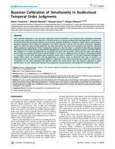
Y pc Figure 4 Schematic plot of the idea behind principal component emulation. Θ is the input space, Y the output space, and m(·) the computer model. We let η pc (·) denote the Gaussian process emulator from Θ to principal subspace Y pc .
0.2.2 Principal component emulation We take an approach here similar to Higdon et al. (2008), and use a dimension reduction technique to project the output from the computer model onto a subspace with a smaller number of dimensions and then build emulators of the map from the input space to the reduced output space. The only requirement of the dimension reduction is that there is a method for reconstruction to the original output space. We use principal component analysis here (also known as the method of empirical orthogonal functions), as the projection is then guaranteed to be the optimal linear projection, in terms of minimizing the average reconstruction error, although we could use any other dimension reduction technique as long as there is a method of reconstruction. A schematic plot of this idea is shown in Figure 4. The computer model m(·) is a function from input space Θ to output space Y. Principal component analysis provides a map from full output space Y to reduced space Y pc . We build Gaussian process emulators to map from Θ to Y pc and then use the inverse of the original projection (also a linear projection) to move from Y pc to Y. This gives a computationally cheap map from the input space Θ to the output space Y which does not use the model m(·). This cheap surrogate, or emulator, approximately interpolates all the points in the ensemble (it is approximate due to the error in the principal component reconstruction) and gives probability distributions for the model output for any value of the input. Principal component analysis is a linear projection of the data onto a lower dimensional subspace (the principal subspace) such that the variance of the projected data is maximized. It is commonly done via an eigenvalue decomposition of the correlation matrix, but for reasons of computational efficiency, we will use a singular value decomposition of the data here. Let Y denote an N × n matrix with row i the ith run of the computer model, Yi· = m(θi ) (recall that the model output is n dimensional and that there are N runs in the ensemble Dsim ). The dimension
reduction algorithm can then be described as follows: 1. Centre the matrix. Let µ denote the row vector of column means, let Y ′ be the matrix Y with µ subtracted from each row (Y ′ = Y − µ) so that the mean of each column of Y ′ is zero. We might also choose to scale the matrix, so that the variance of each column is one. 2. Calculate the singular value decomposition Y ′ = U ΓV ∗ . V is an n × n unitary matrix containing the principal components (the eigenvectors) and V ∗ denotes its complex conjugate transpose. Γ is an N × n diagonal matrix containing the principal values (the eigenvalues) and is ordered so that the magnitude of the diagonal entries decreases across the matrix. U is an N × N matrix containing the left singular values. 3. Decide on the dimension of the principal subspace, n∗ say (n∗ < n). An orthonormal basis for the principal subspace is then given by the first n∗ columns of V (the leading n∗ eigenvectors) which we denote as V1 (an n × n∗ matrix). Let V2 denote the matrix containing the remaining columns of V . 4. Project Y ′ onto the principal subspace. The coordinates in the subspace (the factor scores) are found by projecting onto V1 : Y pc = Y ′ V1 . The ith row of Y pc then denotes the coordinate of the ith ensemble member in the space Y pc . Some comments: • Note that the principal component analysis is done across the columns of the matrix rather than across the rows as is usual. The result is that the eigenvalues are of the same dimension as the original output with the leading eigenvalue often taking the general form of the output. • Although principal component analysis (PCA) is a linear projection, this method can be used on highly non-linear models. The linear aspect of PCA is the projection of the output space Y onto a smaller output space Y pc . The map from the input space Θ to the reduced output Y pc can still be non-linear, and will be unaffected by any linear assumption used in the dimension reduction. The main requirement for the use of this method, is that there is a consistent covariance structure amongst the outputs. The projection on to the principal components is essentially assuming that the true number of degrees of freedom is less than n. If the outputs are all independent then PCA will not work as a dimension reduction technique.
• There is no established method for deciding on the dimension n∗ of the principal subspace. The percentage of variance explained (sum of the corresponding eigenvalues in Γ) is often used as a heuristic, with the stated aim being to explain 95% or 99% of the variance. We must also decide which components to include in V1 . It may be found that components which only explain a small amount of the variance (small eigenvalues) are important predictively, as was found in principal component regression (Jolliffe 2002). One method of component selection is through the use of diagnostic plots as explained below. This leaves us with the coordinates of the ensemble in the principal subspace Y pc , with each row corresponding to the same row in the original design D. Gaussian processes can now be used to emulate this map. Usually, we will have n∗ > 1, and so we still need to use a multivariate emulator such as that proposed by Rougier (2008). However, emulating the reduced map with n∗ independent Gaussian processes often performs as well as using a fully multivariate emulator, especially if the size of the ensemble N is large compared with n∗ . Another computational aid that helps with the emulation is to scale the matrix of scores so that each column has variance one. This helps with tuning the MCMC sampler for the σ 2 parameters in the Gaussian process covariance function, as it makes the n∗ dimensions comparable with each other. To reconstruct from the subspace Y pc to the full space Y is also a linear transformation. We can post-multiply the scores by V1T to give a deterministic reconstruction Y ′′ = Y pc V1T . However, this does not account for the fact that by projecting into a n∗ -dimensional subspace, we have discarded information in the dimension reduction. To account for this lost information we add random multiples of the eigenvectors which describe the discarded dimensions, namely V2 . We model these random multiples as zero-mean Gaussian distributions with variances corresponding to the relevant eigenvalues. This gives a stochastic rather than a deterministic reconstruction, which accounts for the error in the dimension reduction. In summary, we reconstruct as Y ′′ = Y pc V1T + ΦV2T where Φ is an N × (n − n∗ ) matrix with ith column containing N draws from a N (0, Γn∗ +i,n∗ +i ) distribution. We then must add the column means of Y to each row of Y ′′ to complete the emulator. A useful diagnostic tool when building emulators are leave-one-out cross validation plots. These are obtained by holding back one of the N training runs in the ensemble, training the emulator with the remaining N − 1 runs, and then predicting the held back values. Plotting the predicted values, with 95% credibility intervals, against the true values for each output dimension gives valuable feedback on how the emulator is performing and allows us to validate the emulator. These plots can be used to choose the dimension of the principal subspace and which components to include. They are also useful for choosing which regressor functions to use in the specification of the mean structure. Once we have validated the emulator, we can then proceed to use it to calibrate the model.
315
325
335
True value
325
340
355
True value
350
370
400
Predicted value
1999 CO2
360
380 360
Predicted value
1987 CO2
340
Predicted value
1972 CO2 325 335 345 355
335 325 315
Predicted value
1960 CO2
390
True value
360
390
420
True value
Figure 5 Leave-one-out cross validation plots for a selection of four of the 200 outputs. The error bars show 95% credibility intervals on the predictions. The two outliers seen in each plots are for model runs with inputs on the edge of the design. These points are predictions where we extrapolate rather than interpolate from the other model runs. Example 0.2.1 (UVic continued) We use principal component emulation to build a cheap surrogate for the UVic climate model introduced earlier. Recall that the output of the model is a time-series of 200 atmospheric CO2 predictions. Figure 5 shows the leave-one-out cross-validation plots for a selection of four of the 200 output points. The emulation was done by projecting the time-series onto a 10-dimensional principal subspace and then emulating each map with independent Gaussian processes before reconstructing the data back up to the original space of 200 values. A quadratic prior mean structure was used, h(θ1 , θ2 ) = (1, θ1 , θ2 , θ12 , θ22 , θ1 θ2 )T , as the cross-validation plots showed that this gave superior performance over a linear or constant mean structure, with only negligible further gains possible by including higher order terms. The plots show that the emulator is accurately able to predict the held back runs and that the uncertainty in our predictions (shown by the 95% credibility intervals) provide a reasonable measure of our uncertainty (with 91% coverage on average).
0.3 Multivariate calibration Recall that our aim is to find the distribution of θˆ given the observations and the model runs, namely ˆ field , Dsim ) ∝ π(Dfield |Dsim , θ)π( ˆ θ|D ˆ sim ) π(θ|D ˆ θ) ˆ ∝ π(Dfield |Dsim , θ)π( ˆ = π(Dsim ) and so can be ignored in the poswhere we have noted that π(Dsim |θ) ˆ ˆ to be specified in order to find the terior distribution of θ, leaving π(Dfield |Dsim , θ) posterior. The calibration framework given by Equation (3) contains three different ˆ δ and ǫ, which we need to model. The best input approach ensures that terms, m(θ),
ˆ and δ independent for all t (Kennedy parameter θˆ is chosen so as to make m(θ) and O’Hagan 2001), and the measurement error ǫ is also independent of both terms. This allows us to specify the distribution of each part of Equation (3) in turn, and then calculate the distribution of the sum of the three components. If all three parts have a Gaussian distribution, the sum will also be Gaussian. Distributional choices for ǫ and δ will be specific to each individual problem, but often measurement errors are assumed to be zero-mean Gaussian random variables, usually with variances reported with the data. Kennedy and O’Hagan recommend the use of Gaussian process priors for the discrepancy function δ. While this is convenient mathematically, sensible forms for the discrepancy will need to be decided with the modellers in each case separately. If some non-Gaussian form is used then there may be difficulty calculating the likelihood in Equation (5). For ease of exposition, we assume δ has a Gaussian process distribution here. ˆ t) using the principal component Finally, we must find the distribution of m(θ, emulator. Before considering the map from Θ to Y, we must first consider the distribution of the emulator η pc (·) from Θ to Y pc . Using independent Gaussian processes to model the map from the input space to each dimension of the principal subspace (i.e., η pc = (η1pc , . . . , ηnpc∗ )), we have that the prior distribution for ηipc (·) is ηipc (·)|βi , σi2 , λi ∼ GP (gi (·), σi2 ci (·, ·)). If we give βi a uniform improper prior π(βi ) ∝ 1, we can then condition on Dsim and integrate out βi to find ηipc (·)|Dsim , σi2 , λi ∼ GP (gi∗ (·), σi2 c∗i (·, ·)) where ˆ gi∗ (θ) = βˆT h(θ) + t(θ)T A−1 (Y·ipc − H β)
(7)
c∗i (θ, θ′ ) = c(θ, θ′ ) − t(θ)T A−1 t(θ′ ) + (h(θ)T − t(θ)T A−1 H)(H T A−1 H)−1 × (h(θ′ )T − t(θ′ )T A−1 H)T
(8)
and βˆi = (H T A−1 H)−1 H T A−1 Y·ipc t(θ) = (c(θ, θ1 ), . . . , c(θ, θN )) {Ai }jk = {ci (θj , θk )}j,k=1,...,N H T = (h(θ1 ), . . . , h(θN )) assuming the regressors, h(·), are the same for each dimension. Here, Y·ipc denotes the ith column of matrix Y pc , and θ1 , . . . , θN are the points in design D. The reconstruction to the full space, η e (·) = η pc (·)V1T + ΦV2T , then has posterior distribution η e (θ)|Dsim , σ 2 , λ ∼ N (g ∗ (θ)V1T , σ 2 c∗ (θ, θ)V1 V1T + V2 Γ′ V2T )
where g ∗ = (g1∗ , . . . , gn∗ ∗ ) and Γ′ = diag(Γn∗ +1,n∗ +1 , . . . , Γn,n ). An empirical Bayes approach can be used for the roughness parameters by fixing them at their maximum likelihood estimates. We do not integrate σ 2 out analytically for reasons of tractability, but leave them in the calculation and use MCMC to integrate them out numerically later. If all three parts of Equation (3) are Gaussian then we can write down the likelihood of the field data conditional on the parameters: π(Dfield |Dsim , σ 2 , θ, γδ ) where γδ are parameters required for the discrepancy term δ(t). We elicit prior distributions for θ and γδ from the modellers and decide upon priors for σ 2 ourselves (emulators parameters are the responsibility of the person performing the emulation). We then use a Markov Chain Monte Carlo algorithm to find the posterior distributions. It is possible to write down a Metropolis-within-Gibbs algorithm to speed up the MCMC calculations, although we do not give the details here. Example 0.3.1 (UVic continued) Figure 6 shows the marginal posterior distributions from calibrating the UVic model to the Keeling and Whorf (2005) observations. We use an autoregressive process of order one for the discrepancy term with δt = ρδt−1 + U where U ∼ N (0, σδ2 ). We give ρ a Γ(5, 1) prior truncated at one, and σδ2 a Γ(4, 0.6) prior distribution. The Markov chains were run for 1,000,000 iterations. The first 200,000 samples were discarded as burn-in and the remaining samples were thinned to every tenth value leaving 80,000 samples. Uniform prior distributions were used for Q10 and Kc (Q10 ∼ U [1, 4] and Kc ∼ U [0.25, 1.75]), and Γ(1.5, 6) priors were used for each of the emulator variances σ 2 . Tests were done to check the sensitivity of the results to choice of prior distribution, and the analysis was robust to changes in priors for σ 2 and γδ , but not to changes in the priors for Q10 and Kc . This will not usually be the end of the calibration process. The results will be returned to the modellers, who may decide to use them to improve the model, before another calibration is performed. For details of this problem, and of the Metropoliswithin-Gibbs algorithm, see Ricciuto et al.
0.4 Summary In this chapter we have shown how to extend the calibration approach of Kennedy and O’Hagan (2001) to enable the calibration of computer models with multivariate outputs. The approach is based around the idea of emulating a reduced dimension version of the model, thus bypassing the need to repeatedly simulate from an expensive model. The method requires a well-designed ensemble of model evaluations Dsim , measurements of the system Dfield , and expert beliefs about the measurement error ǫ and possibly also the model error δ. The method can then be broken down into three steps.
1.0
1.5 4.0
0.5
2.0 1.0
0.69
3.0
Q10
0.5
1.0
1.5
Kc
1.0
2.0
3.0
4.0
Figure 6 Marginal posterior distributions for two of the calibration parameters, Q10 and Kc , in the UVic climate model. The two plots on the leading diagonal show the individual marginal plots. The bottom left plot shows the pairwise marginal distribution, and the top right box shows the posterior correlation between Q10 and Kc .
The first step is to build a cheap surrogate for the simulator to use in its place. We project the output from the true model onto a lower dimensional set of basis vectors using principal component analysis, before training Gaussian process emulators to map from the inputs to this new space. We then reconstruct to the original output space by using the inverse projection and account for data loss by using Gaussian multiples of the discarded basis vectors. The second stage is the specification of distributions in accordance with the conditional independence structure shown in Figure 1, with prior distributions needed for the calibration and error parameters. Decisions about how to model δ need to be based on each specific simulator, but Gaussian processes are a flexible form that have been found to be useful in previous applications. Finally, we must perform the inference using a Monte Carlo technique such as Markov chain Monte Carlo. This calibration methodology takes account of measurement error, code uncertainty, reconstruction error and model discrepancy, giving posterior distributions which incorporate expert knowledge as well as the model runs and field data. The limitations of this method are primarily the limitations of the Gaussian process emulator technology. The use of a dimension reduction technique requires that the outputs are correlated (as they usually are in spatial-temporal fields) and some simulators will not be represented adequately in a lower dimensional space, but this will be detected when looking at the reconstruction error. Another potential limitation is that emulators are built on the premise that m(x + h) will be close to m(x) for small h. If this is not the case, as in chaotic systems, then emulators cannot be used. For such simulators, there is no alternative to repeatedly evaluating the model. Gaussian process emulators are also limited by the size of the ensemble they can handle, due to numerical instabilities in the inversion of the covariance matrix, although methods are being developed to improve this (Furrer et al. 2006). There exists a range of validation and diagnostic tools (Bastos and O’Hagan 2009) designed to detect and correct problems in emulators, and some form of validation should always be done when using emulators. Finally, it should be stressed that the resulting posteriors do not necessarily give estimates of the true value of physical parameters, but rather give values which lead the model to best explain the data. In order to estimate the true physical value of parameters, the model discrepancy δ must be very carefully specified. This is still a new area of research and much remains to be done in the area of modelling discrepancy functions.
Bibliography Abrahamsen P 1997 A review of Gaussian random fields and correlation functions. Technical Report 917, Norwegian Computing Center, Oslo. Bastos LS and O’Hagan A (2009) Diagnostics for Gaussian process emulators. Technometrics, to appear. Box GEP 1976 Science and statistics. Journal of the American Statistical Association, 71, 791–799. Casella G 1985 An introduction to empirical Bayes data analysis. American Statistician,39(2): 83–87. Conti S and O’Hagan A 2007 Bayesian emulation of complex multi-output and dynamic computer models. In submission. Available as Research Report No. 569/07, Department of Probability and Statistics, University of Sheffield. Furrer R, Genton M G and Nychka D (2006) Covariance tapering for interpolation of large spatial datasets. Journal of Computational and Graphical Statistics 15(3), 502–523. Garthwaite PH, Kadane JB and O’Hagan A 2005 Statistical methods for eliciting probability distributions. Journal of the American Statistical Association 100, 680–701. Goldstein M and Rougier JC 2009 Reified Bayesian modelling and inference for physical systems, with discussion and rejoinder. Journal of Statistical Planning and Inference 139(3), 1221-1239. Higdon D, Gattiker J, Williams B and Rightley M 2008 Computer model calibration using high-dimensional output. Journal of the American Statistical Association 103, 570-583. Jolliffe IT 2002 Principal Component Analysis 2nd edn. Springer. Keeling CD and Whorf TP 2005 Atmospheric CO2 records from sites in the SIO air sampling network. In Trends: A Compendium of Data on Global Change, Carbon Dioxide Information Analysis Center, Oak Ridge National Laboratory, U.S. Department of Energy, Tenn., U.S.A. Kennedy M and O’Hagan A 2001 Bayesian calibration of computer models (with discussion). Journal of the Royal Statistical Society, Series B 63, 425–464. Morokoff WJ and Caflisch RE 1994 Quasi-random sequences and their discrepancies. SIAM J. Sci. Comput 15, 1251–1279. Meissner KJ, Weaver AJ, Matthews HD and Cox PM 2003 The role of land surface dynamics in glacial inception: a study with the UVic Earth System Model. Climate Dynamics 21, 515–537. Morris MD and Mitchell TJ 1995 Exploratory designs for computational experiments. Journal of Statistical Planning and Inference 43, 161–174.
Murphy JM, Booth BBB, Collins M, Harris GR, Sexton DMH and Webb MJ 2007 A methodology for probabilitic predictions of regional climate change from perturbed physics ensembles. Philosophical Transactions of the Royal Society A 365 1993–2028. Pearl J 2000 Causality: Models, Reasoning, and Inference, Cambridge University Press. Rasmussen CE and Williams CKI 2006 Gaussian Processes for Machine Learning, MIT Press. Ricciuto DM, Tonkonojenkov R, Urban N, Wilkinson RD, Matthews D, Davis KJ and Keller K Assimilation of oceanic, atmospheric, and ice-core observations into an Earth system model of intermediate complexity. In submission. Rougier JC 2008 Efficient Emulators for Multivariate Deterministic Functions. Journal of Computational and Graphical Statistics 17(4), 827-843. Sacks J, Welch WJ, Mitchell TJ and Wynn HP 1989 Design and analysis of computer experiments. Statistical Science 4, 409–423. Sacks J, Schiller SB and Welch WJ 1989 Designs for computer experiments. Technometrics, 31, 41–47. Santner TJ, Williams BJ and Notz W 2003 The Design and Analysis of Computer Experiments, Springer. Stein ML 1999 Statistical Interpolation of Spatial Data: Some Theory for Kriging, Springer.