Multivariate Calibration of Single Regime Speed-Flow-Density Relationships. Michel Van ... consistent with most multi-regime models, without the need to deal.
Multivariate Calibration of Single Regime Speed-Flow-Density Relationships Michel Van Aerde and Hesham Rakha Department of Civil Engineering, Ellis Hall, Queen’s University, Kingston, Ontario, Canada K7L 3N6
ABSTRACT This paper presents a multivariate procedure for performing automated fitting of speed-flow relationships for different roads based on loop detector data. The procedure is shown to fit the observations for different freeway, tunnel and arterial data, thus demonstrating its flexibility in terms of representing different types of roads. Furthermore, the procedure also provides a fit that is reasonable all data regimes, unlike many other single regime models that only fit free-flow or forced flow conditions data. Finally, this single-regime model provides a quality of fit that is consistent with most multi-regime models, without the need to deal with the complexities associated with the selection of regime break points. In addition to demonstrating the fit of the model to well known sample data from a standard traffic flow text books, fits to three different recent data sets with 1 to 5 minute loop detector data are also presented. These fits demonstrate that the flexibility of the proposed technique to deal with real-time data for both Europe and North America.
I. INTRODUCTION The shape of the speed-flow-density relationship of a highway facility has traditionally had a significant impact on the highway design and planning process, as the relationship would provide quantitative estimates of the change in speed as a function of anticipated or projected changes in traffic demand. Those who model or simulate highways have also experienced a similar dependence of their models on a curve that describes the sensitivity of speed or travel time to the level of traffic flow. More recently, those who desire to subject a highway to various forms of real-time control or incident detection have once again revisited the topic of calibrating speed-flow relationships. Current real-time applications of speed-flow-density relationships involve a greater dependence on the accuracy of the estimates and have a need to auto-calibrate these relationships on-line, rather than being granted the luxury to explore alternative fits off-line. A. Objectives of Research The research reported in this paper strives to tackle simultaneously the need to provide more accurate and reliable estimates of the curve as a whole, as well as of several related key parameters on their own. In addition, it strives to provide an automated and unbiased means for doing so which can be executed using on-line sources of speed, flow and density data from a surveillance system. Unfortunately, the requirement for
increased accuracy results in the use of more complex models than Greenshields' well known linear speed-density model, where such more complex models are often more difficult to calibrate. Concurrently conscious effort is made to produce a model which will yield key parameter estimates which are reasonably accurate for all ranges of speed-flow data, as an online system cannot a priori confine its use of the relationship to a limited domain, as was possible in planning type of applications. Finally, it is the explicit intent of the research to directly deal with the fact that speed is not a function of traffic volume. This well known fact not only results in two potential speed estimates for a given traffic flow rate, but also implies that the relationship between speed and flow may exhibit a derivative which approaches infinity near capacity. B. Applications of the Research The prime application of this research is in the off-line calibration of speed-flow relationships for use in off-line simulation models or on-line control /detection modules. In the past, poor fits of speed-flow relationships have often resulted in a lack of an ability to properly calibrate the entire simulation model, or the need to place larger buffers in any control strategies which relied on the use of key traffic control parameters were extracted from the fitted speed-flow relationship. The second application of this research is in the analysis of how key traffic flow parameters, such as the free-speed, capacity, speed-at-capacity or the jam density, may change as a function of weather conditions, day of the week, or over the span of several years. In this case, the quality of these parameter estimates on a particular day have a significant impact on the ability to discern changes in this parameter for different conditions. The automation of the parameter extraction process is critical in this situation because of the volume of data involved and the potential bias in manual fits. The final application builds on the former two, as one would ideally desire to calibrate speed-flow-density relationships online and in real-time, so that updated relationships could be calibrated and implemented on-line when weather or traffic conditions change without the need for a human observer to trigger, execute or verify the re-calibration. The attempt to remove, or at least distance, the human observer from the loop derives from the fact that the number of lane miles under surveillance continues to increase rapidly with the advent of ITS, and as suitable experts with the appropriate statistical and
M. Van Aerde and H. Rakha
Page 2
traffic flow background are rare resources, especially for 24 hour a day and 7 day a week tasks.
such fits can be found in the literature [1].
II. OVERVIEW OF PROPOSED CALIBRATION APPROACH
C. Specific Requirements of Calibration The calibration of speed-flow relationships for highways needs to provide a means for predicting speeds at any traffic volume, and it also needs to yield estimates of several key parameters, such as the facility's capacity, free-speed, jam density, etc. The overall calibration effort also requires that three intermediate decisions be made, namely: • • • •
what functional form will be calibrated, what will be considered to be the dependent and the independent variables, what will be defined as the optimum set of parameters, and what technique will be utilized to compute the optimum set of parameter values.
The following paper describes a new method for calibrating a relatively new generalized speed-flow relationship based on these considerations. Specifically, the technique considers speed, flow and density to each be dependent variables, and that relative errors in speed, density or volume of equal magnitude should be considered to be of equal importance. The technique involves the optimization of a quadratic objective function that is subject to two sets of non-linear constraints. This optimization, which requires the use of an incremental optimization search, is demonstrated for several sample data sets.
The analysis is compared to several previous analyses that also attempt to fit a linear or non-linear relationship between the independent variable density and the dependent variable speed. An extensive review of the historical difficulties associated with
The three calibration steps, which were described above, are discussed next qualitatively, before some sample results are presented in Sections 3 and 4. The following discussion is required to appreciate why standard curve fitting techniques are not always appropriate, and why the particular quadratic objective function and its associated non-linear constraints were deemed to be necessary. Those readers unfamiliar with the characteristics of typical speed-flow-density data sets may elect to briefly scan Fig. 5 to 10 to become more familiar with such typical data. Similarly, traffic engineers impatient to wait for the fit of the proposed model and model calibration technique may also briefly scan these same figures to observe in advance the fit that arises from the following discussion. A. Selection of Functional Form The functional form, that is calibrated in this analysis, is illustrated in (1) and Fig. 1 and 2. It can be noted from Fig. 1 that the shape of the resulting speed-flow relationship may be a distorted parabola, which can have a speed-at-capacity different than 50% of the free-speed. Fig. 2 illustrates that the above deviations from the standard parabolic speed-flow curve result in a corresponding speeddensity relationship that is not only non-linear, but also follows the common S-shape. This curve can be noted to produce a and a jam density different from four times the ratio of the capacity and free-speed. d=
1 c2 c1 + +c s sf − s 3
(1)
where:
100
100
90
90
Four parameter Curve fit
Four Parameter Curve Fit 80
80 Greenshields Curve
70 Speed (km/h)
Speed (km/h)
70 60 50 40
60 Greenshields Curve
50 40
30
30
20
20
10
10 0
0 0
500
1000
1500
2000
Flow (vph/lane)
Fig. 1: Speed-Flow Curve Fit for the Greenshields and Calibrated Models
0
20
40
60
80
100
Density (veh/km)
Fig. 2: Speed-Density Curve Fit for the Greenshields and Calibrated Models
M. Van Aerde and H. Rakha
d s sf c1 c2 c3
Page 3
= density (veh/km) or the inverse of the vehicle headway (km/veh) = speed (km/h) = free speed (km/h) = fixed distance headway constant (km) = first variable headway constant (km2/h) = second variable distance headway constant (h-1)
These two regression lines intersect at the mean X and Y values (80,60). It should be noted that the equation that relates Y to X, which is usually called the regression of Y on X, optimizes (2a), while the regression of X on Y optimizes (2b).
A more detailed description of the mathematical properties of this functional form can be found in the literature [2], as can a discussion of the rationale for its structure. Of primary interest in (1) is the fact that this equation can revert to Greenshields' linear model, when c1=c3=0.0. However, nonzero values of c1 and c3 result in adjustments to Greenshields' basic model which deal with its primary flaws. Unfortunately, the introduction of c1 and c3 also make the speed-density relationship non-linear, which requires the least squares approach to be generalized beyond its common and simple linear regression subset. This step will be discussed in Section 2c, but first the ramification of the selection of what is considered to be the dependent vs. independent variable will be presented. B. Selection of Dependent vs. Independent Variables It is a well established fact in statistics that a regression of Y=f1(X) will not yield the same relationship as a regression of X=f2(Y) [3]. It is therefore important, in any curve fitting exercise, to establish which variables are the independent ones and which variables are the dependent variables. For example, Fig. 3 demonstrates, for a simple example composed of three data points (40,80), (80,80), and (120,20) in the speed-density space, how the regression of Y on X (REG 1) results in a different line from the regression of X on Y (REG 2).
Unfortunately, it is not always clear in traffic flow theory which variable should be set to be the independent variable, and which should be set to be the dependent variable. As a result it is not clear in Fig. 3 whether “REG 1” or “REG 2” is the most appropriate one to be fit. For example, Fig. 2 regresses speed as a function of density, whereas volume is usually the independent variable. Furthermore, the fit of speed on density yields an implicit estimate of the link's capacity, a quantity which is expressed in units which are not even present in either the objective function or its constraints. To circumvent this problem of identifying the independent versus the dependent variables, the solution to (2c) is suggested as an unbiased compromise between (2a) and (2b). This formulation, which does not pre-suppose an independent variable, results in “REG 3” in Fig. 3. This line is also shown to represent graphically a compromise between “REG 1” and “REG 2.” The formulation illustrated in (2c) results in minimizing the orthogonal error c of the observed data about the regression line shown in Fig. 4. This approach contrasts to the formulation of (2d), which attempts to minimize the sum of horizontal and vertical errors, a + b. In summary, it can be noted in Fig. 4 that the formulation of (2a) attempts to minimize the square of the distance labeled as a, while the formulation of (2b) attempts to minimize the square of the distance b. The formulation of (2c) attempts to minimize the square of the distance c, and the formulation of (2d) attempts to minimize the sum of the squared distances a and b.
140 REG 1
REG 2
REG 3
120
b
Speed (km/h)
100
80 (40,80)
c
(80,80)
a
60 (80,60) 40
20 (120,20) 0 0
20
40
60
80
100
120
140
160
Density (v eh/km)
Fig. 3: Regression Line Fits to Three Points
Fig. 4: Error Estimates for Different Constraint Conditions
M. Van Aerde and H. Rakha
Page 4
C. Definition of Optimum Parameter Values
Min
The sum of squared errors associated with the formulations of (2a), (2b) and (2c) are illustrated in Table I. The reason for presenting these sample results in a tabular form rather than a figure, is that the large difference in the error estimates for the three formulations precludes a visual identification of the location of the slope estimate with the minimum error. All of the three regression lines intersect at the mean X and Y observations of 80 and 60. However, the slopes differ from one regression line to the other. In Table I it appears that, in attempting to minimize the speed error (y-axis), the optimum slope should be -0.75. This value is highlighted for “REG 1.” In attempting to minimize the density error along the x-axis, the optimum slope is found to be -1.00 and is highlighted for “REG 2.” In attempting to optimize the orthogonal error (REG 3) the optimum slope is found to be -0.85, which is a compromise between results for “REG 1” and “REG 2.”
S.T.
The initial formulation of (2c), however, can result in a biased fit as the sum of squared error for one variable might be much larger than that for another variable simply by changing the units from say km/h to mph, or from veh/min. to veh/h. Thus, in order to estimate an unbiased sum of squared errors the formulation of (2e) is proposed instead of (2c). It should be noted that the mean x and y values (80,60) can be computed a priori and do not change during the course of the calibration process. The above concept, of fitting a relationship between speed, volume and density data, which does not consider one variable to be more independent than another, resulted in (3). This equation is a generalization of (2e) in three dimensions, namely speed, volume and density. In addition, the initial constraint equation is non-linear, while the second constraint equation is added to constrain the third dimension, namely the flow. The third constraint also guarantees that the results of the minimization formulation are feasible. Min
E = ∑ ( y i − y$ i ) 2 i
S.T.
Min
y$ i = a + bx i E=
∑( x
i
∀i
− x$i )
2
i
S.T. yi = a + bx$i
Min
E = ∑ ( ( x i − x$i ) 2 + ( y i − y$ i ) 2 ) y$ i = a + bx$ i
(2b)
∀i
i
S.T.
(2a)
∀i
(2c)
E = ∑ ( ( x i − x$i ) 2 + ( y i − y$ i ) 2 ) i
Min S.T.
y$ i = a + bx i y i = a + bx$i
(2d)
∀i ∀i
x − x$ 2 y − y$ 2 i i i i E = ∑ ~ + ~ x y i y$ i = a + bx$i ∀i
(2e)
Where: E = estimated error, xi,yi = observed x and y coordinates of observation i, x$i , y$i = estimated x and y coordinates of observation i, and
~ x, ~ y = mean x and y coordinates (i.e. x~ =
∑x
i
n)
TABLE I ERROR FROM REGRESSION LINE ASSOCIATED WITH EACH REGRESSION PROCEDURE Slope (b)
Vertical Error (REG 1)
Horizontal Error (REG 2)
Orthogonal Error (REG 3)
-0.70
608.0
1240.8
408.1
-0.71
605.1
1200.4
402.3
-0.72
602.9
1163.0
397.0
-0.73
601.3
1128.3
392.2
-0.74
600.3
1096.3
387.9
-0.75
600.0
1066.7
384.0
-0.76
600.3
1039.3
380.5
-0.77
601.3
1014.1
377.5
-0.78
602.9
990.9
374.8
-0.79
605.1
969.6
372.6
-0.80
608.0
950.0
370.7
-0.81
611.5
932.1
369.3
-0.82
615.7
915.6
368.1
-0.83
620.5
900.7
367.4
-0.84
625.9
887.1
367.0
-0.85
632.0
874.7
366.9
-0.86
638.7
863.6
367.2
-0.87
646.1
853.6
367.7
-0.88
654.1
844.6
368.6
-0.89
662.7
836.7
369.8
-0.90
672.0
829.6
371.3
-0.91
681.9
823.5
373.0
-0.92
692.5
818.1
375.0
-0.93
703.7
813.6
377.3
-0.94
715.5
809.8
379.9
-0.95
728.0
806.6
382.7
-0.96
741.1
804.2
385.7
-0.97
754.9
802.3
388.9
-0.98
769.3
801.0
392.4
-0.99
784.3
800.2
396.1
-1.00
800.0
800.0
400.0
-1.01
816.3
800.2
404.1
-1.02
833.3
800.9
408.4
-1.03
850.9
802.0
412.9
-1.04
869.1
803.6
417.5
-1.05
888.0
805.4
422.4
-1.06
907.5
807.7
427.3
-1.07
927.7
810.3
432.5
-1.08
948.5
813.2
437.8
-1.09
969.9
816.4
443.3
1 10
992 0
819 8
448 9
M. Van Aerde and H. Rakha
Page 5
s − s$ 2 v − v$ 2 d − d$ 2 i i i i i i E = ∑ ~ + ~ + ~ s v i d
Min
S.T. d$i =
1 c2 c1 + + c 3 s$i s f − s$i
v$i = d$i × s$i
(3)
∀i
∀i
The final step in the overall calibration procedure is the selection of an appropriate optimization technique for minimizing (3). This optimization technique needs to deal with a non-linear objective function subject to 5 times as many constraints as there are data points or observations of speed, flow and density. In order to solve this problem, an iterative numerical search technique was implemented which starts with an initial set of free-speed, speed-at-capacity, capacity and jam density estimates and computes the values of c1, c2, c3 and k for (3) utilizing (4a), (4b), (4c), and (4d). The model then proceeds by iteratively varying the values of the free-speed, speed-atcapacity and jam density using a full hill climbing technique and selects the parameters that minimize the sum of squared orthogonal errors. The variance for each of the four parameters is estimated using (5).
(s
c2 =
f
− sc
)
(4a) 2
1 d m k + 1s f
c1 = kc2 − c1 + c3 =
(4b)
(4c) sc c2 − v c s f − sc
2 ∂ E ∂p 2 p = p$
III. RESULTS: LITERATURE DATA
D. Selection of the Optimization Technique
2 sc − s f
(5)
E
Where: p=c1, c2, c3 or k.
v$i , d$i , s$i ≥ 0 ∀i
k=
VAR( p) =
Initially the proposed multivariate calibration procedure, for fitting the new single regime model, was tested on sample data that were present in the literature [1]. The objective was to validate the proposed procedure on more widely available data for which fits by other researchers were available prior to its application on more recent data. The use of such data guarded against any potential bias to only present data for which satisfactory fits were found. A. Fit to Data from a Diversity of Facilities Fig. 5, 6, and 7 provide sample fits to the above literature data for a freeway with a speed limit of 88 km/h (55 mph), a tunnel and an arterial street being monitored using SCOOT. Superimposed on these figures are the curve fits using the above calibration procedure. It appears from Table II that, although the number of data points was limited (24, 24, and 33, respectively), the fit to the data appears to capture the variability in speed and flow that is unique to each facility. Specifically, in Fig. 5 the shape of the upper portion of the speed-flow relationship appears to be more linear as a result of the speed limit restriction, whereas Fig. 6 and 7 illustrate a more parabolic fit to the data when geometry becomes a more limiting factor. Similarly, Fig. 5 versus 7 illustrates a lower free-speed fit for arterial vs. freeway data. It must be noted that the low free-speed estimate in Fig. 5, of 77 km/h as opposed to 88 km/h (speed limit), is likely a result of the absence of data up to a flow of approximately 800 vph. This absence of data in the free-speed range placed no constraints on 90
(4d)
80
sc
70 60 Speed (km/h)
Where: = fixed distance headway constant (km), c1 = first variable distance headway constant (km2/h), c2 = free-speed (km/h), sf sc = speed at capacity (km/h), s = prevailing speed (km/h), v = flow rate of traffic traveling at speed s (vph), = flow at capacity (vph), vc dj = jam density (veh/km), and d = dimensionless constant to set the speed at capacity.
50
Freespeed Speed -at-capacity Capacity Jam density
40 30
= = = =
77.5 km/h 63.1 km/h 1825.0 vph 120.6
20 10 0 0
500
1000
1500
2000
2500
Flow (vph/lane)
Fig. 5: Calibrated Speed-Flow Fit to Freeway Data (Source: [1], pp. 292)
M. Van Aerde and H. Rakha
Page 6
It should be noted that the literature provides ranges of observed values for the parameters of interest that do not necessarily coincide with those shown in the associated plots [1]. This complicates the use of these observed values as standards against with either the proposed model or the earlier models should be measured. Hence, it may be more appropriate to check if the models yield parameter estimates that are either within (or close) to the tabulated observed ranges.
70 60
Speed (km/h)
50 40 Freespeed Speed -at-capacity Capacity Jam density
30
= = = =
67.5 km/h 33.8 km/h 1262.5 vph 125.0 veh/km
20 10 0 0
200
400
600
800
1000
1200
1400
Flow (vph/lane)
Fig. 6: Calibrated Speed-Flow Fit to Tunnel Data (Source: [1], pp. 294)
50 45
The proposed model's parameter estimates only fell just outside the observed data range in the free-speed estimate (78 vs. 80-88 km/h) and out of the data range for the speed-at-capacity (63 vs. 45-61 km/h). The reason for the former discrepancy was, as explained in the previous section, caused as a result of the absence of data points for flows less than 800 vph. The existence of data in this range would have likely raised the freespeed estimate by means of increasing the slope of the upper portion of the curve and thus would have automatically also have lowered the speed-at-capacity estimate.
40
Speed (km/h)
35 30 25 20 15
Freespeed Speed -at-capacity Capacity Jam density
= = = =
100
200
45.0 km/h 22.5 km/h 581.3 vph 101.9 veh/km
10 5 0 0
300
400
500
600
700
Flow (vph/lane)
Fig. 7: Calibrated Speed-Flow Fit to Arterial Street Data (Source: [1], pp. 295) TABLE II ESTIMATED FLOW PARAMETERS FOR VARIOUS FACILITY TYPES Source
Facility Type
No. Obs.
Freespeed (km/h)
As indicated in Table III, the parabolic fit of the Greenshields' model resulted in an estimated free-speed that exceeded the observed data range (91 vs. 80-88 km/h) and a jam density that was below the data range (78 vs. 116-156 veh/km). The Greenberg model on the other hand overestimated the freespeed (∞ vs. 80-88 km/h) and underestimated the speed-atcapacity (37 vs. 45-61 km/h) and the capacity (1565 vs. 18002000 vph). The Underwood and Northwestern models also fell out of the range in three of the four flow parameters.
Speed-atCapacity (km/h)
Capacity (vph/lane)
In summary, the comparison shows the new single regime model to be at least comparable in accuracy to all of the other single-regime models, but often its fit is superior. All parameter estimates are shown to be reasonable. C. Comparison to Other Multi-Regime Models
Jam density (veh/km)
the curve fitter to increase the free-speed estimate beyond those values which were observed.
The comparison to the multi-regime models in the second half of Table III again shows the new single regime model to be comparable in accuracy to the multi-regime models described in the literature [1], which usually have many more parameters to be fit than the proposed model. Specifically, the Edie model estimated three of the four parameters out of the data range, the Two-Regime model estimated two parameters out of the data range, the Modified Greenberg model estimated three parameters out of the data range, and the Three-Regime model estimated two parameters out of the data range.
B. Comparison to Other Single Regime Models
D. Summary of Comparisons
In order to further evaluate the proposed multivariate singleregime model, fits of other single-regime and multi-regime models (for the data set of Fig. 5) were compared [1]. Table III summarizes the results of the different model comparisons for the four flow parameters that are tabulated in the literature [1].
The lack of objective or universally accepted standards for evaluating the quality of a particular model's statistical calibration required the authors to simply present the quality of the new model's fit relative to a range of other popular models, which had been independently calibrated by a third party using a data set selected by this third party. In addition, the fit of the new model to other data presented by this third party were
[1]
Freeway
24
77.5
63.1
1285.0
120.6
[1]
Tunnel
24
67.5
33.8
1262.5
125.0 101.9
[1]
Arterial
33
45.0
22.5
581.5
Toronto
401 Fwy
282
105.6
85.0
2000.0
75.0
Amsterdam
Freeway
1199
98.8
86.3
2481.3
114.7
Orlando
I-4 Fwy
288
87.2
70.6
1925.0
92.2
M. Van Aerde and H. Rakha
Page 7
TABLE III: COMPARISON OF FLOW PARAMETERS FOR SINGLE-REGIME, MULTIPLE-REGIME MODELS AND PROPOSED SINGLE-REGIME MODEL
140 120
Model Description
Data Range
Freespeed (km/h)
Speed-atCapacity (km/h)
Capacity (vph/lane)
Jam density (veh/km)
80-88
45-61
1800-2000
116-156
Greenshields
91
46
1800
78
Single-
Greenberg
∞
37
1565
116
Regime
Underwood
120
45
1590
∞
Northwestern
77
48
1810
∞
Edie
88
64
2025
101
Multi-
2-Regime
98
48
1800
94
Regime
Modified Greenberg
77
53
1760
91
3-Regime Calibrated Single-Regime Model
80
66
1815
94
78
63
1825
121
Source: [1] pp. 300 and 303.
provide. Unfortunately, such comparisons do not provide a guarantee as to the absolute or relative performance on all facilities for all data sets. The comparisons do show, however, that the combination of the new model and new calibration technique provide results which are both reasonable and at least as good as those provided by a range of other single or multiregime models. This performance justified the application of the technique to a number of more recent data sets, as described next.
IV. RESULTS: ACTUAL RECENT LOOP DATA The structure of (1) in conjunction with (4a) to (4d) have been implemented in the INTEGRATION simulation model in order to overcome some earlier difficulties in calibrating the model to actual loop detector data. Initially, the parameters for these equations were selected by inspection and this has yielded significant improvements in the ability to calibrate the model. However, in order to both speed up this calibration, when data
100 Speed (km/h)
Type of Model
80 Freespeed Speed-at-capacity Capacity Jam density
60 40
= = = =
98.8 km/h 86.3 km/h 2481.3 vph 114.7 veh/km
20 0 0
500
1000
1500
2000
2500
3000
Flow (vph/lane)
Fig.9: Calibrated Speed-Flow Fit to Freeway Data (Station 19, Amsterdam, Netherlands)
for many days at many stations were available, and to remove any bias inherent in the use of human judgment, a recent switch to the use of the above auto-calibration technique has been made. The following results provide a series of sample fits for some recent model applications. In order to further explore the general features of the new model and the proposed new curve fitting technique, a sample data set of 5-min. data from Highway 401 in Toronto, Canada, was used to calibrate the proposed single-regime model, as illustrated in Fig. 8. The data set was composed of 282 observations as indicated in Table II. The model was further tested on a sample data set of 1-min. observations from the Amsterdam Ring Road for April 27, 1994. The actual 1199 data points, as well as the fitted curve are illustrated in Fig. 9. Similarly, 5-min. data for a detector station on I-4 in Orlando, Florida are illustrated in Fig. 10. The 5-min. data, as well as the fitted curve, are presented. The above plots, as well as the summary parameters tabulated in Table II, indicate that the combination of the new curve and the new curve fitting technique provide results which are
100
120
90 100
80 70
Freespeed Speed-at-capacity Capacity Jam density
60
= = = =
Speed (km/h)
Speed (km/h)
80 105.6 km/h 85.0 km/h 2000.0 vph 75.0 veh/km
40
60 50 Freespeed Speed-at-capacity Capacity Jam density
40 30
= = = =
87.2 km/h 70.6 km/h 1925.0 vph 92.2 veh/km
20 20 10 0
0 0
500
1000
1500
2000
Flow (vph/lane)
Fig.8: Calibrated Speed-Flow Fit to Freeway Data (Highway 401, Toronto, Canada)
2500
0
500
1000
1500
Flow (vph/lane)
Fig.10: Calibrated Speed-Flow Fit to Freeway Data (I-4 station 12, Orlando, USA)
2000
M. Van Aerde and H. Rakha
visually consistent with the actual data and which are quantitatively consistent with experience. It must be noted, that typically more than 20 observations in the congested region are required for the proposed curve fitting technique to produce a reasonable fit. These data points have been found, through experience, to adequately constrain the curve fitter in order to produce a reliable estimate of the jam density, but no mathematical justification for the number 20 is provided at present.
V. CONCLUSIONS It would appear that the combination of the newly proposed speed-flow model and its associated auto-calibration technique provide, at least from a theoretical point of view, satisfactory results. Specifically, speeds-at-capacity can be higher than 50% of the free-speed and the jam density can be higher than four times the capacity divided by the free-speed. In addition, the calibration technique does not pre-suppose a dependence of one traffic parameter on another, and therefore is not subject to differences in calibrated parameters, depending upon which parameters are considered to be dependent and which are considered to be independent. The fits to different freeway tunnel and arterial data from the literature would suggest that the proposed single regime model is very flexible, in terms of representing different types of roads. In addition, a similar flexibility is also demonstrated concurrently for the curve fitting technique that automatically tracked the differences in speed-flow relationships for a particular facility. It would also appear that the new single regime relationship provides results that are not unreasonable in any particular data regime. In contrast, previous single regime models have generally been found to fit a few key parameters well, but are grossly in error in fitting others. Furthermore, the new single regime model provides a quality of fit that is consistent with most commonly utilized multi-regime models, without the need to deal with the complexities that arise from the use of regime break points. The final presentations of fits to three different recent data sets would indicate that the curve fitting technique can deal efficiently with real-time data (1 to 5-min.). Furthermore, the technique appears to be equally valid for European and North American data.
REFERENCES [1] A.D. May, Traffic Flow Fundamentals, Prentice Hall, Englewood Cliffs, New Jersey, 1990. [2] M. Van Aerde, “Single regime speed-flow-density relationship for congested and uncongested highways,” Presented at the 74th TRB Annual Conference, Washington, D.C. Paper No. 950802, 1995
Page 8
[3] N. Draper and H. Smith, Applied Regression Analysis, Second Edition, Jon Wiley & Sons, Inc., 1980