(Archambeau & Bach, 2009; Klami et al., 2010), none of the solutions have been shown to work in practice. Another problem in the standard BCCA formulation.
Bayesian CCA via Group Sparsity
Seppo Virtanen1 , Arto Klami1 , Samuel Kaski1,2 {seppo.j.virtanen,first.last}@aalto.fi 1 Aalto University School of Science, Department of Information and Computer Science, 2 University of Helsinki, 1,2 Helsinki Institute for Information Technology HIIT
Abstract Bayesian treatments of Canonical Correlation Analysis (CCA) -type latent variable models have been recently proposed for coping with overfitting in small sample sizes, as well as for producing factorizations of the data sources into correlated and non-shared effects. However, all of the current implementations of Bayesian CCA and its extensions are computationally inefficient for highdimensional data and, as shown in this paper, break down completely for high-dimensional sources with low sample count. Furthermore, they cannot reliably separate the correlated effects from non-shared ones. We propose a new Bayesian CCA variant that is computationally efficient and works for highdimensional data, while also learning the factorization more accurately. The improvements are gained by introducing a group sparsity assumption and an improved variational approximation. The method is demonstrated to work well on multi-label prediction tasks and in analyzing brain correlates of naturalistic audio stimulation.
1. Introduction Canonical correlation analysis (CCA) is a method for finding statistical dependencies between two data sources, used for multi-view learning tasks (Hardoon et al., 2004) and recently for multi-label prediction (Rai & Daum´e III, 2009; Sun et al., 2011). In this paper we discuss Bayesian interpretation of CCA as a latent variable model, and in particular point out practical problems limiting the applicability of existing Bayesian CCA (BCCA) variants (Archambeau & Bach, 2009; Klami & Kaski, 2007; Rai & Daum´e III, Appearing in Proceedings of the 28 th International Conference on Machine Learning, Bellevue, WA, USA, 2011. Copyright 2011 by the author(s)/owner(s).
2009; Wang, 2007). We then proceed to propose a novel variant that makes BCCA a viable alternative for real-world applications with high-dimensional data, such as genome-wide measurements or neuroimaging data. BCCA is a latent variable model much like principal component analysis (PCA) or factor analysis (FA), but with full noise covariance matrix in place of the spherical or diagonal noise of PCA and FA, respectively. This is the main reason why BCCA has been of limited use in practice. For high-dimensional data inferring the covariance matrix becomes impossible without very strong prior assumptions, which in turn seriously biases the results. While some low-rank approximations for the covariance matrix have been proposed (Archambeau & Bach, 2009; Klami et al., 2010), none of the solutions have been shown to work in practice. Another problem in the standard BCCA formulation is lack of identifiability; the solution is found only up to an unknown rotation and scaling. We solve these two problems with a simple modification to the model structure, enabling automatic learning of a low-rank structure for the covariance matrix, and with a variational approximation scheme that solves the rotational disambiguity. First we reinterpret the BCCA model as a simpler latent variable model with specific kind of sparsity structure, and then relax the model to one that learns the sparsity structure during inference, following a scheme akin to group lasso formulation (Meier et al., 2008). The identifiability problem, in turn, is solved by explicitly optimizing a variational lower bound with respect to the unknown rotation and scaling. Here we use a trick which has dramatically improved convergence of factor analysis models (Luttinen & Ilin, 2010). For CCA we not only get an increase in computational speed, but optimization of the rotation also fixes the components to be better interpretable. In particular, the solution can be shown to extract components that are maximally independent of each other, which is a desirable property for exploratory analysis tasks.
Bayesian CCA via Group Sparsity
Inspired by the recent success of CCA-based models in the task of multi-label prediction (Rai & Daum´e III, 2009; Sun et al., 2011), we first evaluate the performance of the proposed variant in that task. Then, to demonstrate the applicability of the model in uncovering relationships in very high-dimensional data sources, we apply it to analyzing brain activity (fMRI) recordings done under naturalistic stimulation. More specifically, we seek correlations between the raw voxel activity of high-dimensional fMRI recordings and feature representations of natural music stimulation.
2. Bayesian CCA Bayesian CCA (Wang, 2007; Klami & Kaski, 2007) is a latent variable model for modeling relationships between two random variables, y1 ∈ RD1 and y2 ∈ RD2 . The model assumes the generative latent process z ∼ N (0, I) y1 ∼ N (W1 z, Ψ1 )
(1)
y2 ∼ N (W2 z, Ψ2 ) where N (µ, Ψ) denotes the normal distribution with mean µ and covariance matrix Ψ, and the latent variables z ∈ RK capture the correlations between the data sources. The model is further complemented with priors for the linear transformations W1 ∈ RD1 ×K and W2 ∈ RD2 ×K , as well as for the covariance matrices Ψ1 and Ψ2 . Typical choices would be automatic relevance determination (ARD) prior for the projections, p(β) =
K Y
G(βk |α0 , β0 )
(2)
k=1
p(Wi ) =
Di K Y Y
(i)
N (wd,k |0, βk−1 )
k=1 d=1
and Wishart distribution for the inverse covariance Ψ−1 ∼ W(S0 , ν0 ). i
(3)
Here S0 denotes the scale matrix and ν0 the degrees (i) of freedom for the Wishart distribution, wd,k is the weight for feature d of the component k in Wi , and G(βk |α0 , β0 ) is the gamma distribution evaluated at βk . Small values for α0 and β0 result in the ARD prior to driving unnecessary components to zero. Both variational and sampling-based inference solutions have been presented for Bayesian CCA, including extensions relaxing the distributional assumptions (Archambeau et al., 2006; Klami et al., 2010) or incorporating non-parametric elements (Rai & Daum´e III, 2009). To our knowledge, however, all of the proposed Bayesian CCA models suffer from the same two
core problems that reduce their applicability in practical scenarios: learning the covariance matrices for high-dimensional data is difficult, especially for small sample sizes, and the inherent rotational unidentifiability of the model. These problems are described in detail in the following two subsections, together with partial solutions proposed earlier. 2.1. Inferring the covariance matrices On surface level the CCA model of (1) is very close to a simpler model of Bayesian PCA (Bishop, 1999) and other matrix factorizations formulated using latent variables. The core difference is in the full covariance matrices Ψ1 and Ψ2 , introduced instead of simple spherical noise model Ψ = σ 2 I of PCA or diagonal noise model Ψ = diag(σ 2 ) of factor analysis. While this difference might seem minor, it is necessary for CCA to be able to focus on modeling the correlations but at the same time it poses notable computational difficulties in real applications. Specifying a covariance matrix requires inferring D(D + 1)/2 parameters. For increasing D and fixed sample size N , the amount of data per element reduces rapidly and inference slows down (the cost is cubic as a function of D). Together these issues imply that the existing Bayesian CCA solutions are applicable only for scenarios with N � D, which is a fundamental limitation since that is exactly the regime where already the classical CCA model solvable by simple eigenvalue decomposition is sufficiently accurate. While earlier works have reported improved performance for BCCA for small sample sizes, the experiments have always had very low D, at most around 10 (Archambeau et al., 2006; Klami & Kaski, 2007; Klami et al., 2010). For N � D one can simply specify a relatively noninformative prior for Ψ by setting ν0 in (3) to a small value. However, for scenarios with N ≈ D, the posteriors of the Ψ become improper and tricks like increasing the virtual sample count of the prior are required. This, in turn, makes the Wishart prior relatively strong, severely biasing the whole posterior. Both Archambeau & Bach (2009) and Klami et al. (2010) have proposed solving the problem of inferring high-dimensional covariance matrices by introducing additional latent variables: z, z1 , z2 ∼ N (0, I) y1 ∼ N (W1 z + V1 z1 , σ12 I) y2 ∼ N (W2 z +
(4)
V2 z2 , σ22 I),
where simple gamma priors can be set for the inverses of the variance parameters σ12 and σ22 , and ARD
Bayesian CCA via Group Sparsity
can again be used for the extra projection matrices V1 ∈ RD1 ×K1 and V2 ∈ RD2 ×K2 . By integrating out z1 ∈ RK1 and z2 ∈ RK2 , the model can be shown to be equivalent to imposing a low-rank assumption Ψi = Vi ViT + σi2 I for the covariances, which allows decreasing the computational demand and increases the amount of data per model parameter. Also other forms of priors for low-rank approximations of covariance matrices would apply, but the above one has the advantage that instead of merely capturing the correlations between the data sources it produces a full factorization of the variation in data into shared (z) and non-shared (z1 and z2 ) components. That is, the low-rank approximation of the covariance matrices is given in a form that can be interpreted in the same way as the shared components. While the above generalization solves the problem of high-dimensional covariance estimation, it results in other computational issues. First, it makes inferring the number of components in the model more difficult: Trying to simultaneously learn three component numbers (K, K1 , and K2 ) with three separate ARD priors is extremely sensitive to initialization. The reason is that correctly identifying the shared and non-shared components becomes tricky, since the non-shared components can always be represented as shared ones with an equal likelihood. The only information for identifying the components comes from the prior. Consequently, none of the authors proposing such extensions have presented empirical results beyond simple toy experiments. 2.2. Identifiability As pointed out in all related works, the Bayesian CCA model is unidentifiable with respect to linear transformations R of the latent variable space. This is unfortunate as the underlying model itself is a linear one, and hence a linear unidentifiability term undermines much of the results. While the model retains good prediction capability despite the unidentifiability, its applicability to explorative data analysis through interpretation of the components is limited. The projection corresponding to the classical CCA solution can be identified with a post-processing step proposed by Archambeau et al. (2006). However, the extra step is essentially equivalent to solving the classical CCA problem and hence many of the advantages of Bayesian treatment are lost. While the transformation can easily be applied to the maximum likelihood solution, it is unclear how the transformation works for the full posterior distribution and whether similar tricks can be derived for extensions of the CCA model.
3. Bayesian CCA via group sparsity For solving the above two problems, we propose a novel latent variable model and an associated inference procedure. The model stems from the factorized model (4), but instead of explicitly specifying three different sets of latent variables we assume sparsity with a specific structure as described below, using only a single set of components. We then apply a variational approximation that fixes the rotational ambiguity by explicitly seeking for maximally independent components. 3.1. Model By feature-wise concatenation x = [y1 ; y2 ], Archambeau & Bach (2009) wrote the factorized CCA model (4) equivalently as zc ∼ N (0, I) x ∼ N (Wzc , Ψ), where zc = [z; z1 ; z2 ] ∈ RKc , Kc = K+K1 +K2 , and Ψ is a diagonal matrix that contains only values σ12 and σ22 on the diagonal in D1 and D2 copies, respectively. In other words, the model reduces to a simplified factor analysis model, with a specific form of sparse structure for the linear projection W, namely � � W1 V1 0 W= . (5) W2 0 V2 It is notoriously difficult to infer the projection matrix having this pre-specified structure, since it requires inferring the complexities of each of the parts and because local inference algorithms cannot easily rearrange components from one block to another. However, now CCA has been formulated as a factor analysis model which is a step forward. The remaining problem is to build a model that automatically results in learning a structure corresponding to (5) while being computationally tractable. We base our solution on a simple group lasso -type of sparsity (Meier et al., 2008). We observe that each component, a column of W, is either dense or has a specific sparsity structure: either the elements corresponding to the first D1 dimensions or the elements corresponding to the last D2 elements are zero. Consequently, we can model W simply as a matrix whose columns are group-wise sparse. This corresponds exactly to the idea of group lasso, with the two data sources specifying the grouping of the features. We implement the sparsity by group-wise application of an ARD prior, following the strong evidence of ARD
Bayesian CCA via Group Sparsity
in enforcing sparsity (Fujiwara et al., 2009), Kc � Y D1 Y
p(W) =
k=1
−1 N (wd1 ,k |0, α1,k )
(6)
d1 =1 D1Y +D2
� −1 N (wd2 ,k |0, α2,k ) .
d2 =D1 +1
Here wdi ,k denotes the feature weight di of the kth −1 component in W, and αi,k is the variance of the weights corresponding to the ith group of the kth component. The model will automatically learn the right kind of sparsity structure by inferring the posterior of the α, whose elements each have the non-informative gamma prior of ARD (2). The shared components will −1 −1 have large variances α1,k and α2,k , whereas the components specific to either data source will converge to either one of them having a very low value, pushing the projection weights towards zero. Re-arranging the columns of W then reveals a structure like in (5). Finally, the model automatically infers the total number of components by letting some components converge to a low variance for both data sources. In practice, we only need to set up one complexity parameter, the maximal number of components Kc . 3.2. Inference While any inference algorithm could be applied on the above model, we propose here a specifically tailored variational approximation to solve the rotational disambiguity in the CCA model. The key of the algorithm is in optimizing a linear transformation of the CCA subspace with respect to the variational lower bound, as was earlier done for Bayesian factor analysis by Luttinen & Ilin (2010). We Q start with the mean-field approximation q(Θ) = j q(θ j ) for the posterior p(Θ), factorized over all of the elementary parts of the model. That is, the full posterior is approximated by q(Θ) = q(σ12 )q(σ22 )q(α1 )q(α2 )
D1Y +D2 d=1
q(wd )
N Y
q(zn ).
n=1
Standard cyclical updates are performed for the separate terms q, following the update rules for standard Bayesian CCA (Wang, 2007) and PCA (Bishop, 1999). After each round of updates comes the trick that not only solves the rotation and scaling disambiguity but also improves convergence and helps separating the shared components from those specific to either data set. The approximation includes a separate parameter matrix R, which is a linear transformation applied
to W. On the other hand, z is multiplied by the inverse of R. Since W∗ z∗ = (WR)(R−1 z) = Wz, the likelihood of the model is invariant to R. The transformation is inferred by maximizing the variational lower bound with respect to R or, equivalently, by minimizing the Kullback-Leibler divergence between the approximation q and the prior p0 , � � q∗ (Θ) , (7) arg min ln R p0 (Θ) q∗ where the expectation is taken with respect to the transformed approximation q∗ . Here q∗ can be computed easily based on the current estimates for q(w) and q(z) through the transformation N (µ, Σ) → N (Rµ, RΣRT ). For practical computation, (7) simplifies into the cost presented in Appendix A, optimized with unconstrained optimization. Given a fixed likelihood, the only way the variational bound can improve is by rotating the components so that the posterior p(Θ) better matches the factorial approximation q(Θ), which assumes independent terms. Hence, maximizing the lower bound with respect to R equals forcing the model to find components that are a posteriori maximally independent of each other. This is analogous to the classical CCA solution requiring orthogonality of the components in the latent space. Hence, the R minimizing (7) not only provides a deterministic choice for the rotation but also does it in a meaningful sense. It also fixes the scaling invariance by encouraging z to have roughly unit variance, using the projections W to encode the scale of the observations. 3.3. Related work Our model solves the difficulty of specifying the numbers of shared and non-shared components by relaxing the discrete choice via a group sparsity assumption. Earlier Archambeau & Bach (2009) and Rai & Daum´e III (2009) have proposed CCA variants that assume full sparsity for the projections, the former via sparsity-inducing priors and the latter by constructing an Indian buffer process prior (Ghahramani et al., 2007) for choosing the active elements. The former approach still lacks the solution for identifying the shared and non-shared components and the authors provide no empirical experiments with the full CCA model. The IBP-based model, in turn, retains the full-rank noise covariances, preventing efficient and robust inference for high-dimensional data. A few other latent variable models can be seen as special cases of the proposed model. Replacing the separate ARD terms of the two data sources with a single
4. Experiments 4.1. Inferring the covariance First we demonstrate that the BCCA formulation of (1) does not work for high dimensions, and that the proposed model (4) implemented using the prior (6), coined gsCCA for CCA via group sparsity, effectively learns to model low-rank source-specific components. We generated N = 100 samples with varying data dimensionality Di from (4), and fixed the component numbers to K = 2, K1 = 5, K2 = 5. To evaluate whether the models can learn the true shared components, we create a separate binary label variable c obtained by linearly separating the shared latent space. We then measure the performance of gsCCA and regular BCCA by the accuracy of a leave-one-out nearest neighbor classifier predicting c given the estimated z, averaged over 10 different random data sets for each dimensionality. By changing the dimensionality of the data we can move from scenarios where the noise covariance Ψ is of full rank (Di < Ki ) to where it is not. For the regime with full-rank covariance (or equivalently low data dimensionality) the two models have equal performance (Fig. 1), but with larger D the standard BCCA model breaks down completely, eventually capturing the shared variation even worse than Bayesian PCA that does not even attempt finding just the correlations. This shows that the standard BCCA model requires full rank noise covariance, which prevents it from working with D > N and in practice already well below that in most cases. For N ≈ D the BCCA model does not work at all, despite the underlying simple structure correctly captured by the new model.
classification error 0.2 0.3 0.4
Recently Jia et al. (2010) proposed a related model for learning factorized orthogonal latent spaces, motivated by an earlier variant by Salzmann et al. (2010). Their model learns the full factorization into shared and source-specific components, hence identifying the components, via learning a point solution of a similar model as CCA with L1,∞ -norm regularization. Our solution offers the advantages of approximating the full posterior distribution, which is especially useful for real-world data analysis of small sample sizes.
0.1
one results in a variant of the supervised PCA (Yu et al., 2006); it assumes all components to be shared, and the amount of supervision can be controlled by specifying different noise variances for the two sources. Assuming additionally equal variances the model reverts to Bayesian PCA with efficient variational approximation due to the rotation optimization.
0.5
Bayesian CCA via Group Sparsity
20
40 60 80 data dimensionality
100
Figure 1. Toy data demonstration showing that the standard Bayesian CCA formulation (BCCA) is not capable of modeling data when their dimensionality D1 = D2 approaches the number of training samples (here N = 100). The proposed model gsCCA, Bayesian CCA via group sparsity, extracts the low-rank representation and is not influenced by the data dimensionality. Bayesian PCA (BPCA) is included as a reference, to demonstrate how BCCA is severely misled by the strong priors needed for the covariance matrices, obtaining eventually worse accuracy than a model that does not even attempt to extract the correlations. The performance is here measured indirectly by the accuracy of classifying a variable known to depend only on the shared variation.
4.2. Multi-label prediction 4.2.1. Setup Recently CCA-type matrix factorization methods have attracted attention in the task of multi-label prediction (Rai & Daum´e III, 2009; Sun et al., 2011). Given an input matrix Y2 and set of labels collected as an output matrix Y1 , the task is to predict the outputs for new inputs. While the task is solvable with a separate predictor for each label, learning the prediction tasks jointly will often increase the accuracy. CCAtype models learn dependencies between the tasks and the input features, extracting a low-rank representation that can predict in both directions with a single model. The predictive distribution p(ˆ y1 |y2 ) can be approximated by fixing the projections W to the point estimates of the variational approximation, and by finding q(z) for the new observation as in the learning phase. The resulting integral then gives the mean prediction ˆ1 y
= hW1 zi = hW1 σ2−2 ΣW2 y2 i, where Σ
= (I + hσ2−2 W2T W2 i)−1 .
Bayesian CCA via Group Sparsity
To measure the multi-label classification accuracy of the gsCCA model we applied it on 10 benchmark data sets from the Mulan library (Tsoumakas et al., 2010) using the existing split into training and test sets. The label information is encoded into Y1 so that each column represents a class and contains binary indicators of class membership. Note that the samples typically belong to several classes. Since the labels are discrete, we feed the predicted values of y1 through a simple threshold filter with the threshold for each class chosen to maximize the accuracy on the training data.
son methods even for data sets with few labels.
4.2.2. Results
We applied the new CCA model for analyzing the brain response to natural music. A classical neuroscientific experiment would seek to find the voxels associated with some specific stimulus. With natural stimulation, however, we do not have well-defined repeated triggers but instead need to seek for correlations between the brain activity and any feature representation or reference signals extracted from the stimulus. CCA is a model well-suited for this task (Fujiwara et al., 2009).
First we show how the proposed CCA variant outperforms both classical CCA and the standard Bayesian CCA by Wang (2007). For BCCA we set the maximal number of components to K = min(D1 , D2 , 50), and for classical CCA we chose the number of components by 10-fold cross-validation within the training set. For gsCCA we set Kc to the minimum of 100 and the number of components extracted by BPCA. For gsCCA and BCCA we started the optimization from 10 different random initializations and chose the solution that resulted in the best lower bound for the training data. Table 1 shows that the gsCCA model is the best of the CCA variants on all but one data set, and Table 2 shows gsCCA is much faster to compute for high-dimensional data than BCCA, despite our implementation of BCCA including the optimizaton of R to speed up convergence. We also compared the gsCCA model to three recent multi-label prediction models, RAKEL (Tsoumakas & Vlahavas, 2007) and MLKNN (Zhang & Zhou, 2007) as implemented in the Mulan library, and reverse multilabel prediction model by Petterson & Caetano (2010). As shown in Table 1, gsCCA outperforms the comparison models systematically for the cases with very large number of labels (D1 ), with the exception of the Corel5-k data set. This demonstrates that CCA-type models are particularly useful for multi-label prediction tasks with an extreme number of labels, most likely because more information can then be extracted from the dependencies between the labels. The improvements presented in this paper are needed especially for that domain. For cases with a low number of labels (below 20 for the first three data sets), MLKNN outperforms gsCCA. This is understandable as it is a model specifically designed for multi-label prediction and it explicitly maximizes the prediction accuracy, in contrast to gsCCA that is a generative model for both data sources. Nevertheless, gsCCA outperforms the two other compari-
4.2.3. Brain response to natural stimulation Compared to earlier Bayesian CCA models the key strengths of gsCCA are applicability to highdimensional data and unambiguity of the components. These make it ideal for analyzing real-world measurement collections such as the hundreds of thousands of brain voxels measured with fMRI. Often the purpose of the experiments is to understand still unknown phenomena, making interpretable components a necessity.
We applied the model to fMRI recordings of a single subject listening to a sequence of three music pieces, consisting of N = 137 samples with a 2-second interval. We randomly selected a subset of D2 = 50, 000 voxels to create a data set with more than two orders of magnitude more features than samples. The other data source contains a 28-dimensional vector of music features extracted with the MIR toolbox (Lartillot & Toiviainen, 2007). We then sought to predict the zscore normalized stimulus features y1 for left-out time slices (7-fold cross-validation) based on the brain activity y2 . We compared the predictive performance of the CCA model with a multiple output linear regression model applied for predicting voxel activities by Palatucci et al. (2009). For gsCCA we set the maximum number of components Kc equal to N within the training data, and for the comparison method we chose the regularization coefficient by further cross-validation within the training sets. Averaged over all 28 stimulus features, the mean-square prediction error for gsCCA was 0.61, which is significantly (paired t-test, p < 0.001) better than the score of 0.68 for the multiple output linear regression model. Classical CCA computed in the kernel form was unable to predict the stimuli better than the label noise (score of 1.0 due to z-score normalization) and BCCA would be well beyond feasible in terms of computational load. The improved prediction accuracy, however, is merely a demonstration that the model can extract relevant information. Interpretation of the results in terms of studying the
Bayesian CCA via Group Sparsity Table 1. Prediction errors (Hamming loss) for 10 benchmark data sets sorted by the increasing number of labels D1 . For each data set the best method has been boldfaced. The proposed model (gsCCA) outperforms the classical CCA and Bayesian CCA (BCCA) for almost all data sets. For cases with a large number of labels gsCCA outperforms also designated multi-label prediction models RAKEL and MLKNN, showing that the full strength of modeling the dependencies between the labels is best utilized for high number of labels. The figures for the reverse multi-label prediction model (RML) were taken from (Petterson & Caetano, 2010), Ntrain is the number of training samples, and D2 is the input dimensionality. The values missing for BCCA were excluded due to too long computation time (more than 5 hours per run). Dataset emotions scene yeast genbase medical enron mediamill bibtex Corel5-k delicious
D1 6 6 14 27 45 53 101 159 374 983
D2 72 294 103 1186 1449 1001 120 1836 499 500
Ntrain 391 1211 1500 463 333 1123 30933 4880 4500 12920
gsCCA 0.223 0.105 0.202 0.00093 0.0124 0.0465 0.0309 0.0131 0.0094 0.0182
CCA 0.232 0.332 0.205 0.0022 0.0174 0.0766 0.161 0.0138 0.0099 0.0183
BCCA 0.329 0.162 0.211 0.00093 0.0276 0.0607 0.0305 0.0098 -
RML 0.225 0.127 -
RAKEL 0.223 0.115 0.233 0.0011 0.0113 0.0509 0.0335 0.0144 0.0096 0.0185
MLKNN 0.209 0.0953 0.198 0.0052 0.0188 0.0514 0.0314 0.0140 0.0093 0.0183
Table 2. Average computation times for gsCCA and BCCA (in minutes) until convergence (relative change of the lower bound below 10−6 ). For small dimensionalities the computational demands of the methods are comparable, but for high dimensionality the BCCA model becomes infeasible.
Method gsCCA BCCA
emotions 3 1
scene 13 8
yeast 2 2
genbase 11 46
medical 14 79
actual identified components is left for future work.
5. Discussion All existing Bayesian implementations of canonical correlation analysis (CCA) suffer from issues with identifiability, high computational load, and poor accuracy with high-dimensional data and/or low sample sizes. In this paper we proposed a novel latent variable formulation for learning Bayesian CCA, with a new variational approximation that solves the problems of the earlier variants. In particular, we now have a model that can effectively be applied to data sets with thousands or tens of thousands of dimensions, as demonstrated by the experiments in the paper, while learning a full factorization of the data into components explaining correlations between the sources and non-shared variation. The proposed group sparsity approach, as well as optimizing for the rotation, could be incorporated into a number of existing CCA extensions. The elementwise sparse solutions of Archambeau & Bach (2009) and Rai & Daum´e III (2009) could be applied to the parts of the projection vectors that were not pushed to zero by the group sparsity requirement. The model could also be used as a part of a mixture of CCAs
enron 13 289
mediamill 33 95
bibtex 14 >300
Corel5-k 4 104
delicious 26 >300
(Klami & Kaski, 2007), and it could be extended to robust (Archambeau et al., 2006) or exponential family (Klami et al., 2010) likelihoods. The latter could be done by incorporating techniques like (Khan et al., 2010) for variational inference of exponential families. One shortcoming of the current model is that the rotation maximizes independence of the whole posterior approximation, which implies independence of both the latent variables z and the projection vectors wj . Ideally, a CCA model would only require independence over the latent variables, though independence of wj might help interpretation. Also, we resorted to generic unconstrained optimization of (7) for solving the transformation; analytic approximations might be possible as well, reducing the computational cost further to the level of factor analysis models.
Acknowledgments We acknowledge the aivoAALTO project, Academy of Finland (decision number 133818 and AIRC Center of Excellence), and Pascal2 for support. We thank M. Sams, J. Salmitaival and E. Glerean from BECS at Aalto University School of Science for providing the brain data. We also thank J. Luttinen for fruitful discussions on optimizing the rotation.
Bayesian CCA via Group Sparsity
References Archambeau, C. and Bach, F. Sparse probabilistic projections. In Advances in Neural Information Processing Systems 21, pp. 73–80, 2009. Archambeau, C., Delannay, N., and Verleysen, M. Robust probabilistic projections. In Proceedings of the 23rd International Conference on Machine Learning (ICML), pp. 33–40, 2006. Bishop, C. M. Variational principal components. In Proceedings of the 9th International Conference on Artificial Neural Networks (ICANN), volume 1, pp. 509–514, 1999. Fujiwara, Y., Miyawaki, Y., and Kamitani, Y. Estimating image bases for visual image reconstruction from human brain activity. In Advances in Neural Information Processing Systems 22, pp. 576–584, 2009. Ghahramani, Z., Griffits, T.L., and Sollich, P. Bayesian nonparametric latent feature models. Bayesian Statistics, 8, 2007. Hardoon, D. R., Szedmak, S., and Shawe-Taylor, J. Canonical correlation analysis: An overview with application to learning methods. Neural Computation, 16(12):2639– 2664, 2004. Jia, Y., Salzmann, M., and Darrell, T. Factorized latent spaces with structured sparsity. In Advances in Neural Information Processing Systems 23, pp. 982–990, 2010. Khan, M.E., Bouchard, G., Marlin, B.M., and Murphy, K.P. Variational bounds for mixed-data factor analysis. In Advances in Neural Information Processing Systems 23, pp. 1108–1116, 2010. Klami, A. and Kaski, S. Local dependent components. In Proceedings of the 24th International Conference on Machine Learning (ICML), pp. 425–432, 2007. Klami, A., Virtanen, S., and Kaski, S. Bayesian exponential family projections for coupled data sources. In Proceedings of the 26th Conference on Uncertainty in Artificial Intelligence (UAI), pp. 286–293, 2010. Lartillot, O. and Toiviainen, P. A Matlab toolbox for musical feature extraction from audio. In Proceedings of the International Conference on Digital Audio Effects (DAFx), pp. 237–244, 2007. Luttinen, J. and Ilin, A. Transformations in variational Bayesian factor analysis to speed up learning. Neurocomputing, 73:1093–1102, 2010. Meier, L., van de Geer, S., and B¨ uhlmann, P. The group Lasso for logistic regression. Journal of the Royal Statistical Society: Series B, 70(1):53–71, 2008. Palatucci, M., Pomerleau, D., Hinton, G., and Mitchell, T. Zero-shot learning with semantic output codes. In Advances in Neural Information Processing Systems 22, pp. 1410–1418, 2009. Petterson, J. and Caetano, T. Reverse multi-label learning. In Advances in Neural Information Processing Systems 23, pp. 1912–1920, 2010.
Rai, P. and Daum´e III, H. Multi-label prediction via sparse infinite CCA. In Advances in Neural Information Processing Systems 22, pp. 1518–1526, 2009. Salzmann, M., Ek, C. H., Urtasun, R., and Darrell, T. Factorized orthogonal latent spaces. In Proceedings of the 13th International Conference on Artificial Intelligence and Statistics (AISTATS), pp. 701–708, 2010. Sun, L., Ji, S., and Ye, J. Canonical correlation analysis for multilabel classification: A least-squares formulation, extension, and analysis. IEEE Transactions on Pattern Analysis and Machine Intelligence, 33(1):194–200, 2011. Tsoumakas, G. and Vlahavas, I.P. Random k-labelsets: An ensemble method for multilabel classification. In Proceedings of the 18th European Conference on Machine Learning (ECML), pp. 406–417, 2007. Tsoumakas, G., Katakis, I., and Vlahavas, I. Mining multilabel data. In Data Mining and Knowledge Discovery Handbook. Springer, 2nd edition, 2010. Wang, C. Variational Bayesian approach to canonical correlation analysis. IEEE Transactions on Neural Networks, 18:905–910, 2007. Yu, S., Yu, K., Tresp, V., Kriegel, H-P., and Wu, M. Supervised probabilistic principal component analysis. In Proceedings of the 12th ACM International Conference on Knowledge Discovery and Data Mining KDD, pp. 464– 473, 2006. Zhang, M-L. and Zhou, Z-H. ML-KNN: A lazy learning approach to multi-label learning. Pattern Recognition, 40(7):2038–2048, 2007.
A. Optimizing the rotation and scaling Following the derivation for the factor analysis model presented by Luttinen & Ilin (2010), the cost function (7) becomes, omitting constants, 1 L = tr(R−1 hZT ZiR−T ) − C log |R| 2 2 K X Y Di + log r Tk hWiT Wi ir k , 2 i=1
(8)
k=1
where C = (D P1 + D2 − N ), r k is the kth column of R, hZT Zi = n hzn zTn i contains the sum of the second moments for the latent variables, and similarly P (i) (i)T hWiT Wi i = d hwd wd i has the second moments (i) for the projection matrix rows wd for the two data sources indexed by i. For factor analysis the corresponding problem has an analytical solution through diagonalization R = UΛV. Here, however, the sum of two separate log-product terms in (8) prevent straightforward analytical solution. In practice, solving the transformation by computing the gradient and applying standard BFGS optimization with initial choice of R = I results in sufficiently efficient algorithm.