Bayesian confirmation by uncertain evidence

Università degli Studi di Trento Centro interdipartimentale Mente/Cervello (CIMeC)

Bayesian confirmation by uncertain evidence: Epistemological and psychological issues by

Tommaso Mastropasqua

Promoters: Katya Tentori, Università di Trento, Ph.D. Vincenzo Crupi, Università di Torino, Ph.D.

Jury: Prof. Paolo Cherubini, Università degli Studi di Milano – Bicocca Prof. Angelo Maravita, Università degli Studi di Milano – Bicocca Prof. Marie-Pascale Noël, Université Catholique de Louvain

2009

ii

iii

To my parents

Intellectual courage, intellectual honesty, and wise restraint are the moral qualities of the scientist.  George Polya

iv

v

Abstract Inductive reasoning is of remarkable interest as it plays a crucial role in many human activities, including hypotheses evaluation in scientific inquiry, learning processes, prediction of future events, and diagnosis of a phenomenon (e.g., medical diagnosis). Despite the relevance of these cognitive processes in a variety of settings, there still remains much to understand about the basis of human inductive inferences. For example, it is not yet clear whether the same psychological mechanisms underlie both inductive reasoning and deductive reasoning or, on the contrary, whether induction and deduction correspond to distinct mental processes. The study of inductive reasoning has been a traditional topic in epistemology, and is more recently being explored in cognitive psychology as well. In the present contribution, I focus on both the epistemological and the psychological accounts. To begin with, I illustrate the state-of-art of research on inductive reasoning. On one hand, epistemologists have been working to develop normative theories in which the notion of inductive strength (or confirmation) is formalized. I discuss some of the alternative Bayesian measures of confirmation proposed in the literature on inductive logic. On the other hand, psychologists have been empirically investigating inductive reasoning, discovering important phenomena such as systematic effects of similarity, typicality, and diversity. I illustrate some of the most significant models of induction proposed in the psychological literature to account for such phenomena. Both lines of inquiry – epistemological and psychological – have focused on a restricted kind of induction problem: when assessing the inductive strength of arguments, premises are assumed to be true, that is, ascertained with the maximum degree of probability. However, inductive arguments occurring in real settings often depart from this pattern. Indeed, in a variety of situations, one may need to assess the impact of a piece of evidence whose probability may have

vi

significantly changed while not attaining certainty. Evidential uncertainty in inductive inferences is at the core of the present research. After exploring a selection of psychological phenomena concerning uncertainty, I address the epistemological problem of how to extend Bayesian confirmation theory to include cases where the evidence is not certain. A straightforward solution is proposed for a major class of confirmation measures called

P-incremental.

The

solution

proposed

is

based

on

Jeffrey

conditionalization, an essential formal principle discussed below in greater detail. On the psychological account, I discuss two experimental studies conducted to test whether and how people’s judgments of inductive strength depend on the degree of evidential uncertainty. In the first study the uncertainty of evidence is explicitly manipulated by means of numerical values, whereas in the second study uncertainty is implicitly manipulated by means of ambiguous pictures. The results show that people’s judgments are highly correlated with those predicted by two normatively sound Bayesian measures of confirmation. This sensitivity to the degree of evidential uncertainty supports the centrality of inductive reasoning in cognition, and opens the path to further investigations on induction in real contexts.

vii

List of Symbols , , , , …

Iff,

·

· | ·

Propositions Conjunction (and) Disjunction (or) Negation (not) Belong to If and only if Only if X is logically true Y is a logical consequence of X Unconditional probability Conditional probability

viii

List of Figures FIGURE 1.1: TEMPORAL EVOLUTION OF THE NETWORK IMPLEMENTED IN THE FEATURE-BASED MODEL FOR THE ARGUMENT (S) .................................................................................................. 28

FIGURE 3.1: EXAMPLE OF ARGUMENT EMPLOYED IN EXPERIMENT I ............................................. 73 FIGURE 3.2: THE IMPACT SCALE USED FOR CONFIRMATION JUDGMENTS IN EXPERIMENT I ...... 73 FIGURE 3.3: EXAMPLE OF ARGUMENT EMPLOYED IN EXPERIMENT II ............................................ 81 FIGURE C.1: INSTRUCTION OF EXPERIMENT I (PART 1) ................................................................... 98 FIGURE C.2: INSTRUCTION OF EXPERIMENT I (PART 2) ................................................................... 99 FIGURE C.3: INSTRUCTION OF EXPERIMENT I (PART 3) ................................................................ 100 FIGURE C.4: INSTRUCTION OF EXPERIMENT I (PART 4) ................................................................ 101 FIGURE C.5: CONFIRMATION TASK IN EXPERIMENT I (PART 1) ................................................... 102 FIGURE C.6: CONFIRMATION TASK IN EXPERIMENT I (PART 2) ................................................... 103 FIGURE C.7: PROBABILITY TASK IN EXPERIMENT I......................................................................... 104 FIGURE D.1: INSTRUCTION OF EXPERIMENT II (PART 1) .............................................................. 105 FIGURE D.2: INSTRUCTION OF EXPERIMENT II (PART 2) .............................................................. 106 FIGURE D.3: INSTRUCTION OF EXPERIMENT II (PART 3) .............................................................. 107 FIGURE D.4: CONFIRMATION TASK IN EXPERIMENT II (PART 1)................................................. 108 FIGURE D.5: CONFIRMATION TASK IN EXPERIMENT II (PART 2)................................................. 109 FIGURE D.6: CONFIRMATION TASK IN EXPERIMENT II (PART 3)................................................. 110

ix

List of Tables TABLE 1.1: RIVAL BAYESIAN MEASURES OF CONFIRMATION........................................................... 14 TABLE 1.2: STRENGTH AND WEAKNESS OF THE MOST REPRESENTATIVE BAYESIAN CONFIRMATION MEASURES ............................................................................................................ 18

TABLE 1.3: THE FOUR HYPOTHESES AND THE DEGREE OF PRIOR BELIEFS USED IN HEIT’S (1998) EXAMPLE ........................................................................................................................... 31 TABLE 3.1: THE SEVEN LEVELS OF UNCERTAIN EVIDENCE AND FOUR HYPOTHESES APPEARING IN THE INDUCTIVE ARGUMENTS EMPLOYED IN EXPERIMENT I ............................................... 72

TABLE 3.2: RESULTS FROM EXPERIMENT I.......................................................................................... 77 TABLE 3.3: RESULTS FROM EXPERIMENT II ........................................................................................ 82

x

Contents ABSTRACT ............................................................................................................................ V LIST OF SYMBOLS ........................................................................................................... VII LIST OF FIGURES ............................................................................................................ VIII LIST OF TABLES ................................................................................................................. IX CHAPTER 1 INDUCTIVE REASONING .........................................................................1 1.1 IN THE EPISTEMOLOGICAL LITERATURE ................................................................................... 1 1.1.1

Historical overview of inductive logic ................................................................... 1

1.1.2

Some Bayesian measures of confirmation ....................................................... 11

1.2 IN THE PSYCHOLOGICAL LITERATURE..................................................................................... 18 1.2.1

Induction vs. deduction............................................................................................. 18

1.2.2

Some psychological models of induction .......................................................... 21

CHAPTER 2 IN CASE OF UNCERTAIN EVIDENCE.................................................. 45 2.1 THE ROLE OF UNCERTAINTY IN EVERYDAY LIFE: A PSYCHOLOGICAL PERSPECTIVE ....... 45 2.2 ON JEFFREY’S RULE ................................................................................................................... 47 2.3 A THEORETICAL STUDY ON HOW TO ADAPT CONFIRMATION MEASURES IN CASE OF EVIDENTIAL UNCERTAINTY ................................................................................................................ 53

2.3.1

Introduction .................................................................................................................. 53

2.3.2

Uncertain evidence and Bayesian confirmation ............................................ 53

2.3.3

Bayesian confirmation by uncertain evidence: test cases and basic

principles ....................................................................................................................................... 58 CHAPTER 3 AN EXPERIMENTAL STUDY ON INDUCTIVE REASONING WITH UNCERTAIN EVIDENCE................................................................................................... 65 3.1 AIM OF THE STUDY ..................................................................................................................... 65 3.2 EXPERIMENT I ............................................................................................................................ 66 3.2.1

Introduction .................................................................................................................. 66

3.2.2

Method ............................................................................................................................. 70

xi

3.2.3

Results and Discussion .............................................................................................. 75

3.3 EXPERIMENT II ........................................................................................................................... 78 3.3.1

Introduction .................................................................................................................. 78

3.3.2

Method ............................................................................................................................. 79

3.3.3

Results and Discussion .............................................................................................. 81

3.4 GENERAL DISCUSSION ............................................................................................................... 82 CHAPTER 4 CONCLUSION............................................................................................ 87 4.1 THE STUDY OF INDUCTIVE REASONING: A CRITICAL SUMMARY ......................................... 87 4.2 FUTURE DIRECTIONS ................................................................................................................. 92 APPENDICES ...................................................................................................................... 95 APPENDIX A: FOUNDATION OF THE THEORY OF PROBABILITY.................................................... 95 APPENDIX B: PROOF OF THEOREM 2.1 ........................................................................................... 96 APPENDIX C: SEQUENCE OF SCREEN DISPLAYS PRODUCED BY JAVA APPLICATION FOR EXPERIMENT I ...................................................................................................................................... 98 APPENDIX D: SEQUENCE OF SCREEN DISPLAYS PRODUCED BY JAVA APPLICATION FOR EXPERIMENT II .................................................................................................................................. 105 BIBLIOGRAPHY.............................................................................................................. 111

xii

1

Chapter 1 Inductive reasoning

1.1 In the epistemological literature

1.1.1 Historical overview of inductive logic In Book V of the Organon, Aristotle theorizes the notion of induction as follows:

Induction is a passage from particulars to universals, e.g. the argument that supposing the skilled pilot is the most effective, and likewise the skilled charioteer, then in general the skilled man is the best at his particular task. (Aristotle, Topics, I, 12, 105a, Barnes, 1985, p. 175)

In Aristotle’s view, induction is confined to generalization from particular to universal knowledge. This view seems to have influenced the way of thinking about induction for several centuries (see Fitelson, 2005, for details on historical developments of inductive logic). The scope of inductive logic became wider only with the advent of more precise and sophisticated accounts of the notion of probability. The mathematical work carried out during the 18th and 19th centuries, in particular by Bayes, Laplace, and Boole, set the basis for a rigorous analysis of induction. Yet, only since the 20th century, inductive logic has been regarded as a general, quantitative tool to evaluate arguments. In logic, an argument is a finite list of propositions, i.e., a list of statements that can be either true or false. One of the propositions in the list is the conclusion of the argument, whereas the others are called premises. In general,

2 1. Inductive reasoning

the premises are supposed to provide reasons in support of the conclusion. In schematic representations, a horizontal line is usually placed between the

premises and the conclusion. For example, if , … , are the premises of an

arbitrary argument, and is its conclusion, then the argument will be

represented in the following schematic form: —

An alternative way to schematically represent an argument from the premises

, … , to the conclusion is , … , / .

Many contemporary texts on introductory logic assert that there are two

kinds of arguments: deductive and inductive. In deductive arguments, the truth

of the premises , … , guarantees the truth of the conclusion . By contrast,

in inductive arguments the truth of the premises can only affect the credibility of the conclusion to different degrees, without any guarantee of the truth of .

Put another way, the main aspect that distinguishes the two kinds of

arguments is that a deductive argument can be either valid or not valid. Deductive logic offers strict standards with which to establish the validity of an argument. Hacking (2001), for example, has identified the following equivalent features as characteristics of any deductively valid argument: • •

the conclusion follows from the premises , … , ;

whenever the premises , … , are true, the conclusion must be true too;

• •

the conclusion is a logical consequence of the premises , … , ;

the conclusion is implicitly contained in the premises , … , .

Inductive arguments, on the contrary, are perilous because the conclusion

might be false, even if all of the premises , … , are true. Thus, the concept of

validity cannot be applied to inductive arguments.

3 In the epistemological literature

While deductive logic offers qualitative criteria to assess whether an argument is valid or not – the conclusion either does or does not follow from the premises – inductive logic offers finer-grained quantitative standards of evaluation for arguments – the premises can support the conclusion to different degrees. On one hand, deductive logic attempts to clarify the concept of validity. On the other hand, inductive logic attempts to clarify a quantitative generalization of this concept. The generalization of the validity concept is often termed inductive strength. The idea of inductive logic as a general theory of argument evaluation traces back at least to Keynes’s (1921) Treatise on Probability. Keynes seeks to define a logical relation between the premises and conclusion in case of arguments that are inductive, i.e., arguments for which it is not possible to logically derive the conclusion from the premises. In a later seminal work, Logical Foundations of Probability, Rudolf Carnap (1950) discusses the possibility of constructing a theory of induction that aims to generalize classical deductive logic. He very clearly develops the concept of ‘confirmation’ as a quantitative generalization of deductive entailment. In the present study, the term ‘confirmation’ used by Carnap will be regarded as equivalent to the term ‘inductive strength’ mentioned above. The following quotation from Carnap (1950) introduces the main idea underlying his project on inductive logic, and explicates the relation between inductive and deductive logic:

Deductive logic may be regarded as the theory of the relation of logical consequences, and inductive logic as the theory of another concept which is likewise objective and logical, viz., […] degree of confirmation. (Carnap, 1950, p. 43)

According to Fitelson (2005), most of the contemporary epistemologists have been influenced by Carnap’s work. Indeed, the following three fundamental


tenets, inspired by Carnap’s ideas, have been largely accepted as the foundation of modern inductive logic: 1. inductive logic should offer a quantitative generalization of deductive logic. Deductive entailments and deductive refutations should be considered as limiting cases of inductive relations. Therefore, inductive logic should assign extreme quantitative values to them. Partial entailments and partial refutations, instead, should be associated with quantitative values included between those extremes; 2. inductive logic should employ probability as its fundamental building block; 3. inductive logic should be objective and logical, as explicitly emphasized in Carnap’s quotation.

Together, the three tenets are intended to characterize a quantitative relation

of confirmation, or inductive strength. It is worth observing that the desideratum (2) highlights the centrality of the probability concept to the modern inductive logic (see Appendix for a definition of the probability notion).

Whilst the first two desiderata are fairly clear, the third desideratum is more ambiguous. The following two quotations, again from Carnap (1950), illustrate Carnap’s understanding of desideratum (3), i.e., in what sense objectivity and logicality should be applied to inductive logic:

That c is an objective concept means this: if a certain c value holds for a certain hypothesis with respect to a certain evidence, then this value is entirely independent of what any person may happen to think about these sentences, just as the relation of logical consequence is independent in this respect. (Carnap, 1950, p.43)

The principal common characteristic of the statements in both fields [viz., deductive and inductive logic] is their


independence of the contingency of facts. This characteristic justifies the application of the common term ‘logic’ to both fields. (Carnap, 1950, p. 200)

In spite of Carnap’s efforts to explain the meaning of desideratum (3), the requirement of objectivity and logicality for the notion of confirmation appears to be the most problematic. A first attempt to define inductive logic as a quantitative generalization of classical deductive logic is illustrated as follows: as already mentioned,

deductive logic requires that an argument , … , / is valid iff the conditional

…

is necessarily true. Therefore, the relation of

inductive strength might be defined as follows. The inductive strength of the

argument from , … , to is directly proportional to the probability that the

conditional

…

is true.

This proposal is called naïve inductive logic (NIL) by Fitelson (2005).

More formally, NIL can be expressed as follows: , , … , is high iff

…

is high.

(NIL)

As pointed out by Skyrms (2000), this first, naïve attempt is not adequate to quantitatively generalize the concept of deductive validity. Skyrms stresses the fact that it is easy to conceive arguments whose inductive strength is not high, while the relative conditionals are highly probable. Consider, for example, the following argument suggested by Skyrms (2000):

There is a man in Cleveland who is 1999 years and 11-months-old and in good health ——————————————————————————————— No man will live to be 2000 years old


According to Skyrms, the probability that “no man will live to be 2000 years old”

is high per se. This high probability value makes the conditional highly probable too. However, the argument in question is not strong, since the premise does not support the conclusion. If anything, the former seems to disconfirm the latter. Hence, the quantitative value given by the formula

…

is not appropriate to represent the confirmation notion, for it is not able to capture the relation between the premises and the conclusion of an argument. In general,

…

can be high because either the probability of is

high, or the probability of

…

is low. As a consequence,

…

does not reflect the evidential relation between premises and conclusion.

These considerations led Skyrms (2000) to defend an alternative account. Fitelson (2005) refers to this new perspective as the received view (TRV) about inductive logic: , , … , ! |

…

According to the received view, the conditional probability of , given

(TRV) …

, should be employed to measure the inductive strength of the argument

, … , / (see Appendix for a definition of conditional probability). This

position has been accepted by many authors, including Keynes (1921) and Carnap (1950) in particular.

As will be seen, TRV does not satisfy desideratum (3) either. Here the issue concerns more generally probabilistic models and how they should be interpreted. In fact, there are several ways in which probabilities can be interpreted. The two interpretations most commonly encountered in the domain of inductive logic are the following: the epistemic and the logical interpretations.

With epistemic interpretations of probability, is understood as the

degree of belief that an agent assigns to the proposition . This degree of belief

depends on the probability model " that represents the epistemic state of the agent (see Appendix for a definition of probability model). Instead, for logical


interpretations of probability, | is understood as a quantitative

generalization of a deductive relation between the propositions and .

Presumably, Keynes (1921) appeals to an epistemic interpretation of

probability in his Treatise on Probability. He writes:

Let our premises consist of any set of propositions h, and our conclusion consist of any set of proposition a, then, if a knowledge of h justifies a rational degree of belief in a of degree x, we say that there is a probability-relation of degree x between a and h. (Keynes, 1921, p. 4)

If probabilities are interpreted epistemically, it is not so evident how TRV can satisfy desideratum (3), concerning objectivity and logicality of the inductive

relation . In his view of inductive logic, Keynes seems to maintain that

conditional probabilities are objective. He says:

Once the facts are given which determine our knowledge, what is probable or improbable in these circumstances has been fixed objectively, and is independent of our opinion. (Keynes, 1921, p. 4)

However, he later acknowledges that conditional probabilities may vary depending on the agent’s background knowledge, and so they are not objective. Carnap (1950) was aware of the problem regarding the epistemic interpretations of probabilities. He tried to solve it by formulating logical interpretations of probability. This approach would allow TRV to directly satisfy desideratum (3). Indeed, if the posterior probability is logical in its nature, then inductive confirmation automatically will turn out to be logical too. Carnap’s attempts to construct a logical and objective measure of confirmation are numerous (see Carnap, 1950, 1952, 1971, and 1980). But, in


the end, none of these attempts was considered entirely appropriate to ground the TRV account of inductive logic. The main reason is that Carnap’s theories cannot be regarded as logical. For instance, in his early work, Carnap uses the principle of indifference, which assumes that certain propositions are equiprobable a priori. According to Carnap, this principle can be applied only to events that reveal some symmetries, in relation to an agent’s background knowledge. In other words, the principle of indifference can be applied only to events that appear to be indistinguishable, with respect to a probability model

". Thus, Carnap’s theories do not seem to be logical, unless Carnap justifies the

choice of the probability model " to be selected.

To recap, both Keynes and Carnap develop confirmation functions which

depend on some contingencies. They both try to eliminate these contingencies in

an attempt to render objective and logical. Nonetheless, their relative strategies use, more or less implicitly, some a priori probability model, i.e., some elements of subjectivity. Fitelson (2005) points out that there exists a more direct way to guarantee the objectivity and logicality of confirmation. It is sufficient that the notion of inductive strength explicitly refers to a particular probability model. Not only does the relation between premises and conclusion count, but a probability model also needs to be included in the definition of . Following this approach, the received view should be modified into the following revisited form: The inductive strength of the argument , … , / , with respect to a probability model ", is given by # |

…

(TRVr)

In this way, judgments of confirmation are overtly relative to certain probability models, which are selected a priori. This solves all the problems caused by the presence of contingency factors. But, if probability models are chosen from the beginning, an important question may arise: based on what criteria do we select the most adequate probability model in an inductive context? Despite its relevance, this question


should not be answered by inductive logicians. To illustrate the reasons, the strict analogy between deductive and inductive logic should be noted. On one hand, deductive relations depend on a propositional language. On the other hand, inductive relations depend on a probabilistic model. The problem of which language should be used is external to deductive logic. Yet, once a language has been chosen, the deductive logician should employ objective and logical standards to tell which relations are deductively valid in that language. A similar point can be made about the inductive logician. It is not up to the inductive logician to suggest which probability model should be utilized. However, once a probability model has been selected, the inductive logician should tell how to determine inductive relations objectively and logically. Although the TRVr proposal transparently solves all the difficulties caused by the requirement of objectivity and logicality, the revised formulation of inductive confirmation has problems too. In general, # |

…

might be high solely by virtue of # being high, and not because of any

evidential relation between , … , and .

To illustrate, consider the following argument proposed by Fitelson

(2005):

Fred Fox (who is a male) has been taking birth control pills for the past year —————————————————————————— Fred Fox is not pregnant

Fitelson points out that, once a probability model has been selected to appropriately capture the background knowledge about human biology, the conditional probability of the conclusion is very high. And this is simply because the unconditional probability of the conclusion – the probability that Fred Fox is not pregnant – is very high. Indeed Fred Fox is a male. In contrast with the prediction of TRVr, it is hard to claim that a strong evidential relation links the


premise and the conclusion of the argument in question. In fact, the premise seems to be irrelevant to the conclusion. This kind of criticism is similar to that made by Skyrms (2000) in opposition to the NIL proposal. If the premises are intended to provide evidence in support of (or against) the conclusion, then the set of premises should affect the probability of the conclusion. This leads to an additional desideratum for the inductive confirmation . This fourth desideratum can be formulated as follows:

4. , , … , should be sensitive to the probabilistic relevance of

…

Since # |

to . …

is not sensitive to the relevance of the premises to the

conclusion, the TRVr account should be ruled out as a proposal for defining inductive strength. To summarize, the desiderata (1)-(4) have been identified to characterize the notion of inductive confirmation. Fitelson (2005) combines all the four desiderata in the following unique desideratum, called probabilistic inductive logic (PIL): maximal and 0 0 ) '0 0 , , … , , " is ! 0 (5 0 ' &minimal and 5 0

if if if if if

, … , entails # | … 0 # # | … ! # # | … 5 # , … , entails

9

PIL

It is worth recalling that the confirmation function , , … , , " aims to measure the extent to which a set of premises , … , inductively supports a

conclusion , once a given probability model " has been specified. It is also worth noting that any measure satisfying PIL also satisfies all four desiderata.

Indeed, for the first desideratum, observe that assigns extreme values to

deductive entailments and deductive refutations, whereas intermediate values are assigned to partial entailments and partial refutations. The second


desideratum is satisfied because the constraints on ’s values are expressed in

terms of probability. As for the third desideratum, it is enough to notice that

depends on a probability model ", and so its values are logical and objective

with respect to ". Finally, sensitivity to probabilistic relevance is modeled in PIL: , … , are irrelevant to just in case # |

…

! # ,

with a consequent inductive strength equal to zero (see §1.1.2, for further details).

1.1.2 Some Bayesian measures of confirmation A large number of alternative measures of confirmation are proposed and

advocated in the epistemological literature (see Fitelson, 1999, for a survey of the various measures of inductive support). In what follows, I discuss some representative confirmation measures that have been defended over the years, in an attempt to single out those measures appearing to be the soundest from a normative point of view. Most of the contemporary epistemologists have followed a Bayesian approach for a formalization of the degree of confirmation. In general, epistemologists have focused on the degree of confirmation provided by a piece

of evidence for a hypothesis under test. In other words, they have been

typically involved with the inductive strength of arguments which take the form / .

According to Fitelson (1999), a measure of confirmation is called a

relevance measure, if is sensitive to the probabilistic relevance of to . This is

to say, is a relevance measure, if it satisfies the desideratum (4) illustrated in

§1.1.1. In mathematical terms, any relevance measure must comply with the following constraints1:

1

As noted in §1.1.1, any measure of confirmation should be defined with respect to a given

probability model ". Put another way, should depend on agents’ background knowledge. I omit

background knowledge to simplify the notation.


00 , :! 0 50

if | 0 if | ! if | 5

RM

It is said that confirms , in case | 0 , disconfirms , in case | 5 , and is confirmationally irrelevant to , otherwise. As

Fitelson (2001b) and Festa (1996) point out, it is possible to reformulate the condition (RM) in several equivalent ways. In fact, it is not difficult to prove that, for example, the following conditions are logically equivalent to (RM), according to the theory of probability: , 0/!/5 0 if

0/!/5 = ,

, 0/!/5 0 if | 0/!/5 |, , 0/!/5 0 if | 0/!/5 ,

, 0/!/5 0 if | 0/!/5 |.

(RM) and its equivalent formulations put only qualitative constraints on the values that a relevance measure should assign to inductive arguments. On the quantitative account, there are several ways of defining relevance measures of

confirmation. For example, it is possible to construct a quantitative measure ,

by taking the difference between the left and right hand side of any inequalities above. So, for instance, both , ! | > and , !

| > are relevance measures able to quantify the degree of evidential support. Another possibility to form quantitative measures satisfying

9


(RM) is provided by taking the logarithm2 of the ratio between the left and right

hand side of any inequalities above. For instance, ? , ! log @

ABC|D

ABC|D

E is

another quantitative relevance measure. Or also, relevance measures can be obtained by subtracting the numerical value 1 from the previous ratios. For instance, F , !

ABD|C ABD

> 1.

Some of the most representative relevance measures of confirmation,

collected from the literature, are shown in Table 1.1 below3. Since the measures presented so far are constructed in a way that they all satisfy the qualitative condition (RM), it might be expected that all of them impose the same ordering over different arguments. In other words, it might be expected that all the relevance measures are ordinally equivalent, in accordance with the following precise definition: Definition 1.1: Two confirmation measures , and , are said to be ordinally equivalent just in case, for any

pair of arguments / and / :

, 0/!/5 , iff , 0/!/5 , .

2

Obviously, the logarithm must have base > 1. In fact, in case of base > 1, logarithm maps

quantities > 1 onto positive values, quantities < 1 onto negative values, and quantities = 1 onto zero. 3

Among the advocates of the measure H are Eells (1982), Gillies (1986), Earman (1992), Jeffrey

(1992), and Rosenkrantz (1994). Advocates of I include Christensen (1999) and Joyce (1999).

is Carnap’s (1962a) relevance measure. Among those who have defended J are Keynes (1921),

Horwich (1982), Schlesinger (1995), Milne (1996), and Pollard (1999). Advocates of K include

Kemeny and Oppenheim (1952), Good (1984), Pearl (1988), and Fitelson (2001a, 2001b). Finally, Crupi, Tentori, and Gonzalez (2007) recently advocated L. Observe that the positive

branch of L is identical to Rips’s (2001, p. 129) quantitative measure of inductive strength and

ordinally equivalent to a confirmation measure proposed by Gaifman (1979, p. 120). Further occurrences of L include Rescher (1958), Shortliffe and Buchanan (1975), Mura (2006, 2008),

and Cooke (1991).


Surprisingly, it can be proven that Table 1.1 includes no pair of ordinally equivalent measures (see Crupi et al., 2007; Fitelson, 2001b).

Table 1.1: Rival Bayesian measures of confirmation

H , ! | >

I, ! | > | , ! J , ! K, !

L, !

> =

| >1

| > | | M | )| > '

(| > ' &

if | 0 otherwise

9

The non-equivalence between confirmation measures implies important consequences. Many criticisms and paradoxes have surrounded the Bayesian theory of confirmation. Practitioners of Bayesianism have attempted to resolve these paradoxes and criticisms by identifying some relevant properties that any appropriate measure of confirmation should satisfy. As will be seen, these relevant properties are not shared by measures that are not ordinally equivalent. Thus, by analyzing the properties that characterize each measure presented in Table 1.1, it is possible to narrow down the field of competing measures.


PARADOXES OF CONFIRMATION One of the most famous paradoxes of confirmation is the so-called ravens paradox. This paradox is based on the following two assumptions: •

Universal statements are confirmed by their positive instances. For example, the proposition “this raven is black” confirms the hypothesis “all ravens are black”.

•

If confirms , and if is logically equivalent to , then also

confirms .

From the two assumptions above, it is possible to deduce the following paradoxical conclusion: the proposition “this laptop is red” confirms the hypothesis “all ravens are black”. In general, any proposition involving objects that are non-raven or non-black confirms the hypothesis that all ravens are black. The resolution of the ravens paradox proposed by Horwich (1982) is based on the following property, which should be satisfied by proper confirmation measures: If | 0 | , then , 0 , .

(P-1)

It can be proven that the measures H, J, K, and L have the property expressed in (P-1), whereas I and do not (see Fitelson, 2001b; Crupi et al., 2007).

The grue paradox, originally conceived by Goodman (1983), makes things

even worse for the support of universal statements by means of empirical evidence. This paradox shows that, for every hypothesis confirmed by a piece of evidence, there are many alternative hypotheses which are equally confirmed by the same piece of evidence, but are inconsistent with the initial hypothesis. To illustrate the paradox, Goodman defines the predicate grue as follows: it “applies to all things examined before t just in case they are green but to other things just in case they are blue” (Goodman, 1983, p. 74). The statement “a is an emerald and a is green” confirms the hypothesis “all emeralds are green”. According to Goodman, the observation that “a is an


emerald and a is green” also confirms the hypothesis “all emeralds are grue”, if the observation is made before time N. This is absurd because generalizations

like “all emeralds are grue” imply the incompatible prediction that “if an emerald

subsequently examined is grue, it is blue and hence not green” (Goodman, 1983, p. 74). A resolution of the grue paradox is offered by Sober (1994). His resolution relies on the following property: If , , and 0 , then , 0 , .

(P-2)

All the relevance measures presented in Table 1.1, apart from J, satisfy the

property expressed in (P-2).

Another difficulty, encountered by advocates of Bayesian inductive confirmation, is given by the problem of irrelevant conjunction. This problem concerns the deductive account of confirmation, which posits that confirms

if . Thus, for the monotonicity of , it follows that: if deductively

confirms , then also deductively confirms

, for any . The problem

arises when the conjunct is totally irrelevant to and . Even in these cases, the evidence should continue to confirm the conjunction

.

A solution to the problem of irrelevant conjunction relies on the following

property (see Fitelson, 2001b): If confirms , and is confirmationally irrelevant to with respect to , then , 0

, .

(P-3)

All measures in Table 1.1 satisfy the property expressed in (P-3), except J. SYMMETRIES AND ASYMMETRIES OF CONFIRMATION As highlighted by Eells and Fitelson (2002), it is possible to further narrow the field of competing measures of confirmation by appealing to simple consideration of symmetry. For example, it appears reasonable to require that


the inductive strength of the argument / is different from the inductive

strength of / . This is because, in general, the degree of support provided by a piece of evidence for a hypothesis is not equal to that provided by for .

Eells and Fitelson (2002) analyze only four kinds of symmetries: the

“evidence symmetry”, for which , ! >, , the “commutativity

symmetry”, for which , ! , , “the hypothesis symmetry”, for which

, ! >, , and “the total symmetry”, for which , ! , .

They argue that only the hypothesis symmetry should be satisfied by any adequate measure of confirmation. A complete study on all the symmetries is provided by Crupi et al. (2007). Crupi and colleagues suggest a general principle to determine which symmetries

should be fulfilled and which should not. The principle, called Ex2, is inspired by the Carnapian view according to which inductive logic should provide a quantitative generalization of classical deductive logic. It is worth noting that Crupi et al. (2007) analyze symmetry properties both in case of confirmation and in case of disconfirmation. Interestingly, they agree with Eells and Fitelson (2002) about the inadequacy of the commutative symmetry , ! , ,

but just in case of confirmation. Instead, in case of disconfirmation, Crupi and

colleagues argue that the commutative symmetry is a reasonable extension of the following theorem of deductive logic: iff .

Among the relevance measures included in Table 1.1, Crupi et al. (2007)

prove that only L satisfies all the symmetry properties determined by means of

the principle Ex2.

To recap, the strength and weakness of the most representative relevance

measures are summarized in Table 1.2. The last column of the table shows that K

and L are the only relevance measures satisfying the condition PIL discussed in §1.1.1. This is to say, K and L are the only measures that assign extreme

quantitative values to deductive entailments and deductive refutations (see Crupi et al., 2007; Fitelson, 2001b).

Looking at the Table 1.2, K and L appear to be the soundest normative

measures of confirmation.


Table 1.2: Strength and weakness of the most representative Bayesian confirmation measures

Confirmation measures

Ravens paradox

Grue paradox

Irrelevant conjunction

Ex2 symmetries

PIL

H, I,

,

J, K,

L,

1.2 In the psychological literature

1.2.1 Induction vs. deduction Inductive reasoning is a central topic in cognitive science. However, despite its fundamental role in the comprehension of human cognition and behavior, psychologists have carried out much less work on inductive reasoning than on deductive reasoning. As suggested by Heit (2007), there are two different views on the study of inductive reasoning as compared to deductive reasoning: the “problem view” and the “process view”. The first view points out how problems of induction may differ from problems of deduction, whereas the second view puts emphasis on

19

In the psychological literature

how inductive processes may differ from deductive ones. According to the problem view, it is possible to recognize whether a study is about inductive vs. deductive reasoning on the basis of some easily identifiable characteristic elements. For instance, most psychological studies on inductive reasoning have used a particular kind of induction, namely, category-based induction, which involves arguments regarding different categories. It is also to be noted that, in studies on inductive reasoning, participants are typically asked to judge the strength of a single argument, or to judge which of two arguments is stronger. On the other hand, research on deductive reasoning tends to ask participants to evaluate the logical validity of arguments. In this kind of study, arguments can have the if-then form or can involve statements like “All humans are mortal”. The problem view, therefore, offers the possibility of defining deduction and induction in an objective way, in terms of the problem being solved or the question being asked. Yet, in some cases the problem view cannot help clarify whether a study centres on deductive vs. inductive reasoning. For example, Wason’s selection task has been argued to be a problem of deduction by some authors, but induction by others (e.g., Oaksford & Chater, 1994; Feeney & Handley, 2000; Poletiek, 2001). The problem view does not seem viable not only because some studies remain unclassified, but also for the following important consideration. It would be a mistake to assume that people are performing deductive reasoning simply because they are presented with well designated deduction problems, and analogously, that people are performing inductive reasoning when presented with induction problems. It seems desirable to consider deduction and induction as possible kinds of psychological processes. According to the process view, the distinction between deduction and induction depends on the underlying mental processes. At a more general level, reasoning surely involves many different psychological processes. An interesting question, though, is whether the same processing account can be applied to both deduction and induction, or whether two different processing accounts can be applied to the two respective types of reasoning.


On the one-process account, the same kind of processing underlies both induction and deduction. In other words, there is essentially one kind of reasoning, which may be applied to a variety of problems, either inductive or deductive. By contrast, according to the two-process account, there are two distinct kinds of reasoning. The mental model theory proposed by Johnson-Laird (1983) is usually thought of as a one-process account. The probabilistic account proposed by Oaksford and Chater (1994) as an alternative to the mental model theory is also a one-process account, as it claims that people solve problems of deduction by using inductive processes. While the two previous accounts were developed mainly in respect to problems of deduction, other reasoning accounts have focused on problems of induction (e.g., Osherson, Smith, Wilkie, Lopez, & Shafir, 1990; Sloman, 1993; Heit, 1998). These accounts can treat some inductively strong arguments as a special case of deductively valid arguments. For example, the following inductive argument is also deductively valid since there is a perfect overlap between the premise category and the conclusion category, with the property being kept fixed: Cats have Property

————————— Cats have Property

In the previous example, the same processing mechanisms – e.g., those that govern overlap assessments – would be applied to both problems of induction and deduction. Therefore, these accounts of induction, too, may be considered as one-process accounts. However, it should be noted that, in general, the validity of deductive arguments cannot be assessed simply in terms of overlap between premise and conclusion categories. By consequence, these accounts of induction cannot explain deductive phenomena in a proper way. In contrast to one-process accounts, other researchers have emphasized the existence of two different kinds of reasoning (e.g., Sloman, 1996; Evans &

21 In the psychological literature

Over, 1996; Stanovich, 1999). In support of the two-process account, Osherson et al. (1998) have provided some neuropsychological evidence, obtained using brain imaging techniques, suggesting the existence of two anatomically separate systems of reasoning. In Osherson et al.’s (1990) research, participants were presented with a set of arguments to evaluate. Using the same arguments, participants were asked to judge deductive validity and inductive plausibility. The result was that distinct brain areas seemed to be implicated for deduction vs. induction. It would be difficult to explain the previous result, if deduction and induction processes were essentially the same. Yet, it seems too early to abandon the one-process account. Heit (2007) also suggests not abandoning another possibility, namely that the deduction and induction processes may overlap, at least to some extent. In order to answer the many issues concerning the process view, more studies are clearly needed.

1.2.2 Some psychological models of induction

In contrast to deductive reasoning, inductive reasoning is characterized by a sense of ambiguity, vagueness and indecision. Following Rehder (2007), inductive reasoning is “reasoning to uncertain conclusions” (p. 81). Such reasoning appears in different forms in everyday life. In some cases, uncertain inference involves a given object; in other cases, it may concern a specific event. For example, when we come across a dog on the street, we may wonder if it is safe to pet. Or, when we pick a mushroom while walking in the mountains, we may ask if it is safe to eat. There are also cases in which people may need to make inductive generalizations aimed at characterizing an entire class of objects or situations. We induce, for example, that mosquitoes can cause malaria on the basis of a finite number of medical situations. Or, starting from a few observations, one might generalize a specific property to all the members of a particular category. Generalizations in which properties are projected to an


entire class of objects are called category-based generalizations. The work by Osherson et al. (1990) represents a landmark in the study of category-based induction.

SIMILARITY-COVERAGE MODEL The model proposed by Osherson et al. (1990) can predict the strength of a particular set of inductive arguments. Premises and conclusions of all the arguments analyzed by the authors have the form “all members of have

property ”, that is, premises and conclusions attribute a fixed property to one or more categories. A typical example of argument employed in the study is the following:

Sparrows have sesamoid bones Eagles have sesamoid bones —————————————— All birds have sesamoid bones

An important limitation in Osherson et al.’s (1990) work is that the focus of their analysis is on the role of categories in the evaluation of argument strength. Instead, the role of properties appearing in premises and conclusions is minimal. The authors acknowledge that prior beliefs about a property “can be expected to weigh heavily on argument strength, defeating [the] goal of focusing on the role of categories in the transmission of belief from premises to conclusions”. The authors continue, stating: “For this reason, the arguments to be examined all involve predicates about which subjects have few beliefs, such as “require biotin for hemoglobin synthesis”. Such predicates are called blank. Although blank predicates are recognizably scientific in character (in the latter case, biological), they are unlikely to evoke beliefs that cause one argument to have more strength than another” (p. 186). Even within the restricted set of arguments examined in their study, Osherson and colleagues have documented 13 qualitative phenomena about


inductive strength. The phenomena are classified on the basis of argument’s features. In particular, the authors distinguish three classes of arguments: general, specific, and mixed arguments. Below is a description of some of the most important phenomena documented by Osherson et al. (1990), along with a pair of arguments to illustrate each. In what follows, CAT(O ) and CAT() denote the category that appears in premise O and in conclusion , respectively.

Premise typicality: The more representative or typical CAT( ), …, CAT( ) are of CAT(), the higher is the inductive strength of the argument , … , / . Robins have property

——————————— (OSWLS-1) All birds have property

Penguins have property

———————————— (OSWLS-2)

All birds have property

Argument (OSWLS-1) is stronger than argument (OSWLS-2) because robins are more typical than penguins of BIRD category. Premise diversity: The less similar CAT( ), …, CAT( ) are among themselves, the higher is the inductive strength of the argument , … , / . Hippopotamuses have property

Hamsters have property

——————————————— (OSWLS-3)

All mammals have property


Hippopotamuses have property

Rhinoceroses have property

——————————————— (OSWLS-4)

All mammals have property

Argument (OSWLS-3) is stronger than argument (OSWLS-4) because hippos and hamsters differ from each other more than hippos and rhinos do.

Premise monotonicity: The more inclusive is the set of premises of an argument, the higher is the inductive strength of that argument. Hawks have property

Sparrows have property

Eagles have property

———————————— (OSWLS-5)



Eagles have property

———————————— (OSWLS-6)


Argument (OSWLS-5) is stronger than argument (OSWLS-6) because the set of premises is more inclusive in the first case than in the second one. Premise-conclusion similarity: The more similar CAT( ), …, CAT( ) are to CAT(), the higher is the inductive strength of the argument , … , / .


Robins have property

Bluejays have property

———————————— (OSWLS-7)


Robins have property

Bluejays have property

——————————— (OSWLS-8) Geese have property

Argument (OSWLS-7) is stronger than argument (OSWLS-8) because robins and bluejays resemble sparrows more than they resemble geese. Osherson et al. (1990) observe that each phenomenon should be recognized as a guideline directing the evaluation of inductive strength rather than as a strict rule determining the strength of an argument. For example, reexamine the pair of arguments (OSWLS-3) and (OSWLS-4) in light of premise typicality and premise diversity. Argument (OSWLS-3) is stronger than argument (OSWLS-4) according to the diversity effect, even though hamsters are less typical than rhinoceroses of MAMMAL category. Thus, here diversity effect is in competition with typicality effect, and the greater diversity of the premise categories in argument (OSWLS-3) seems to prevail over the greater typicality of the premise categories in argument (OSWLS-4). Although inductive reasoning is uncertain by nature, the 13 phenomena documented by Osherson and colleagues represent a rich set of regularities that should be accounted for by any adequate theory of category-based induction. According to Osherson et al.’s (1990) model, the inductive strength of an argument depends on two variables:


1. the degree to which the premise categories resemble the conclusion category, and 2. the degree to which the premise categories resemble members of the lowest-level category that includes both the premise and conclusion categories. To illustrate the role of these two variables, the authors use the following argument:

Robins use serotonin as a neurotransmitter Bluejays use serotonin as a neurotransmitter ———————————————————— Geese use serotonin as a neurotransmitter

Notice that, in the foregoing argument, the premise categories are ROBIN and BLUEJAY, and the conclusion category is GOOSE; also notice that BIRD is the lowest-level category that includes ROBIN, BLUEJAY, and GOOSE. So, the first variable corresponds to the similarity between robins and bluejays on the one hand, and geese on the other hand; the second variable corresponds to the similarity between robins and bluejays on the one hand, and all birds on the other hand. In other words, the first variable measures the similarity between the premise categories and the conclusion category; the second variable measures how well the premise categories ‘cover’ the superordinate category that includes all the categories mentioned in an argument. The name Similaritycoverage model that Osherson et al. (1990) gave to their model summarizes well the role of both variables: similarity and coverage. In mathematical terms, the similarity-coverage model uses the following

simple formula to predict the inductive strength of argument , … , / : P = SIMRCAT , … , CAT ; CAT W M

1 > P = SIMCAT , … , CAT ; XCAT , … , CAT , CAT Y,


where SIMRCAT , … , CAT ; CATW indicates the similarity between the premise

categories

and

the

conclusion

category,

and

XCAT , … ,CAT , CAT Y denotes the lowest-level category that includes

both the premise and the conclusion categories.

Given plausible assumption about the similarity function SIM, the model predicts all the 13 phenomena analyzed by Osherson et al (1990). However, a general weakness of the similarity-coverage model is due to the fact that similarity is a rather vague and elusive notion. Maintaining that two objects are similar might be meaningless if a criterion for similarity has not been specified. Instead of grounding a model on similarity judgments, an alternative is to move towards models in which the focus is on object features. Such models can learn directly from experience.

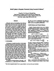
FEATURE-BASED MODELS The feature-based model of Sloman (1993) predicts inductive strength as a measure of feature overlap between premises and conclusion categories. Like the similarity-coverage model, the feature-based model applies to arguments in

which premises and conclusion have the form “all members of have property

”. Moreover, Sloman’s (1993) model mainly focuses on “blank” predicates about which people would have few prior beliefs.

The feature-based model is implemented as a connectionist network in which a set of input nodes serves to encode features values, and an output node

serves to encode the blank predicate . To illustrate the process by which the

model determines inductive strength, Sloman (1993) considers the following argument: Robins have property

——————————— (S)

Falcons have property


The temporal evolution of the connectionist network for the argument (S) is shown in Figure 1.1. Before the presentation of the argument, the node representing the blank predicate is initially not connected to any nodes that represent the features of the premise category (Figure 1.1-a). Then, to encode the premise, the input nodes that represent the features of ROBIN are connected

to the predicate node . In this way, the input nodes ‘activate’ the predicate node (Figure 1.1-b). Finally, argument’s conclusion is tested by evaluating the extent

to which the predicate node becomes activated by means of the features of the conclusion category (Figure 1.1-c).

Figure 1.1: Temporal evolution of the network implemented in the feature-based model for the argument (S)


In brief, the model’s predictions are completely determined by a set of features and by two rules: an encoding rule and an activation rule. The encoding rule posits how connections are established between featural and predicate nodes, whereas the activation rule defines the value of predicate node. In other terms, the encoding rule allows the connectionist network to learn associations between input nodes and output node. Then the activation rule serves to measure what value is assigned to the output node after presenting the features of the conclusion category. If this value is high, then the argument in question is judged strong; if it is low, then the argument is judged weak. As highlighted by Sloman (1993) himself, according to the feature-based model, “argument strength is, roughly, the proportion of features in the conclusion category that are also in the premise categories”. And “intuitively, an argument seems strong to the extent that premise category features ‘cover’ the features of the conclusion category, although the present notion of coverage is substantially different from that embodied by the similarity-coverage model” (p. 242). Perhaps the most important difference between the feature-based model and the similarity-coverage model is that the former does not have a specific component for assessing coverage of a superordinate category. In fact, the feature-based model is able to address many of the same phenomena as the similarity-coverage model, but without employing a second mechanism apt to coverage. Another difference between the two models is that only Osherson et al.’s (1990) model assumes that judgments of inductive strength depend on a stable hierarchical category structure. By contrast, the feature-based model assumes that inductive strength depends on the intensity of connection between the features of the conclusion category and the predicate in exam. Here, the existence of a stable category structure is not necessary. Obviously, Sloman (1993) recognizes that people have some knowledge about the hierarchical structure of categories. However, in his model, this knowledge is not represented as structured as would be required to support Osherson et al.’s (1990) model.


Both the similarity-coverage model and feature-based model make accurate predictions of the inductive strength of arguments whose predicates are blank. Yet, as noted by Heit (1998), inductive reasoning with blank properties captures only one aspect of inductive reasoning in general.

BAYESIAN MODELS Heit (1998) proposed a more extensive framework for addressing phenomena besides similarity, diversity, and typicality effects. He has presented a theory where induction is modeled as Bayesian inference. Hence, the name of his model: Bayesian model. To illustrate the model, Heit (1998) discusses the following inductive argument involving just two categories of animals, namely, cows and horses: Cows have property

—————————— (H) Horses have property

The author argues that, when reasoning about novel properties to be attributed to cows and/or horses, it is convenient to classify all the known properties concerning animals into four groups: 1. properties that are true of cows and horses; 2. properties that are true of cows but not horses; 3. properties that are true of horses but not cows; 4. properties that are not true of either cows or horses. These four types of known properties are thought of as four alternative hypotheses, each associated with a degree of prior belief. Table 1.3 reports the degree of prior belief that Heit proposes for each of the four hypotheses. The value of 0.70 assigned to hypothesis 1 indicates that there is a 70% chance that a new property would be true of both cows and horses. Heit (1998) observes that the prior beliefs sum up to 1, since the corresponding hypotheses are exhaustive and mutually exclusive.


Table 1.3: The four hypotheses and the degree of prior beliefs used in Heit’s (1998) example

Hypotheses 1 Cow = True and Horse = True 2 Cow = True and Horse = False 3 Cow = False and Horse = True 4 Cow = False and Horse = False

Degree of prior belief 0.70 0.05 0.05 0.20

Once the prior beliefs are assigned, the next step planned in the Bayesian model is to update the belief values in light of new evidence. As for argument (H) above, the prior beliefs concerning the four hypotheses need to be updated in light of

the premise “Cows have property ”. To compute the posterior degree of belief

in each hypothesis, Bayes’s theorem is used and the values obtained are 0.93 for hypothesis 1, 0.07 for hypothesis 2, and 0 for the remaining hypotheses 3 and 4.

At this point, Heit (1998) argues that the previous values may be used to assess the plausibility of the argument’s conclusion. Indeed, by virtue of the total

probability theorem, the degree of belief that horses have property is directly given by summing the updated beliefs in hypotheses 1 and 3, namely, the values 0.93 and 0.

Heit (1998) observes that, before learning that cows have the property ,

the prior belief that horses have the property is only 0.75 = 0.70 + 0.05. Thus,

according to the model, the premise that cows have the property leads to an increase in the belief that horses have the property . However, in Heit’s (1998)

Bayesian model the inductive strength of an argument is not measured as a function of the increase in the plausibility of its conclusion. Inductive strength is simply given by the updated plausibility of the argument’s conclusion. It is worth noticing that the Bayesian model is strictly linked to accounts of hypothesis testing and, as such, it suggests a normative description on how to reason with a hypothesis space. This account is rather successful as it is able to accommodate most of the psychological phenomena as Osherson et al.’s (1990) and Sloman’s (1993) models. On the Bayesian model account, assessing the


strength of an inductive argument is regarded as learning about the property appearing in the premises and conclusion of that argument. For example, upon

learning that dogs have some novel property , one might wonder whether

wolves or parrots have the same property . The key assumption of the Bayesian

model is that, to answer this question, people would analyze a set of hypotheses

about the novel property, relying on prior knowledge about familiar properties. For instance, the fact that people know a relatively large number of properties true of both dogs and wolves may lead to the conclusion that, if property is

applied to dogs, then it probably applies to wolves too. On the other hand, a relatively small number of properties are known to be true of both dogs and

parrots, and this may lead to conclude that property is relatively unlikely to extend to parrots.

The foregoing example is consistent with the principle that similarity promotes property projection. Given the premise that a category has a certain property, it seems plausible that a similar category has that property as well. But, for some properties and some categories, similarity does not seem to be central to inductive inferences. Heit and Rubinstein (1994) have provided the following important example showing how inferences may go in the opposite direction of what overall similarity would predict.

Chickens prefer to feed at night —————————————— (HR-1) Hawks prefer to feed at night

Tigers prefer to feed at night ————————————— (HR-2) Hawks prefer to feed at night

Heit and Rubinstein (1994) found that the argument (HR-1) is judged weaker than the argument (HR-2). But, if the behavioral property about feeding and predation is replaced with the blank, biological property “have a liver with two


chambers”, then the standard trend predicted by the similarity-coverage model re-emerges. Despite the considerable biological differences between tigers and hawks, it seems that people are influenced by the known predatory behavior that these two animals have in common. Another example in which similarity seems not to be central to induction has been provided by Smith, Shafir, & Osherson (1993).

Poodles can bite through barbed wire —————————————————————— (SSO-1) German Shepherds can bite through barbed wire

Dobermans can bite through barbed wire —————————————————————— (SSO-2) German Shepherds can bite through barbed wire

Smith et al. (1993) found that the argument (SSO-1) is stronger than the argument (SSO-2), even though there is greater similarity between Dobermans and German Shepherds than between poodles and German Shepherds. An informal justification given to this result is based on the preconditions for the capacity to bite through barbed wire: if a little and weak dog, like a poodle, is able to bite through barbed wire, then clearly a German Shepherd, which is stronger and more ferocious, can do so as well. Heit (1998) shows how his Bayesian model can account for effects (e.g., those presented in the previous two examples) that are determined by properties rather than by the similarity between categories. The distribution of prior beliefs across hypotheses is of extreme importance to predict these effects. But how are these prior beliefs generated? According to Heit, prior beliefs are assigned on the basis of past observations. His explanation for how prior beliefs come about is heavily memory-based: the probability of a hypothesis is proportional to the number of familiar features that can be retrieved from memory and that have the same extension as that hypothesis.


Tenenbaum et al. (2007) acknowledge that, if supplied with the right kinds of prior beliefs, Heit’s (1998) Bayesian model is able to predict a number of qualitative phenomena concerning both blank and non-blank properties. However, Tenenbaum et al. (2007) point out the lack of a formal method for generating priors, as well as the lack of any quantitative test for checking the accuracy of the model through people’s judgments.

THEORY-BASED BAYESIAN MODELS Tenenbaum, Griffiths, & Kemp (2006) have proposed a framework that adopts a Bayesian approach which is similar to that implemented by Heit (1998). The Bayesian approach of Tenenbaum et al. (2006) attempts to answer two important kinds of question about human inductive capacities. First, what knowledge is a given inductive inference based on? And second, how does that knowledge support property generalization? In contrast with previous models of inductive reasoning, in which the emphasis is put mainly on the process of induction, the approach developed by Tenenbaum et al. (2006) takes the prior knowledge representation as a crucial element. A major distinction between the Bayesian model of Heit (1998) and the theory-based Bayesian framework of Tenenbaum et al. (2006) is the presence, in the second framework, of a mechanism that generates appropriate prior beliefs. The framework proposed by Tenenbaum at al. has two main components: a structured probabilistic representation of domain-specific knowledge, and a general Bayesian inference engine to perform inductive inferences. Even though structured representations are far from being complete formalizations of people’s knowledge, they are important because they approximate the genuine structures contained in the world. On the other hand, Bayesian inference provides a well-grounded normative procedure for uncertain reasoning. Together, the two components lead to quantitative models for predicting people’s inductive judgments. More importantly, the two components offer an explanation about the processes underlying inductive reasoning.


It has been argued that different properties, such as anatomical features, behavioral properties, or disease states of animal species, might promote different patterns of inductive behavior. But whether this is due to diverse kinds of knowledge, diverse mechanisms of reasoning, or both, is not so clear. According to Tenenbaum et al. (2007), a single Bayesian mechanism, in which the priors are generated to capture most of the knowledge that supports induction, may be sufficient. It is challenging to adequately model prior beliefs concerning any familiar thing, because different kinds of knowledge might be relevant when making inferences about the thing in question. For example, a cat can be thought about in a large number of ways. It is an animal that belongs to the category of felines, eats mice, climbs trees, has whiskers, and so on. As pointed out by Tenenbaum et al. (2007), all of these pieces of information could be influential in an inductive inference about cats. For instance, upon learning that cats suffer from a recently discovered disease, people could suspect that mice have that disease too. Or, upon learning that cats have a recently discovered gene, people could think that tigers are more likely to have that gene than mice. Thus, as mentioned earlier, it seems clear that inductive inferences crucially depend on the property involved. The theory-based Bayesian models of Tenenbaum et al. (2006), as well as the Bayesian model of Heit (1998), accounts for property-based phenomena by positing that people can rely on different kinds of prior knowledge. For Tenenbaum et al. (2006) any computational theory on inductive reasoning should show as explicitly as possible how priors are generated in a specific context. As regards the theory-based Bayesian framework, two aspects are most relevant for constructing priors: firstly, a representation of how categories are related to each other and, secondly, a process that governs how properties are distributed over categories. In this framework, each category is represented as a node in a relational structure. The structure’s edges represent relations that are relevant for determining inductive strength (e.g., taxonomical or causal relations). Priors are then generated by means of a stochastic process defined over the relational structure. Stochastic processes, such as diffusion


process, drift process, or noisy-transmission process, can be used to model how properties are distributed over the related categories. The theory-based Bayesian framework of Tenenbaum et al. (2006) is able to capture several kinds of knowledge by choosing the appropriate kind of structure and the appropriate stochastic process. However, an important constraint in the construction of priors is given by the correspondence, albeit not perfect, between the structure of the world and the representation of the Bayesian model. To illustrate, the theory-based Bayesian model developed for generic biological properties uses a noisy-mutation process over a taxonomic tree. The theory-based Bayesian model developed for causally transmitted properties, instead, uses a noisy-transmission process over a predator-prey network. Both models are built by thinking about how some class of properties is actually distributed in the world. Not surprisingly, they correspond roughly to models employed by biologists and epidemiologists, respectively. According to Tenenbaum et al. (2006), by deriving prior beliefs from ‘intuitive theories’ (e.g., intuitive biology, intuitive physics, intuitive psychology) that reflect the actual structure of the world, it becomes clear why these priors should support induction in real-world tasks. It is worthwhile to note that the theory-based approach uses the same Bayesian principle to explain how intuitive theories guide inductive inferences, but also how intuitive theories might be learned from experience. Both the model for generic biological properties and the model for causally transmitted properties have been tested. In doing so, judgments of inductive strength expressed by participants have been compared with theoretical judgments predicted by the models. In addition, a comparison with several alternative models, including the similarity-coverage model, has been performed (see Tenenbaum et al., 2007). In general, the theory-based Bayesian model that is specific for the inductive context in exam has given better predictions than, or comparable to, the best of the other models. As pointed out by Sloman (2007), the sophisticated framework proposed by Tenenbaum et al. (2006) is impressive in its potential for generating domain-


specific models. The strength of this approach is that it offers a perspective covering induction in all its forms. However, the danger is that a large number of relational structures need to be created, each shaped to fit a specific study. Yet, it is plausible to think that relational structures are not independent of each other. Presumably, all rational structures are generated on the basis of some fundamental principles. For example, a top-down biological structure might emerge from a causal analysis grounded on an evolutionary base. In fact, it might be the case that, once the causal analysis that endorses the hierarchical structure is clearly defined, the structure itself will turn out to be unnecessary. In this sense, inductions might be mediated directly by causal knowledge. In other words, the relational structure may serve as a proxy for some other kind of knowledge, like causal knowledge, that is not domain specific. This last view was largely supported by Rehder (2007).

INDUCTIVE REASONING REVISITED AS CAUSAL REASONING Rehder (2007) interprets property generalization in terms of causal reasoning. He reports numerous sources of evidence that people reason causally when they generalize properties. For example, he mentions the results of Heit and Rubinstein (1994) showing that a behavioral property (e.g., “travel in a zig-zag path”) is projected more strongly from tunas to whales than from bears to whales. But when the property in exam is biological (e.g., “have a liver with two chambers”), then a reversal trend is observed, that is the property is generalized more strongly from bears to whales than from tunas to whales. Rehder’s reading of these results is that people recognize the biological similarity between bears and whales because of a causal mechanism associated with their common category, namely, MAMMAL. Probably this mechanism gives rise to biological properties like having a two-chambers liver. On the other hand, people think that tunas and whales are more likely to share a behavioral property like traveling in a zig-zag path, because tunas and whales are prey/predator animals living in the same natural environment.


Also the results of Smith et al. (1993), already illustrated above, are interpreted by Rehder in terms of causal reasoning. Smith et al. (1993) found that people are more willing to generalize the property “can bite through barbed wire” to German Shepherds from poodles than from Dobermans. In this case, the kind of causal reasoning that drives people’s judgment is more or less the following: if poodles can bite through barbed wire, then obviously stronger dogs like German Shepherds can do it too. But it could not be the case if the premise category is another powerful dog. Finally, another example used by Rehder in support of the centrality of causal reasoning in property generalization is due to Sloman. Sloman (1994) considers the following pair of arguments:

Many ex-cons are hired as bodyguards ——————————————————— (S-1) Many war veterans are hired as bodyguards

Many ex-cons are unemployed ———————————————— (S-2) Many war veterans are unemployed

According to Sloman’s (1994) results, the argument (S-1) is judged stronger than the argument (S-2). Rehder’s explanation is that, in the first argument, the same reasons that lead to be a good bodyguard (e.g., being experienced fighter) can be applied to both ex-cons and war veterans. By contrast, the reasons that explain unemployment of war veterans are less likely to be applied to ex-cons too. Rehder (2006) has developed a general theory that underlines the centrality of causal reasoning in induction. This theory makes three predictions about the role of causal reasoning in category-based generalizations. The first prediction is that property generalization can reflect prospective reasoning. According to this prediction, the more the causes producing a property are present in the conclusion category, the more the property is generalizable. The


second prediction is that property generalization can be driven by a diagnostic reasoning. The more the presence of a property can be inferred by the effects it might produce, the more the property is generalizable. To put it differently, property generalization can be thought of as a particular kind of causal reasoning in which people make a diagnosis about the presence of a property by analyzing whether its symptoms (i.e., effects) are present or not. The third prediction is that property generalizations are regulated by extensional reasoning. The more the causes and/or effects of a property are prevalent, the more the property is generalizable. The previously discussed results of Heit and Rubinstein (1994), Smith et al. (1993), and Sloman (1994) can be seen as empirical support for the prospective-reasoning prediction (for other empirical data in support of Rehder’s theory, see Rehder, 2006). An important question concerns how causal knowledge interacts with the phenomena formalized by the similarity-coverage model, such as diversity, similarity, and typicality. To foreshadow the main result, research suggests that causal reasoning not only influences property generalizations, but, in some cases, it may replace the similarity-based effects. For example, Lopez, Atran, Coley, Medin & Smith (1997) found that Itzaj Maya, a population in the rainforest of Guatemala with great expertise regarding local plants and animals, often based their inferences (e.g., about the disease in a species) on causal processes, thus failing to show standard diversity effects. By contrast, American undergraduates did show standard diversity effects on the same items. Of course, the foregoing results could be explained in terms of cultural differences between Itzaj and Americans. However, the prevalence of causal explanations does not seem to be attributable only to cultural factors. Proffitt, Coley, & Medin (2000) studied inferences about plant categories made by three groups of American tree experts: taxonomists, landscapers, and tree maintenance workers. The aim was to test whether and how property generalizations are influenced by typicality and diversity effects. Like Itzaj Maya, the landscapers and the tree maintenance workers did not show standard


diversity effects. Moreover, none of the groups of tree experts exhibited standard typicality effects. The studies of Lopez et al. (1997) and Proffitt et al. (2000) tested experts with domain-specific knowledge, but there is also evidence, coming from nonexpert people, that proves a similar pattern. Consider the following pair of arguments proposed by Medin, Coley, Storms & Hayes (2003):

Pigs are injected with antibiotics Chickens are injected with antibiotics ———————————————— (MCSH-1) Cobras are injected with antibiotics

Pigs are injected with antibiotics Whales are injected with antibiotics ———————————————— (MCSH-2) Cobras are injected with antibiotics

Medin et al. (2003) found that American undergraduates judged the argument (MCSH-1) weaker than the argument (MCSH-2), despite the set of premise categories is more diverse in the first argument than in the second one. Maybe, pigs and chickens were recognized as farm animals, and this suggested possible causes of being injected with antibiotics. The fact that those causes are absent in cobras may have led to a weaker property generalization. To deepen the study on how causal knowledge interacts with typicality, diversity, and similarity effects, Rehder (2006) conducted three experiments in which the causal knowledge was explicitly provided to participants (observe that in the studies of Lopez et al., 1997; Proffitt et al., 2000; and Medin et al., 2003 participants’ judgments relied on background knowledge). In each experiment two factors were manipulated. One factor was the presence/absence of a causal explanation; the other factor was either diversity, similarity, or typicality. The results suggest that, if a causal explanation is available, then


typicality, similarity, and diversity effects can be reduced or completely eliminated.

AVAILABILITY AS A KEY FACTOR TO EXPLAIN CATEGORY-BASED INDUCTION The concept of availability is central for Shafto, Coley, and Vitkin (2007). These authors, too, recognize that many kinds of knowledge can support inductive reasoning, and that a specific knowledge would be employed in a given particular situation. For example, taxonomic knowledge would be preferred when reasoning about a novel property concerning internal features such as two-chambered liver; ecological knowledge would be preferred, instead, when reasoning about toxins or diseases that might spread through an ecosystem. But what are the factors that influence the selection of a particular knowledge in a given situation? Shafto et al. (2007) argue that different kinds of knowledge are differentially available across contexts, and that the ease with which specific knowledge comes to mind reflects the probability that such knowledge will guide inductive inference. According to Shafto et al.’s (2007) view, availability is a dynamic concept: it may change. The main sources determining changes in the availability of different kinds of knowledge are short-term influences of context and long-term effects of experience. On one hand, the context characterizing category-based induction tasks (e.g., the set of categories and the property used) results in acute changes in availability. On the other hand, prior knowledge accrued through experience results in chronic changes in availability. Shafto et al. (2007) reconsider evidence coming from experimental results in psychological literature, and they reinterpret existing phenomena in light of changes in availability. As will be seen, these changes are due to both inductive context and experience in a specific domain. As regards inductive context, the results obtained by Heit and Rubinstein (1994), which highlight the importance of property in induction, are explained as follows: the given property to be generalized makes the specific knowledge that drives inductive inference more available. Thus, in general, anatomical knowledge is more available when


anatomical properties are given, and likewise behavioral knowledge is more available if behavioral properties are provided. Another line of evidence, showing how context may change availability, concerns the effects of relations among premise categories, or among premise and conclusion categories. Work by Medin, Coley, Storms & Hayes (2003) has identified a number of effects, termed relevance effects, that demonstrate how salient relations among premises categories, or between premises and conclusion categories, may direct the assessment of inductive strength. One of these effects is non-diversity via property reinforcement. To illustrate, consider the following pair of arguments: Polar bears have property Antelopes have property

————————————— (MCSH-1)

All animals have property

Polar bears have property Penguins have property

————————————— (MCSH-2)

All animals have property

Medin et al. (2003) found that arguments like (MCSH-1) are rated stronger than arguments like (MCSH-2), even though, on a taxonomic account, the premises in the second argument offer better coverage of the conclusion category than the premises in the first argument. It seems that the salient property shared by polar bears and penguins – adaptation to a freezing environment – interferes with the greater coverage they provide to ANIMAL category. A second effect analyzed by Medin et al. (2003) is non-monotonicity via property reinforcement. Consider the following two arguments:


Brown bears have property

————————————— (MCSH-3)

Buffalo have property

Brown bears have property Polar bears have property

Black bears have property

Grizzly bears have property

————————————— (MCSH-4)

Buffalo have property

By virtue of the monotonicity phenomenon (see Osherson et al., 1990), the argument (MCSH-4) should be stronger than the argument (MCSH-3). However, Medin et al. (2003) found an opposite trend. A possible explanation is that the

premises in the argument (MCSH-4) seem to reinforce the idea that property is involved with bears, and therefore the property is unlikely to be true of buffalo.

Shafto et al. (2007) reinterpret the relevance effects reported by Medin et al. (2003) as follows: if specific relations among premises and/or conclusions categories are available (e.g., being polar animals or bears), then more general phenomena are overcome (e.g., diversity or monotonicity effects). The results examined so far are all explained in terms of acute changes in availability due to factors that outline inductive context: the nature of property and the relations between categories in an argument. Shafto et al. (2007) also present evidence that the availability of different kinds of knowledge can be mediated by experience in a specific domain. For example, evidence in this direction comes from the results of Lopez et al. (1997), and Proffitt et al. (2000), which reveal that novices and experts rely on different kinds of knowledge when making inductive inferences. It is worth noticing that Rehder (2007) used the same results – Lopez et al. (1997) and Proffitt et al.’s (2000) results – to prove how causal reasoning may guide induction. By contrast, Shafto et al. (2007) use


those results to show that experiential background may lead to chronic changes in the kinds of knowledge that are available for inductive reasoning. In sum, Shafto et al. (2007) maintain that the notion of availability provides a framework which is able to connect a large number of phenomena related to category-based induction. This framework can explain the effects of properties on inductive reasoning, and can also account for the influence of experience in property generalizations.

45

Chapter 2 In case of uncertain evidence

2.1 The role of uncertainty in everyday life: a psychological perspective

Uncertainty in everyday life is often understood as a part of some underlying, causal structure of the world that people strive to comprehend. According to Hastie and Dawes (2001), people tend to deny the existence of chance. Or, even worse, people tend to conceive some rationale to explain life’s uncertainties. Sometimes, the consequences of denying uncertainty and believing in a deterministic world can be very severe. Some individuals think that poor people, living on the street, must have done something to deserve that fate. And these poor people themselves may accept that judgment. In such a situation, assistance measures are rendered ineffective. Even those who have studied the theory of probability calculus are inclined to erroneously interpret the behavior of random processes unless they are asked to corroborate their interpretations. A typical misconception about randomness is to believe that some kinds of chance events, such as winning the lottery, involve skills. This misconception is caused by the fact that, in such events, there is an element of active participation. For instance, we have to choose a lottery ticket, if we want a chance of winning. Choosing the right ticket is often seen as a special ability. But, of course, this reading is not correct. It may lead to an illusion of personal control over situations that are governed solely by chance. According to Hastie and Dawes (2001), it is very easy to confuse factors depending on chance with factors based on skill. When evaluating the outcomes

46 2. In case of uncertain evidence

of actions that involve both chance and skill (e.g., making a goal in a football match), people have a strong propensity to repeat behaviors that precede success and change behaviors that precede failure. Such a strategy encourages superstitious behaviors. Superstitions, as well as beliefs in tarot cards and astrology, help many people to make sense of uncertainty in life. It is not pathological to try to reduce uncertainty regarding our existence and the environment around us. Uncertainty reduction is essential to the cognitive enterprise of understanding the world. It is fundamental even in science. However, a complete removal of uncertainty would be dreadful. In Prometheus Bound, Aeschylus writes:

Prometheus: I caused mortals to cease foreseeing their doom. Chorus: Of what sort was the cure that you found for this affliction? Prometheus: I caused blind hopes to dwell within their breasts. Chorus: A great benefit was this you gave to mortals. (Aeschylus, Prometheus Bound, vv.250-253, Smyth, 1926)

According to Aeschylus, hope comes from the lack of certainty of doom. Hope is blind. A life without uncertainty would be unbearable: no hope, no challenge, no freedom. Imagine the horror of being informed to have a gene that causes Alzheimer’s disease with certainty. But being informed about pleasant news with certainty would also detract from life’s happiness. It is only because people do not know what the future holds for them that they can have hope. It is only because people are unaware of the exact consequences of their choices that choice can be free, within the limits of morality.

47 The role of uncertainty in everyday life: a psychological perspective

Most people recognize that there is a lot of uncertainty in the world. A very critical choice is whether to accept that uncertainty or try to avoid it. Those who choose to reject uncertainty, or those who believe uncertainty does not exist, live in a stable, deterministic world, which is constructed, invented, not real. By contrast, those who accept uncertainty can appreciate the limits of knowledge. A central part of wisdom is the capacity to establish what is uncertain, and comprehend the probabilistic essence of uncertainty in real contexts. Both in the epistemological and psychological domain, uncertainty is normally expressed and formalized in terms of probabilities. It is usual to assign a different degree of uncertainty, i.e., a different probabilistic value, to alternative hypotheses under examination. Yet, in epistemological and psychological research, much less attention has been paid to another kind of uncertainty, which is likewise central: the uncertainty relative to a piece of evidence. In

the

following

section,

I

will

show

how

classical

Bayesian

conditionalitazion can be extended in order to account for situations where a piece of evidence is not certain.

2.2 On Jeffrey’s rule Jeffrey conditionalization represents a formal means to update degrees of belief on the basis of uncertain evidence. In what follows, I will illustrate Jeffrey’s rule in some details. Consider a non-empty set of propositions Γ closed under negation,

conjunction and disjunction, and consider a probability function Z defined, at a

given time [, over Γ. Suppose that O is a set of mutually exclusive and jointly exhaustive events, with O Γ and Z O 0 0 for all \. Jeffrey (1965) has given the following definition to introduce his conditionalization:


Definition 2.1: A probability measure ] is said to come from Z , by

probability kinematics on O , if there exists a sequence Ô of positive real numbers summing to one, such that

] ! ∑O Z |O = Ô , for all Γ.

(2.1)

Observe that, if the set O is comprised by only one proposition , then the

formula (2.1) reduces to the following:

] ! Z | , for all Γ.

(2.2)

Thus, probability kinematics turns out to be a generalization of classical Bayesian conditionalization. As Wagner (2002) points out, the formula (2.1) is equivalent to the conjunction of two conditions: ] O ! Ô ,

for all \, and

(2.3)

] |O ! Z |O , for all Γ and for all \.

(2.4)

Put into words, probability kinematics provides a tool to revise a probability function when the total evidence induces a revision of the probabilities of O – as

specified by (2.3) – and when nothing new is learned about the relevance of any O to every proposition – as specified by (2.4). It is worth noting that the

probabilities ] O are based not only on new evidence, but also on old evidence.

Although Jeffrey conditionalization appears in many respects to be the most appropriate generalization of Bayesian conditionalization, many authors have objected that Jeffrey conditionalization is defective, for it is noncommutative.

This

means

that

consecutive

applications

of

Jeffrey

conditionalization may produce different ultimate results, depending upon the

49 On Jeffrey’s rule

order in which those conditionalizations are applied. For example, having

revised Z to ] by the formula (2.1), consider a subsequent revision of ] to ` by an analogous formula:

` ! ∑b ] R|ab W = cb , for all Γ,

(2.5)

where dab e and Rcb W have the same functions as the previous O and Ô . Now

imagine reversing the order of the revisions, so that Z is first revised to ]f by means of dab e and Rcb W, and then ]f is revised to `f by means of O and Ô . It may be the case that ` g `f, unless O = and dab e = a. Under classical

Bayesian conditionalization, in fact, ` ! Z |

`f .

a ! Z |a

!

In what follows, I will discuss a numerical example, due to Lange (2000),

showing the non-commutativity of Jeffrey’s rule. Imagine seeing a bird at twilight, and imagine identifying it to be a raven. Consider the following propositions: ! “All ravens are black”,

! a ! “The bird observed is black”. Because of the darkness, it is difficult to identify the bird’s color with certainty. So suppose that the observation made at twilight can only raise the confidence in

from Z ! 0.75 to ] ! 0.99. Suppose, moreover, that initially

Z

Jeffrey

! 0.7 and Z conditionalization,

! 0, so that Z ! 0.7. According to

] ! @l.mnE = 0.99 M @l.nE = 0.01 ! 0.924.

particular, it results that ]

l.m

l

! 0.924 and ]

In

! 0. Now,

suppose that a second glance lowers the confidence in , so that ` ! 0.8. A

second application of Jeffrey’s rule yields ` r 0.747.

If, instead, the two experiences occur in a reversed order, namely,

]f ! 0.8 and `f ! 0.99, then ]f r 0.747 and `f ! 0.924. The


main steps in the two cases are summarized in the following sequences of revisions. Z ! 0.7 Z ! 0.75

> > > ] ! 0.99

Z ! 0.7 Z ! 0.75

> > > ]f ! 0.8

] ! 0.924

]f r 0.747

> > > ` ! 0.8

` r 0.747

> > > `f ! 0.99

`f ! 0.924

(2.6)

(2.7)

In both sequences, the second glance completely overrides the first glance. Thus, apparently, commutativity is not respected: ` g `f .

The possibility of such non-commutativity has caused much concern

among several epistemologists. Van Fraassen (1989) writes about this issue:

Two persons, who have the same relevant experiences on the same day, but in a different order, will not agree in the evening even if they had exactly the same opinions in the morning. Does this not make nonsense of the idea of learning from experience? (van Fraassen, 1989, p. 338)

Following Lange (2000), I will argue that Jeffrey conditionalization has been deemed inadequate on the basis of unjustified concern. Returning to the foregoing example, the fact that two persons assign probability values to in a reversed order does not mean that those persons have identical learning from the same relevant experiences. Observe that the last step in the sequence (2.6) and the first step in the sequence (2.7) are both induced by experiences

prompting a revision of the belief in , with the effect of setting ! 0.8. Yet,

these experiences are not the same. The main reason is that the degree of

51 On Jeffrey’s rule

confidence in , directly prompted by an experience, depends on agent’s prior opinions. In order to explain this, Lange writes:

For an experience at twilight to have lowered our confidence in E from 0.99 to 0.8, the bird must have not looked much the way a black bird would be expected to look at twilight, whereas for an experience at twilight to have raised our confidence in E from 0.75 to 0.8, the bird must have looked about the way that any dusky colored object would be expected to look under those conditions. Plainly, these are different experiences. (Lange, 2000, p. 398)

Though Jeffrey’s rule may give different ultimate outcomes depending on the order in which probability values are plugged in, this does not prove its noncommutativity. Indeed, the raven example does not show that Jeffrey conditionalization leads to different final opinions, starting from the same priors and the same experiences. According to Wagner (2002), the concern about the non-commutativity of Jeffrey’s rule seems to rely on implicit acceptance of the following two principles: Principle 1: If the experience inducing the revision of Z to ] and the

experience inducing the revision of ]f to `f produce the same learning,

and if the experiences inducing the revision of ] to ` and the

experience inducing the revision of Z to ]f produce the same learning,

then it ought to be the case that ` ! `f .


Principle 2: Identical learning deriving from the revision of Z to ]

and of ]f to `f ought to be expressed by the probability identities `f O ! ] O , for all \,

(2.8)

and identical learning deriving from the revision of ] to ` and of Z

to ]f ought to be expressed by the identities ]f Rab W ! ` Rab W, for all s.

(2.9)

While Principle 1 is wholly correct, Principle 2 is erroneous, since probabilities assigned to O and ab are based on the total evidence, as already mentioned

earlier. This is to say, probabilities appearing in the condition (2.3), which defines Jeffrey conditionalization, depend not only upon new evidence, but also upon old evidence, and thus they incorporate elements of the relevant priors. Within the Bayesian framework, it is possible to represent numerically what is learned from new evidence alone. The correct representation is provided by the ratios of new-to-old odds (see Good, 1950, 1983). Wagner (2002) proved that, if Principle 2 is modified by substituting (2.8) and (2.9) with adequate identities involving Bayes factors, then Principle 2 is both sufficient and, in many cases, necessary for the satisfaction of Principle 1. Put another way, once identical learning is appropriately formalized, Jeffrey’s rule does commute across order. The theoretical study presented in the following section4 addresses the issue of generalizing Bayesian theory of confirmation to cases of evidential uncertainty. As will be shown, Jeffrey conditionalization will play an essential role.

4

Much of the material in §2.3 appears in Crupi, Festa, & Mastropasqua (2008).

53

2.3 A theoretical study on how to adapt confirmation measures in case of evidential uncertainty

2.3.1 Introduction Bayesian epistemology postulates a probabilistic analysis of many sorts of ordinary and scientific reasoning. Also, contemporary Bayesians typically endorse a subjective reading of probability, i.e., interpret probabilities as degrees of subjective belief. Huber (2005) has provided a novel criticism of Bayesianism, whose core argument involves a challenging issue: confirmation by uncertain evidence, i.e., evidence which has not been ascertained. In order to assess Huber’s argument, it is crucial to combine Bayesian confirmation theory with Jeffrey conditionalization. In the present theoretical study, I will argue that, when properly merged with Jeffrey conditionalization, Bayesian confirmation theory escapes Huber’s criticism and yields some new and appealing results. The discussion will proceed as follows. First, I will outline a generalized version of Bayesian confirmation theory which can be readily applied under Jeffrey conditionalization. Then, I will review a crucial requirement at the core of Huber’s argument and show that it is equivocal. I will argue that on one reading it amounts to a compelling principle, whereas on an alternative reading it turns out to be highly implausible. Finally, I will show that the proposed account of Bayesian confirmation by uncertain evidence appropriately captures the former version of the requirement and violates the latter.

2.3.2 Uncertain evidence and Bayesian confirmation For the purposes of the present study, I will consider a non-empty set of statements Γ closed under truth-functional operators such as negation,

conjunction and disjunction. Bayesians commonly assume that, at a given time [,


the belief state of an agent concerning the statements in Γ is represented by a

probability function Z defined over that set.

It may occur that, from time [ to u, experiences a change in opinion

concerning a particular Γ (provided that Z is not extreme, i.e.,

0 5 Z 5 1). Therefore, one important question is: how should ’s beliefs in other statements belonging to Γ change as a consequence?

Up to the mid-1960s, Bayesians had a ready answer only for the special

case in which, at time u, has come to believe that is certainly true, so that

] ! 1 (and, correspondingly, ] ! 0). ‘Classical’ Bayesian updating

or conditionalization (BC) postulates that:

If ] ! 1, then for any Γ, ] ! Z |

(BC)

However, it may surely also occur that ’s degree of belief in changes from time [ to u without reaching certainty. What will be the value of ] then?

Richard Jeffrey has suggested a natural and elegant way to generalize classical Bayesian conditionalization (Jeffrey, 1965, Chapter 11; also see Jeffrey, 2004, pp. 53-55). In Jeffrey conditionalization (JC), it is assumed that: For any Γ, ] ! Z | = ] M Z | = ]

(JC)

Thus, in (JC) ] is computed as an average of the ‘old’ conditional probabilities of on vs. , weighted by the current probabilities of and

, respectively. Notice that (JC) is obtained directly by the formula (2.1)

supposing O ! , (see §2.2). It is easy to see that Jeffrey

conditionalization is a proper generalization of classical Bayesian updating in the sense that (JC) implies (BC) (not the converse). Under Jeffrey conditionalization, however, a change in belief about prompts the updating of the prior

probability Z to a new value ] which is generally not identical to

either the conditional Z | (except when does become certainly true) or

55 A theoretical study on how to adapt confirmation measures in case of evidential uncertainty

the conditional Z | (except when becomes certainly false), but rather

lies between those two values.

Now consider the Bayesian notion of confirmation. Bayesian confirmation theory has been commonly elaborated and applied on the background of classical Bayesian updating. The issue has been to formalize the impact on a

hypothesis on the (often implicit, and quite restrictive) assumption of evidence having been ascertained, i.e., precisely in case Z g ] ! 1.

Then is said to be confirmed iff ] ! Z | 0 Z and to be

disconfirmed iff ] ! Z | 5 Z . (If ] ! Z | ! Z ,

it is said that coming to know that is neutral for .)

Can Bayesian confirmation theory be extended to cases such that from

time [ to u the probability of changes, but the assumption of having been

ascertained at u is relaxed? In other terms, is there any natural way to parallel

Jeffrey’s generalization of classical Bayesian updating in the framework of confirmation, and provide a plausible probabilistic account of confirmation by uncertain evidence? In what follows, I will claim that the answer is in the positive. (In essence, I will be following a proposal already made in Festa, 1999, pp. 56-59.) It is well known that various alternative measures of confirmation have been proposed and defended by Bayesian theorists (see Festa, 1999; Fitelson, 1999; see also §1.1.2). For the purposes of the present study, it will be convenient to focus on a core set of such confirmation measures which share the following interesting property: they can be defined by means of a function c

depending only on | and , c being a strictly increasing function of

the former value and a non-increasing function of the latter. We will call such confirmation measures classically P-incremental. Classically P-incremental measures include: • the ‘difference’ measure, first defined by Carnap (1950/1962a, p. 361) as: H , ! | >


• the ‘ratio’ measure, first defined by Keynes (1921, pp. 150-155) as: J, !

|

• the ‘odds ratio’ measure, first conceived by Alan Turing (as reported by Good, 1950, pp. 62-63) as5: vJ, !

|⁄| ⁄

• and the following measure, recently discussed by Crupi et al. (2007)

L, !

)| > if | x ' 1 > (| > ' &

otherwise

9

Notice that, in the notation adopted here, ! Z whereas, under classical Bayesian conditionalization, | ! ] . Thus, when classical

Bayesian conditionalization applies, the above definitions can immediately be converted into: HZ,] ! ] > Z JZ,] ! vJZ,] !

5

] Z

] ⁄] Z ⁄Z

Advocates of measure vJ include Good himself (1950, 1983) as well as Fitelson (2001a).


LZ,] !

)] > Z ' 1 > Z

(] > Z ' Z &

if ] x Z otherwise

9

Here, the double subscript ‘[, u’ highlights the fact that confirmation is relative in

an important sense: it is crucial for confirmation (disconfirmation) of a hypothesis by a change in opinion about to occur in the shift from one

probability distribution, Z , to another, ] , such that Z g ] .

But now my claim is that these latter formulas already represent

straightforward ways to generalize the corresponding confirmation measures as usually defined in the literature. This is because HZ,] , JZ,] , vJZ,] and

LZ,] all measure (although in different ways) the departure from the initial

probability of – Z – of an appropriately updated probability ] . Under Jeffrey conditionalization, generalized confirmation will amount to the departure from prior probability not of the conditional Z | (which, again, is not attained except in the special case of having in fact being ascertained), but rather of the updated probability ] to which a change in belief about

the uncertainty of will lead. Clearly, for any classically P-incremental Bayesian

confirmation measure, a generalized version can be devised along these lines. Importantly, by such a move, any classically P-incremental measure will also

satisfy a generalized condition of P-incrementality, i.e., it will be expressible by

means of a function c depending only on ] and Z , c being a strictly increasing function of the former value and a non-increasing function of the latter.6

6

Such a generalized P-incrementality condition will play an important role in what follows. For

this reason, I am leaving aside here various confirmation measures proposed by Bayesian theorists which are demonstrably not P-incremental (see Carnap, 1950/1962a, p. 360; Nozick, 1981, p. 252; Mortimer, 1988, Section 11.1; Christensen, 1999, p. 449; Joyce, 1999, Chapter 6).


As a final remark, notice that, even beyond Jeffrey conditionalization, generalized P-incremental measures are suitable to application under any kind of updating rule considered in probability kinematics. This is because they only require defined values of Z and ] themselves, however related.7

2.3.3 Bayesian confirmation by uncertain evidence: test cases and basic principles

Huber (2005) has provided a useful hypothetical test case for Bayesian confirmation by uncertain evidence. Suppose: ! “All Scots wear kilts”,

! “The Scottish guy Stephen wears a kilt”.

Notice that (not the converse), so that the probability of the latter given the former must equal 1.8 Also, a Bayesian account would provide an agent

with initial probabilities Z and Z such that Z 0 Z , again

because of the logical relationship between the two statements. It is then assumed that is initially uncertain about both and , so that both Z and

Z are not extreme. It follows that coming to believe with certainty that “the

Scottish guy Stephen wears a kilt” would confirm “all Scots wear kilts”, i.e., Z | 0 Z .

7

Over the years, Bayesian theorists dealing with probability kinematics have considered various

forms of updating, as prompted by different kinds of information (see, for instance, van Fraassen, 1980; Jeffrey, 1992, Chapters 6–7). 8

Strictly speaking, in order to have , “Stephen is Scottish” should be included as a separate

background knowledge statement within Γ, and the notation should be modified accordingly. I embedded the statement “Stephen is Scottish” in simply for ease of exposition. This, however, has no effect on the issue discussed in the present study.


Suppose that , who is not wearing her glasses, looks at Stephen and

comes to subjectively believe that “the Scottish guy Stephen wears a kilt” with a moderate level of confidence, assumed to be represented by: ] ! 0.6. Importantly, Huber’s (2005) discussion of the example clearly suggests that ] 0 Z , i.e., that ’s observation has increased her confidence in .

Now consider looking at Stephen with her glasses on and coming to

subjectively believe that “the Scottish guy Stephen wears a kilt” with a high level of confidence, e.g., such that: ` ! 0.9.

Commenting on his example, Huber remarks that “if some E speaks in favor of some H – say, because it is a logical consequence of the latter – then [...] getting to know that E is probably true should provide confirmation for H – and the more probable it is that E is true, the more it should do so” (p. 105). Here I will focus on the last part of this statement, conveying the following comparative principle of confirmation by uncertain evidence: If coming to believe with certainty that would confirm , then,

the more probable it becomes that is true, the more this should confirm .

(H)

Huber considers various Bayesian confirmation measures, provides his own formal analysis of Bayesian confirmation in the ‘kilt’ case and argues that the difference measure H, the ratio measure J and the odds ratio measure vJ all violate the allegedly compelling principle (H). He concludes that serious doubts arise on the adequacy of the Bayesian approach and elaborates the point in various ways.


As Huber himself points out, however, his own example can be read in

two ways: (i) on one hand, ] and ` could be seen as referring to two alternative possible worlds, both branching from the state represented by Z ;

(ii) on the other hand, Z , ] and ` could be seen as following each other in a single time sequence. Importantly, Jeffrey conditionalization can be indifferently applied if either (i) or (ii) is adopted and, in both cases, it provides one unique

value for ] as well as one unique value for ` .9 Yet the distinction

between the possible worlds and the time sequence interpretation emphasizes that principle (H) is equivocal, as it can be taken as reflecting each one of two very different adequacy requirements imposed on a candidate measure of confirmation by uncertain evidence .

If the kilt example is read in terms of possible worlds, then the most

natural rendition of (H) is: Provided that Z | 0 Z , if Z 5 ] 5 ` , then Z,] 5 Z,` .

(H.1)

In words, this means that the higher the increase from the initial probability of an confirming the higher the confirmatory impact on will be.

If, however, the kilt example is read in terms of a single time sequence

(which is Huber’s main line in his paper), then principle (H) can also be seen as stating:

9

One may doubt that ` will remain equal when arrived at from Z vs. from ] , i.e., that Z | = ` M Z | = ` ! ] | = ` M ] | = ` .

This will be so, however, by virtue of a condition known as rigidity (Jeffrey, 1965, Chapter 11) or invariance (Jeffrey, 2004, p. 52), according to which Z | ! ] | and Z | !

] |. It can be proven that rigidity is implied by Jeffrey conditionalization (indeed, it is

logically equivalent to it).


Provided that Z | 0 Z , if Z 5 ] 5 ` , then Z,] 5 ],` .

(H.2)

As compared to (H.1), this is a completely different claim: it means that any

subsequent increase (no matter how small) in the probability of an confirming

will have a greater confirmatory impact on than any previous increase (no

matter how large) in the probability of .

My claim here is that, while (H.1) is a perfectly safe and sound intuitive

constraint on an adequate theory of confirmation by uncertain evidence, (H.2) is utterly implausible (as it will be argued shortly).

As for (H.1), it can be shown that (see the Appendix ~ for a proof):

Theorem 2.1: Any Bayesian confirmation measure Z,] enjoying generalized P-incrementality satisfies (H.1).

By contrast, in appropriate cases all alternative confirmation measures considered here will agree in violating (H.2) – as they should. In fact, it is easy to

conceive examples where the increase from ] to ` is so much smaller

(on any plausible standard of comparison) than the increase from Z to ] that (H.2) is a highly unappealing principle. To illustrate, suppose that:

Z | ! 1,

Z ! 0.05, Z ! 0.10,

] ! 0.80, ` ! 0.81.


By Jeffrey conditionalization, it can be computed that: ] ! 0.40,

` ! 0.405. Then: HZ,] ! ] > Z ! 0.35 0 0.005 ! ` > ] ! H],` . Similarly, it can be computed that: JZ,] ! 8 0 1.0125 ! J],` ,

vJZ,] r 12.667 0 1.021 r vJ],` , LZ,] r 0.368 0 0.008 r L],` .

Thus, all four confirmation measures considered here appropriately violate (H.2) in simple clear-cut cases, i.e., when a subsequent increase in the probability of an confirming is unequivocally very small (e.g., 0.80 to 0.81) as compared to a previous increase in the probability of the same (e.g., 0.10 to 0.80).10

10

It is fair to say that this line of argument is partly anticipated, and criticized, by Huber (2005)

towards the end of his paper (pp. 111ff.). Huber’s critical point essentially amounts to the

remark that, when uncertain evidence is at issue, Z,] crucially depends on Z even in qualitative terms (confirmation vs. disconfirmation). This seems, however, an appropriate

feature of Bayesian confirmation by uncertain evidence. Indeed, should it be the case that – for any reason – looking at Stephen actually decreased ’s confidence in down to 0.6 from an

initially higher value, we would like to say that this has disconfirmed to some extent. In fact, in

such a situation, Z,] would assume a negative value, since by Jeffrey conditionalization ] would itself be lower than Z . (Also see footnote 11.)


In conclusion, contrary to Huber’s claim, Bayesian confirmation theory, when properly generalized, actually gets things right when it comes to confirmation by uncertain evidence – i.e., satisfies principle (H.1) and violates (H.2).11

11

The lack of an explicit unpacking of statement (H) may not be the only reason why Huber

(2005) thinks otherwise. From his analysis, it seems that a further reason boils down to his own way of applying Bayesian confirmation under Jeffrey conditionalization. To illustrate, consider the ‘difference’ measure of confirmation. In line with the notation utilized so far, Huber (2005, p. 104) seems to have primarily employed the following way of computing degrees of confirmation: HZ,] ! ] | > ] .

This is unfortunate, however, for this quantity does not measure the departure of the

appropriately updated probability of from the initial one. In fact, under Jeffrey

conditionalization, it seems obvious that ] , and not ] |, represents the degree of

belief in at time u – when the probability of has shifted to non-extreme values – whereas

is adopted, Z , and not ] , represents the initial degree of belief in . Indeed, if HZ,]

not only the implausible principle (H.2), but even the compelling requirement (H.1) itself will be systematically violated. This is bad enough, but it gets worse. For HZ,] implies that even a

decrease in the probability of a confirming will confirm . In fact, it can be proven that, for

whatever (non-extreme) value of Z and ] , provided that Z | 0 Z , HZ,]

will be higher than the neutrality value 0. In the presence of what I see as a highly plausible alternative way to apply Bayesian confirmation to uncertain evidence, which does not exhibit

such undesirable properties, the latter remarks seem to show the inadequacy of HZ,] – not of

Bayesian confirmation theory itself.

64

65

Chapter 3 An experimental study on inductive reasoning with uncertain evidence

3.1 Aim of the study Judgments concerning the support that a piece of information brings to a hypothesis are commonly required in scientific research as well as in other domains (medicine, law). A major aim of a theory of inductive reasoning is to provide a proper foundation for such confirmation judgments. Previous research has shown that, after acquiring some pieces of certain evidence, intuitive assessments of inductive confirmation can be elicited directly, as people prove able to appropriately distinguish between posteriors and degrees of confirmation (see Tentori, Crupi, Bonini, & Osherson, 2007). It has also been observed that intuitive confirmation judgments based on ascertained

evidence tend to conform to normatively appealing models such as K and L (see

Crupi, Tentori, & Gonzalez, 2007).

However, in a large number of real situations, the evidence available is not certain, and the psychology of confirmation by uncertain evidence appears to have remained unexplored so far. The present experimental study aims at answering the following basic questions: • Do judgments of inductive strength depend on the degree of evidential uncertainty? • To what extent of accuracy can people judge the impact of an uncertain piece of evidence on a given hypothesis?

66 3. An experimental study on inductive reasoning with uncertain evidence

Two experiments have been carried out in an attempt to investigate whether the noteworthy results of previous studies on confirmation can be extended to scenarios involving uncertain evidence12.

3.2 Experiment I

3.2.1 Introduction Uncertainty is recognized as a ubiquitous challenge for human cognition and theories thereof (see, e.g., Hastie & Dawes, 2001; Jeffrey, 1992; Oaksford & Chater, 2007). Nonetheless, major theoretical accounts of reasoning typically assume some evidence to be known with certainty and to play a crucial role. Bayesianism is no exception, at least in its ‘textbook’ versions (Hartmann, 2008): a Bayesian agent is supposed to evaluate hypotheses by probabilistically conditionalizing on data that are acquired as certain. As useful as it may be for epistemological analysis, the latter assumption amounts to a rather crude simplification in psychological terms, as it is rarely met in real settings. In a murder trial, for instance, the defendant’s presence at the scene of the crime may be highly relevant for the hypothesis of guilt, yet it can hardly be completely ascertained in a court of law. At best, a DNA test or a reliable testimony can make it very probable. Indeed, in a variety of situations, people may need to assess the impact of a piece of evidence with probabilities that significantly change without attaining extreme values. Psychological research on inductive reasoning has largely shared the focus on ascertained evidence. For instance, from seminal inquiries up to more recent developments, the categorical induction paradigm presents participants with the consideration of a hypothesis/conclusion (e.g., “Birds have an ulnar 12

Much of the material in §3.2, §3.3, and §3.4 appears in Mastropasqua, Crupi, & Tentori

(submitted).

67 Experiment I

artery”) as possibly supported by an allegedly known fact given as a premise (e.g., “Robins have an ulnar artery”) (see, e.g., Osherson et al., 1990; Heit, 1998; Medin et al., 2003; Blok, Medin, & Osherson, 2007; Blok, Osherson, & Medin, 2007; Kemp & Tenenbaum, 2009). Now that a considerable amount of data and theorizing has been accumulated, it seems of interest to extend the empirical study of inductive reasoning beyond the limits of this framework, addressing how uncertain evidence is employed in hypothesis evaluation. In what follows, two experiments concerning assessments of the inductive impact of uncertain evidence will be presented. Before that, however, I will need to briefly illustrate the relevant theoretical framework which extends the basic Bayesian account to the uncertain evidence case. The two experiments will then provide an empirical test of the descriptive adequacy of this normative benchmark.

JEFFREY’S RULE OF CONDITIONALIZATION

Consider a pair of complementary hypotheses of interest and (extending

the following treatment to any richer partition is straightforward). In the

Bayesian framework, it is assumed that, at a given time N, the belief state of an agent is represented by a probability function defined over and . It may occur that, from time N to N M 1, the agent experiences a change in opinion

concerning a further statement – provided that is not extreme to begin

with, i.e., 0 5 5 1. Jeffrey conditionalization provides a natural way to

update the probability values of and , in case the agent’s degree of belief in changes from time N to N M 1 without reaching certainty. According to Jeffrey’s rule, it is assumed that (see §2.2 and §2.3.2):

! | = M | =

(3.1)


Thus, is computed as an average of the ‘old’ conditional probabilities of on vs. , weighted by the current probabilities of and , respectively.

Jeffrey’s generalized rule of conditionalization is both elegant and

plausible. Indeed, by virtue of the theorem of total probabilities, this updating rule turns out to be mandatory through mere probabilistic coherence once it is

assumed that | ! | and | ! | – a

condition named rigidity (Jeffrey, 1965, Ch. 11) or invariance (Jeffrey, 2004, p. 52). (See Oaksford & Chater, 2007, pp. 113ff. for a discussion of the rigidity condition in psychology.) Along with Jeffrey’s, another influential treatment of probability updating upon uncertain evidence has been devised by Pearl (1988). Labeled the method of virtual evidence, the latter account exploits the powerful formalism of Bayesian networks. It is worth noting, thus, that Chan and Darwiche (2005) provided mathematical results to the effect that one can neatly translate any of Jeffrey’s and Pearl’s machinery into the other.

FROM CONDITIONALIZATION TO CONFIRMATION BY UNCERTAIN EVIDENCE For most contemporary Bayesian theorists, there is a major conceptual difference

between

posterior

probability

(whatever

the

kind

of

conditionalization being involved) and inductive confirmation (see, e.g., Carnap, 1950/1962a; Fitelson, 1999; see also §1.1.1 and §1.1.2). Inductive confirmation is a relative notion in a very crucial sense: the credibility of a hypothesis can be changed in either a positive (confirmation in a narrow sense) or negative way (disconfirmation) by a given piece of evidence. Confirmation (in the narrow sense) thus reflects an increase from prior to posterior probability, whereas disconfirmation reflects a decrease. As a consequence, the degree of confirmation is not the same as the posterior probability. To illustrate, the probability of an otherwise very rare disease () can be quite low even after a relevant positive test result (); yet is inductively confirmed by to the extent

that its probability has risen thereby. By the same token, the probability of the

69 Experiment I

absence of the disease () can be quite high despite the positive test result (),

yet is disconfirmed by to the extent that its probability has decreased

thereby. As confirmation concerns the relationship between prior and posterior, there is simply no single probability value that can capture the notion. A natural way to measure degrees of inductive confirmation amounts to

positing a function , mapping a relevant set of probability values from

and onto a number which is positive, null or negative depending on the

posterior of being higher, equal or lower as compared to its prior, i.e.: 00 , :! 0 50

if 0 if ! 9 if 5

(3.2)

Various alternative measures of confirmation have been proposed and defended which satisfy this basic constraint (see Festa, 1999; Fitelson, 1999; Crupi et al., 2007; Crupi, Festa, & Buttasi, in press; see also §1.1.2 and §2.3.2). As shown by Crupi, Festa and Mastropasqua (2008), moreover, major confirmation measures can be defined in a completely general fashion, i.e., not depending on the particular rule of conditionalization leading from to if . In this

way, they can be readily applied when the credibility of hypothesis is affected

by a change in the probability of some relevant piece of evidence which does

not attain certainty. In what follows, I will focus on the following measures of inductive confirmation (for brevity of notation, ‘v’ denotes odds, so that v ! ⁄ and v ! ⁄ ): K, !

D D D D

(3.3a)

70 3. An experimental study on inductive reasoning with uncertain evidence AB DAB D

L, ! :AB

AB D DAB D AB D

if x 9 otherwise

(3.3b)

Measure K, is strictly connected with the log likelihood ratio measure

first conceived by Alan Turing (as reported by Good, 1950, pp. 62-63; also see Kemeny & Oppenheim, 1952; Fitelson, 2001)13.

While non-equivalent in general terms, measures K, and L,

share a number of properties which single them out as particularly appealing as

normative models (see Eells & Fitelson, 2002; Crupi et al., 2007; see also §1.1.2). Among other things, each of K, and L, achieves a fixed finite

maximum [minimum] value +1 [–1] in the limiting case of an ascertained piece

of evidence implying [contradicting] , thus naturally matching the bounded,

bidirectional and symmetric rating scale employed in the experiments I am presenting. Experiment I was conceived as a first test of the descriptive adequacy of

measures K, and L, relative to judgments of confirmation by

uncertain evidence. The degree of uncertainty of evidence was manipulated by a purposely devised sampling procedure, as explained below.

3.2.2 Method Thirty-three students (17 females, mean age 25 years) from the University of Trento participated in Experiment I in exchange for course credit. Participants performed two tasks: a confirmation task first, then a probability task.14 A custom Java application was used for stimuli presentation and to collect participants’ responses.

13

Indeed, under strict Bayesian conditionalization, K, ! tanh ln|⁄|.

71 Experiment I

CONFIRMATION TASK

Participants were presented with seven sets of four inductive arguments each. The four arguments in a set each involved an identical piece of evidence and a different hypothesis. The probability of evidence varied across the seven sets (seven levels, one for each set, ranging between 100% and 0%, see Table 3.1) and was manipulated by means of the following scenario:15

Consider a group of 1,000 students, 500 males and 500 females, randomly selected at the University of Trento. For the sake of convenience, these 1,000 students have been ordered alphabetically by their surname, from A to Z. Starting from the beginning of the alphabetical list, separation lines have been entered after each set of ten students, as shown below. [The relevant graphical display was provided.] In this way, the 1,000 students have been divided into 100 groups, each formed by 10 students. In what follows we will repeatedly draw at random one among the 100 groups of students, then again one at random among the 10 students in that group. Draws will be independent at each trial (so, in principle, the same student might be selected more than once).

The gender of the drawn student represented the relevant evidence and the double sampling procedure (i.e., first drawing a group, then a student from that 14

Confirmation judgments represented the ultimate variable of interest of this study, with

probability estimates providing relevant data for the empirical test of Bayesian confirmation measures. By consequence, task order was kept fixed for all participants in an effort to preserve the intuitive and naïve character of confirmation assessments from any risk of carry over effects. 15

All materials are translated from Italian.


group) provided a plausible way to manipulate its probability. For example, participants concurred that a student drawn from a group of 8 males and 2 females had a 0.8 probability of being male vs. a 0.2 probability of being female. After the student was said to have been drawn, participants were presented with a set of four inductive arguments each involving the same information about the probability of the student being a male vs. female coupled with one among four different hypotheses (see Table 3.1 for a full description of the hypotheses employed). An example of argument as displayed in the experiment is provided by the Figure 3.1.

Table 3.1: The seven levels of uncertain evidence and four hypotheses appearing in the inductive arguments employed in Experiment I

Information about uncertain evidence the drawn student is male with probability [100%; 80%; 70%; 50%; 30%; 20%; 0%] female with probability [0%; 20%; 30%; 50%; 70%; 80%; 100%]

Hypotheses the drawn student [owns a 10,000 euro motorbike; owns a 10,000 euro necklace; usually has a beard shave; usually applies eye make-up]

Participants were asked to estimate inductive confirmation concerning the four arguments presented. In order to do so, they were asked to drag each argument icon on an ‘impact scale’, thus assigning it a value. The scale (see Figure 3.2) had two opposite directions, corresponding to positive and negative impact,

73 Experiment I

respectively, as well as a neutral point in the middle, corresponding to no impact.

Figure 3.1: Example of argument employed in Experiment I

INFORMATION (surely true): the drawn student is male with 80% probability female with 20% probability

HYPOTHESIS (can be true or false): the drawn student owns a 10,000 euro motorbike

Figure 3.2: The impact scale used for confirmation judgments in Experiment I

Participants were instructed to place the argument icon as much to the right [left] as they judged the information given about the uncertainty of evidence to increase [decrease] the plausibility of the hypothesis. Once they expressed their judgments, a novel double sampling was said to have been performed, and participants were requested to evaluate another set of inductive arguments; and so on for all seven sets.


On the whole, 28 confirmation judgments were collected for each participant (7 sets times 4 hypotheses). The concurrent evaluation of four arguments fostered relevant comparisons and appropriate use of the quantitative scale. (Based on pilot studies, the four hypotheses chosen were expected to elicit quantitatively different judgments on both the positive and negative side of the impact scale.)

PROBABILITY TASK After the confirmation task, participants were asked to consider again a group of 1,000 students, 500 males and 500 females, and to answer questions like the following, for each hypothesis:

How many male students out of 500 own a 10,000 euro motorbike? How many male students out of 500 do not own a 10,000 euro motorbike? How many female students out of 500 own a 10,000 euro motorbike? How many female students out of 500 do not own a 10,000 euro motorbike?

Complementary estimates were asked in order to increase accuracy. Participants could begin from the estimate they preferred; the software required each pair of complementary estimates to sum up to 500 (in Appendix , a sequence of screen

displays produced by Java application is provided to better illustrate the experimental procedure of Experiment I).

75 Experiment I

3.2.3 Results and Discussion In what follows, I denote by ^, any of the twenty-eight confirmation

judgments expressed by participants during the confirmation task. Following the

notation used in §3.2.1, stands for a hypothesis, corresponding to one of those shown in Table 3.1; subscripts N and N M 1 indicate, respectively, the initial and

subsequent degrees of belief concerning statement , which in turn can be

regarded as “the drawn student is male”.

In order to test relevant theoretical predictions against collected

judgments, quantities and were calculated for each of the

twenty-eight arguments presented and for each participant by means of the theorem of total probability and Jeffrey’s conditionalization rule, respectively, i.e.:

[theorem of total probabilities]

! | = M | =

(3.4a)

[Jeffrey conditionalization]

! | = M | =

(3.4b)

Notice that all values in Eqs. (3.4) were available. The experimental procedure

fixed and . In particular, the initial probability that the drawn

student was male, , was set at 0.5, as participants were informed from the

beginning that the overall group of 1,000 students was formed by an equal

number of males and females; was then provided by the additional

information contained in each argument as amounting to one of the seven levels of evidence uncertainty reported in Table 3.1. Values | and | , on the other hand, emerged from the estimates that each participant expressed

while performing the probability task and were simply obtained through


division by 500 of the estimate given in response to the question about the

number of male and female students (out of 500) satisfying hypothesis (e.g., owning a 10,000 euro motorbike; see Table 3.1).

If confirmation by uncertain evidence is appropriately assessed, then

^, should match the basic condition displayed for , in §3.2.1 (see Eq. 3.2), i.e., it should be the case that: 00 ^, :! 0 50

if 0 if ! 9 if 5

(3.5)

The first analysis aimed at checking whether the basic normative constraint in Eq. (3.5) was indeed satisfied. Overall, only 17 among 28 × 33 = 924 (1.8%)

^, violated Eq. (3.5). The same analysis was also carried out after

splitting the confirmation judgments into two subsets consisting of limiting cases of evidence uncertainty vs. cases of strict evidence uncertainty,

respectively. The former subset includes 8 × 33 = 264 judgments with amounting to either 100% or 0% (indicating that either or was in fact

certain evidence at N M 1); the latter subset includes all other 20 × 33 = 660

judgments, with amounting to intermediate values between 80% and

20% (see Table 3.1). In both subsets the proportion of violations of Eq. (3.5) was negligible (0.4% in limiting cases and 2.4% under strict uncertainty). Thus, intuitive confirmation judgments elicited in Experiment I largely reflect the theoretical distinction of positive, null and negative impact even when evidence is strictly uncertain. A second kind of analysis was aimed at measuring the degree of association between

participants’

confirmation

judgments

and

the

corresponding

quantitative degrees of confirmation as predicted by measures K and L. In line with the notation introduced earlier, I denote by K, and L, any

confirmation judgment as predicted by K and L, respectively. For each

77 Experiment I

participant, the 28 K, and L, values were first computed, by

directly substituting and into the relevant expressions (see Eqs.

(3.3) in §3.2.1). For two participants, some K, turned out to be undefined

because and were zero for some hypotheses (division by

zero) and were thus excluded from the present analysis. For each of the

remaining 31 participants, Pearson16 correlations were computed between the 28 ^, and the corresponding 28 K, , Z, H, and posterior

probabilities as arising from Jeffrey conditionalization. Average correlations across participants are shown in Table 3.2. Table 3.2: Results from experiment I

Judged confirmation

Note.

Predicted

Predicted

Posterior probability

confirmation (K)

confirmation (L)

(Jeffrey conditionalization)

0.913*

0.903*

0.662

The table contains average Pearson correlations between judged confirmation and

confirmation predicted by K and L, and between judged confirmation and posterior

probability computed by Jeffrey conditionalization. Each value is the average of 31 Pearson correlations (one per participant) involving 28 observations. (Starred averages are reliably greater than the average for posterior probability by paired t-test, 5 0.01.)

If participants’ judgments did not appropriately reflect the distinction between confirmation and posteriors, then the average correlation from posterior probability would have been close to 1. It can be seen that, on the contrary, posterior probability produced the lowest average correlation. Indeed, paired t-

tests revealed that average correlations yielded by K and L were both reliably

greater than that computed by posterior probability ( 5 0.01). Thus, 16

I assume ^, to lie on interval scale, as participants expressed their confirmation

judgments through a continuous scale.


participants were apparently able to assess confirmation as distinct from posterior probability. Furthermore, the high average correlations with both K

and L indicate that participants’ confirmation judgments were normatively sound, viz. close to those implied by credible theoretical models, with a small but

significant ( 5 0.01, by paired t-test) higher predictive accuracy of K as compared to L.

The same quantitative analyses were also carried out on a more detailed

level by identifying three subsets of judgments. The first subset amounts to the limiting cases of evidence uncertainty as defined above, i.e., with equal

to either 100% or 0%. The second and third subsets consist in two classes of

cases of strict evidence uncertainty: equal to either 80% or 20% and equal to either 70% or 30%, respectively. Results closely matched

those from the general analysis reported above. Average correlations with each

of the measures K and L were statistically indistinguishable across all three

subsets. Within each subset, both K and L were consistently superior predictors

as compared to posterior probability ( 5 0.01 by paired t-tests), with K

consistently more accurate than L ( 5 0.05 by paired t-tests).

3.3 Experiment II

3.3.1 Introduction Experiment I employed inductive arguments in which the probability of evidence was explicitly provided (e.g., “the drawn student is male with probability 80%, female with probability 20%”). Results show that participants’ judgments largely conform to plausible normative models. However, in most inductive arguments from real life people have to deal with uncertain evidence while not being given any numerical measure of belief by some external source.

79 Experiment II

As a test of generality, in Experiment II the uncertainty of evidence has been manipulated indirectly, by means of ambiguous pictures.

3.3.2 Method Thirty-four students (15 females, mean age 26 years) from the University of Trento participated in Experiment II in exchange for course credit. None had participated in Experiment I. As in Experiment I, participants performed a confirmation task followed by a probability task presented through a custom Java application.

CONFIRMATION TASK

The confirmation task was basically the same as in Experiment I, the only difference being the way in which evidential uncertainty had been manipulated. In Experiment II, participants were presented with the following scenario:

Consider a group of 1,000 students, 500 males and 500 females, randomly selected at the University of Trento. In what follows we will repeatedly draw at random one among the 1,000 students, and we will show you a picture of her/his hand. Draws will be independent at each trial (so, in principle, the same student might be selected more than once).

As it can be seen, no double sampling procedure was involved in this scenario; the student was said to have been directly drawn from the larger sample of 1,000. The uncertainty of evidence concerning student’s gender was implicitly manipulated through the picture of her/his hand. Based on a pilot study,


pictures were selected as displaying more or less relevant cues to gender, thus determining more or less extreme departures of the probability of being male/female from the initial base-rate level of 0.5. At each trial, an enlarged picture of the hand appeared on the screen for 10 seconds and participants were prompted to look at it very carefully and in detail. The picture then automatically reduced in size (but could still be widened simply by clicking on it) and participants were asked to answer the following questions:

In light of the picture, do you think the drawn student is male or female? (Participants had to choose one option: male vs. female) What is the probability that your previous answer is correct? (Participants had to place the cursor on a sliding bar ranging from 50% to 100%)

Responses to the questions above provide an estimate of participants’ perceived degree of uncertainty about the evidence concerning gender. Afterwards, a set of four inductive arguments was presented, while a reminder on the top-right of the screen reported the degree of uncertainty previously assigned to the evidence. As in Experiment I, participants had to estimate inductive confirmation. The hypotheses as well as the scale employed and the rest of the procedure were the same as in Experiment I (in Appendix H, a sequence of

screen displays produced by Java application is provided to better illustrate the experimental procedure of Experiment II). An example of inductive argument as displayed in Experiment II is provided by the Figure 3.3.

PROBABILITY TASK The probability task was exactly the same as in Experiment I.

81 Experiment II

Figure 3.3: Example of argument employed in Experiment II

INFORMATION (surely true): this is the drawn student’s hand

HYPOTHESIS (can be true or false): the drawn student owns a 10,000 euro motorbike

3.3.3 Results and Discussion In Experiment II, 28 × 34 = 952 ^, were collected. On the whole, 63

(6.6%) of them violated Eq. (3.5) above, i.e., the basic normative distinction of positive, null and negative impact. Based on the participants’ own interpretation of the pictures displayed, limiting cases of evidence uncertainty (i.e., with judged amounting to either 100% or 0%) were a small minority, namely 56

(5.9%) judgments out of 953. The proportions of violations of Eq. (3.5) in the latter set and among all remaining judgments involving strict evidence uncertainty were 5.4% and 6.7%, respectively. Overall, while still minor, departures from Eq. (3.5) were somewhat more common than in Experiment I

(z-test for proportion, 5 0.01), presumably reflecting an increased difficulty of


the task. The pattern arising from quantitative analyses was nevertheless very similar to that in Experiment I.

Average Pearson correlations from K, L and posterior probability are shown in Table 3.3. Once again, both K and L yielded very high average correlations,

significantly greater than that with posterior probability ( 5 0.01 by paired t-

test). Much as in Experiment I, moreover, the higher average correlation of measure K as compared to L also reaches statistical significance ( 5 0.05).

Finally, as in Experiment I, results are not inflated by limiting cases of evidence

uncertainty, as all significance tests remain unaffected under strict evidence uncertainty, i.e., by the removal of the five participants who sometimes provided extreme values for .

Table 3.3: Results from experiment II

Judged confirmation

Note.

Predicted

Predicted

Posterior probability

confirmation (K)

confirmation (L)

(Jeffrey conditionalization)

0.902*

0.893*

0.605

The table contains average Pearson correlations between judged confirmation and

confirmation predicted by K and L, and between judged confirmation and posterior probability computed by Jeffrey conditionalization. Each value is the average of 34

Pearson correlations (one per participant) involving 28 observations. (Starred averages are reliably greater than the average for posterior probability by paired t-test, 5

0.01.)

3.4 General discussion

Ever since the work of chief Bayesian theorists such as Keynes (1921), Carnap (1950/1962a) and Good (1950), a basic component of inductive reasoning has

83 General discussion

been identified in the notion of evidence prompting a change in belief – viz. confirmation – as distinct from final belief per se. In philosophy of science and epistemology, the debate on the issue has been lasting (see, e.g., Earman, 1992; Fitelson, 1999). In the psychological literature, on the other hand, Bayesian confirmation has occurred sparsely and indirectly, often by different names. It has been invoked, for instance, in discussions concerning the reality of the ‘conjunction fallacy’ (see Sides, Osherson, Bonini, & Viale, 2002; Crupi, Fitelson, & Tentori, 2008) and related phenomena (see Lagnado & Shanks, 2002) as well as in inquiries into various aspects of the perception of chance (e.g., Tenenbaum & Griffiths, 2001). A specific principle of confirmation theory has been experimentally studied by Lo, Sides, Rozelle, & Osherson (2002) and found to be largely adhered to in children’s reasoning. Bayesian confirmation also yields formal and conceptual connections with models of the value of information (Nelson, 2005), involved in a number of established research areas in psychology such as Wason’s selection task (see Klayman & Ha, 1987; Oaksford & Chater, 1994, 2003; Nickerson, 1996; McKenzie & Mikkelsen, 2000; Fitelson, in press). The experiments reported above extend recent studies explicitly devoted to the psychology of confirmation (Tentori et al., 2007; Crupi et al., 2007; Tentori, Crupi, & Osherson, in press). Tentori et al. (2007), in particular, employed an urn setting with sequential draws where relevant evidence (the color of drawn balls) was certain (indeed, established by participants themselves by direct observation). In this study, intuitive judgments of confirmation reflected to a remarkable extent the formal notion as represented

by normatively appealing accounts such as measures K and L (see also Crupi et al., 2007). The present experiments replicate this basic finding in a different

setting and generalize it to the assessment of confirmation by uncertain evidence. In order to appreciate the results reported here, it is useful to consider the following points about the procedures adopted. First, participants were not faced with problems involving artificially devised predicates (such as the color of


balls or the composition of urn, as in Tentori et al., 2007) or blank (i.e., semantically opaque) properties, as is common in other experimental paradigms for the study of inductive reasoning (e.g., Osherson et al., 1990); rather, realworld and transparent hypotheses were employed. Second, convergent results were obtained with two different ways of manipulating evidence uncertainty, i.e., directly providing probabilistic information (Experiment I) vs. relying on the interpretation of ambiguous pictures conveying uncertainty (Experiment II). Finally, and more generally, the relative difficulty of the task should be mentioned, which makes participants’ performance remarkable. A confirmation judgment always reflects the consideration of two distinct variables (viz. prior and posterior probability) as well as the quantitative relationship between them. By their normatively sound responses, participants proved to be able to integrate the degree of evidence uncertainty into this sophisticated assessment. Such a result is in line with Tentori et al.’s (2007) findings under conditions of strictly certain evidence, and supports the centrality of confirmation judgments in human cognition. Beyond a generally high correlation with observed judgments, Experiment I and II also documented a slight but significant advantage of

measure K over L in terms of descriptive accuracy. Interestingly, Crupi et al.

(2007) had reported a similar but reversed pattern: K and L turned out to be

very good predictors with a slight but significant advantage for the latter. Measures K and L thus appear to be close competitors in capturing confirmation assessment in human reasoning. More definite conclusions about their respective merits remain an issue for further research. To conclude, I shall notice that a growing trend of claims depicts various aspects of human inductive reasoning involving certain evidence as appropriately captured by sophisticated models arising from the Bayesian approach and involving normatively sound principles (see, e.g., Griffiths & Tenenbaum, 2006; Oaksford & Chater, 2007; Kemp & Tenenbaum, 2009; Crupi, Tentori, & Lombardi, in press; but also Sloman & Fernbach, 2008, for a critical view). However, as far as inductive confirmation by uncertain evidence is

85 General discussion

concerned, available normative models had not been put to empirical test so far. The experiments reported here open up this line of investigation, providing evidence that those models prove psychologically tenable.

86

87

Chapter 4 Conclusion 4.1 The study of inductive reasoning: a critical summary Inductive reasoning merits investigation for many reasons. It represents everyday reasoning and is fundamental for numerous cognitive activities, such as learning, prediction, and discovery (Baron, 2008). In general, we make inductive inferences every time we use our knowledge to deal with novel situations. Without induction, for example, we could not generalize from one instance to another, or draw scientific hypotheses from the experimental evidence at our disposal. According to Polya (1954), inductive reasoning is central even to non-empirical research, such as mathematical inquiry. Before achieving a rigorous proof of a theorem, a critical step in mathematical investigation is the formulation of a conjecture. Conjectures are suggested by observation and indicated by particular instances. In short, they are developed through induction. It has been noted that the study of induction has a long history in the field of philosophy and epistemology. Among the most well-known analyses in philosophy is Hume’s (1748/2004) argument against the logical justification of induction. Hume argues that, unlike deductive inference, there are no rational reasons for induction. In other words, Hume rejects the idea that there could be any logical justification for the validity of a method that generates inductive inferences. The so-called philosophical problem of induction, raised by Hume, consists in the following quandary: paraphrasing Carnap (1962b), on one hand inductive reasoning is used by people without apparent scruples, and the feeling is that it is valid and indispensable. On the other hand, once Hume rouses our intellectual conscience, no answer is found to his objection. Nevertheless, it is fair to say that

88 4. Conclusion

the epistemological understanding of the scope and forms of inductive reasoning has achieved important results up to very recent times. Although psychological research on inductive reasoning has not directly addressed this old problem of induction, it has uncovered a rich and interesting collection of phenomena, highlighting how inductive reasoning is rife in human thought (see Heit, 2000, for a review of psychological work on inductive reasoning). In the psychological literature, the study of induction appears in several forms. However, it is worth noting that most psychological studies have focused on a particular kind of induction, i.e., category-based induction. The work by Osherson et al. (1990) represents a milestone in the study of category-based induction. Yet, the similarity-coverage model they proposed shows some weaknesses. By assuming that a category has a certain property, it seems plausible that a similar category has that property too. But, for some properties and some categories, similarity does not seem to be central to inductive inferences (Heit & Rubinstein, 1994; Smith et al., 1993). Furthermore, the similarity notion is not defined in a rigorous way; it is quite elusive and vague. As an alternative to the similarity-coverage model, Sloman (1993) has conceived and advocated a model – the feature-based model – in which argument strength is roughly measured in terms of feature overlap between premise and conclusion categories. Both the similarity-coverage model and the feature-based model are able to make accurate predictions when predicates appearing in inductive arguments are ‘blank’. But the study of inductive reasoning cannot be confined to arguments with blank predicates. This is because not only the categories, but also the properties involved in inductive arguments are crucial when making inductive inferences. Indeed, it has been emphasized that different properties (e.g., behavioral properties or properties concerning anatomical features) may foster diverse patterns of inductive behavior (Heit, 1998; Medin et al., 2003). It has also been highlighted that inductive processes may be guided by different kinds of knowledge (Lopez et al., 1997; Proffitt et al., 2000). According

89 The study of inductive reasoning: a critical summary

to Tenenbaum et al. (2006, 2007) and Shafto et al. (2007), a specific knowledge would be employed in a given context. For example, taxonomic knowledge would be preferred when reasoning about properties concerning anatomical features, whereas ecological knowledge would be preferred when reasoning about diseases that may spread through an ecosystem. On Shafto et al.’s (2007) account, the selection of a particular knowledge depends on the ease with which that knowledge comes to mind. The approach followed by Shafto et al. (2007) is based on the idea of availability. Availability is seen as a relevant factor in the recruitment of the knowledge that drives a specific inductive inference. This idea traces back to a classical work by Tversky and Kahneman (1973), who discuss availability as a heuristic “by which people evaluate the frequency of classes or the likelihood of events” (p. 207). Even though this heuristic serves as an effective strategy to account for a large number of phenomena related to category-based induction, the concept of availability is rather vague. Like the concept of similarity, it is not rigorously defined. Also Rehder’s (2006, 2007) approach to the study of inductive reasoning can explain numerous phenomena concerning category-based induction. Rehder has developed a theory that underlines the importance of causal reasoning in induction. Yet, his view seems too restricted, as causal reasoning is cited as the only factor that influences inductive inferences. A more precise account of induction is provided by Heit (1998) and Tenenbaum et al. (2006). In their theories, induction is modeled as Bayesian inference. Their general framework is defined in a very precise way, on the basis of the probability notion. Both the Bayesian model of Heit (1998) and the theory-based Bayesian models of Tenenbaum et al. (2006) are able to predict many phenomena related to induction, by positing that people can rely on diverse kinds of prior knowledge. However, the Bayesian models of Heit (1998) and Tenenbaum et al. (2006) do not take into consideration the crucial distinction between inductive strength and posterior probability. According to their models, once prior beliefs are assigned, the inductive strength of an

90 4. Conclusion

argument is given by the belief value of the conclusion, updated in light of the premise. For most contemporary Bayesian theorists, there is a conceptual difference between inductive strength (or confirmation) and posterior probability. The notion of confirmation reflects the change from the prior probability to the posterior probability of argument’s conclusion. As noted by Fitelson (2005), the received view – according to which inductive strength is given by posterior probability – is not an adequate proposal for the formalization of inductive confirmation. This is because, in general, posterior probability is not sensitive to the probabilistic relevance of the premise to the conclusion of an inductive argument. Popper (1954) is one of the first to urge probabilistic relevance be considered as a desideratum for measures of confirmation. In response to Popper’s request, Carnap (1962a) defines two different kinds of confirmation: confirmation as firmness and confirmation as increase in firmness. While the former does not require probabilistic relevance and is properly captured by posterior probability, the latter presupposes that premise is relevant to conclusion. Carnap (1962a) does not propose any adequate relevance measure of confirmation and, oddly enough, he does not advocate Kemeny and Oppenheim’s (1952) measure as an example of proper relevance measure either. This curious sequence of events in the epistemological history of inductive logic may explain why relevance-based approaches have never gained as much interest as the received view. Similarly, in the psychological field, little attention has been paid to the relevance of premise to conclusion. Yet, the following studies are worth mentioning. Work by Medin et al. (2003) has identified some relevance effects in category-based induction. These effects prove how salient relations between premise and conclusion categories may direct the evaluation of inductive strength. Tentori et al. (2007) and Crupi et al. (2007) have employed a relevance-based approach to the study of induction, on both the experimental and the theoretical account.

91 The study of inductive reasoning: a critical summary

The same kind of approach followed by Tentori et al. (2007) and Crupi et al. (2007) has been used in the present study. The novelty element that characterizes both the theoretical and the experimental researches discussed in chapters 2 and 3 is the employment of uncertain evidence. Although people are generally prone to reduce or underestimate uncertainty in everyday life, the ability to recognize it and take it into account is essential in many situations. In most inductive contexts from real life, people have to deal with uncertain evidence. In the theoretical study presented in §2.3, the Bayesian confirmation theory has been extended to cases in which the available evidence is not acquired with certainty. Jeffrey conditionalization played an essential role in generalizing a particular class of relevance measure of confirmation, called Pincremental. It seems that, before the aforesaid theoretical study, such a generalization had never been analyzed by confirmation theorists, and much less experimentally investigated by cognitive scientists interested in inductive reasoning. One interesting question in the psychology of inductive reasoning is whether the normatively soundest confirmation measures are also the most

accurate from a descriptive point of view. Measures K and L, albeit not ordinally

equivalent, share several properties which single them out as particularly compelling normative models. Experiments I and II have been conceived as an

empirical test of the descriptive adequacy of K and L relative to judgments of

confirmation by uncertain evidence.

In Experiment I the uncertainty of evidence was explicitly manipulated by means of numerical values, whereas in Experiment II the uncertainty of evidence was implicitly manipulated by means of ambiguous pictures. The results show

that people’s judgments are highly correlated with those predicted by K and L.

This does not imply that the probabilistic computations underlying Bayesian

measures of confirmation should be factually regarded as models of the cognitive processes that guide assessments of inductive strength. It is well documented that people often depart from the Bayesian prescriptions, when

92 4. Conclusion

judging probability (Kahneman, Slovic, & Tversky, 1982). People seem to apply the rational rules of probability only under particular conditions (Girotto & Gonzalez, 2001). No matter what the computations leading to confirmation judgments with uncertain evidence are, the experiments show that some peculiar aspects of such judgments can be captured, to a significant degree, by normatively appropriate measures. The interaction between normative and descriptive accounts might be beneficial for the study of inductive reasoning, as it has been in other domains of human reasoning. From the results obtained in the two experimental studies illustrated in chapter 3, people appear to be sensitive to the degree of evidential uncertainty. This supports the centrality of inductive reasoning in cognition, and opens the path to further investigations in more naturalistic settings.

4.2 Future directions Experiments I and II were devised to test whether people properly estimate the impact of an uncertain piece of evidence on a given hypothesis. To further explore inductive confirmation by uncertain evidence, new experimental scenarios could be implemented. One possibility is to conceive settings in which the prior probability of evidence – – is not fixed to the value of 0.5 (recall

that was set at 0.5 in both Experiments I and II). It is worth observing

that situations where ! 0.5 represent a special case, in the sense that

evidence acquired with total uncertainty (i.e., ! 0.5) turns out to be confirmationally irrelevant to the hypothesis under consideration. This appears

to be rather intuitive, as suggested by the results analyzed in §3.2.3 and §3.3.3 (recall that confirmation judgments elicited in Experiment I and II largely comply with the theoretical distinction of positive, null and negative impact).

Yet, if g 0.5, it is no longer correct to judge evidence that is completely uncertain as confirmationally irrelevant. Experiments in which the prior probability of evidence is manipulated may serve to clarify whether naïve people

93 Future directions

still conform to the condition (3.2) in §3.2.1 which defines relevance measures of confirmation. In the two experimental studies presented earlier, confirmation judgments expressed by participants were compared with judgments predicted by the soundest Bayesian confirmation measures (K and L). It would be interesting and useful to contrast the predictive accuracy of relevance measures

advocated in the domain of epistemology with models of induction proposed in the psychological field (e.g., the similarity-coverage model of Osherson et al., 1990). Finally, another line of inquiry could involve hypothesis testing in light of uncertain evidence. While a relevance-based approach to the study of induction was followed in the present research, hypothesis testing corresponds to the study of inductive reasoning based on the received view. As highlighted in different points throughout the current contribution, Jeffrey’s rule offers a proper principle to revise the probability of a hypothesis in situations where a piece of evidence is not certain. The issue of probability updating with uncertain evidence is at least as relevant as the issue of evaluating inductive strength. Nonetheless, it appears to have never been investigated in the psychology of reasoning.

94

95

Appendices

Appendix A: Foundation of the theory of probability A probability function is a function from a Boolean algebra ~ of propositions

to the unit interval [0,1]. For all propositions and in ~, must satisfy the

following three axioms (see Kolmogorov, 1956):

I. II. III.

x 0,

If is a logical necessary truth, then ! 1,

If and are mutually exclusive, then ! M .

According to Kolmogorov (1956), the conditional probability is defined in terms of unconditional probability, as shown by the following definition: Definition A.1: | !

AB AB

, provided that g 0.

Informally, “” can be read as “the probability that proposition is true”,

and “|” can be read as “the probability that proposition is true, given that proposition is true”.

Definition A.2: A probability model " ! ~, # consists of a Boolean algebra ~

of propositions, and a particular probability function # over the elements of ~.

96 Appendices

Appendix B: Proof of Theorem 2.1 Provided that Z | 0 Z , if Z 5 ] 5 ` , then Z,] 5 Z,` .

(H.1)

Theorem 2.1: Any Bayesian confirmation measure Z,] enjoying generalized P-incrementality satisfies (H.1).

Proof:

First of all, in what follows, I will posit Z 0 0, so that Z | is defined. Given that, I will prove that, assuming Z | 0 Z , Z 5 ] 5

` and Z,] enjoying generalised P-incrementality, the inequality Z,] 5 Z,` is verified.

By the probability calculus, the following equivalence can be derived: Z | 0 Z Z | 0 Z |

(A.1)

Since by hypothesis, Z | 0 Z , then, by Equation (A.1), one has

Z | 0 Z | as well, whence Z | > Z | 0 0. Also, by

hypothesis, ] > Z 0 0. So the product of Z | > Z | and

] > Z will be itself greater than zero. The latter inequality can be

algebraically manipulated as follows:

XZ | > Z | Y = ] > Z 0 0

Z | = ] > Z > Z | = ] > Z 0 0

Z | = ] > Z M Z | = ] > Z 0 0 Z | = Z M Z | = Z 5

Z | = ] M Z | = ]

(A.2)

97 Appendix B: Proof of Theorem 2.1

By the theorem of total probabilities, Equation (A.2) can be rewritten as: Z 5 Z | = ] M Z | = ]

(A.3)

Since, by hypothesis, also ` > ] 0 0, an analogous manipulation

yields:

Z | = ] M Z | = ] 5

Z | = ` M Z | = `

(A.4)

And, by Jeffrey conditionalization, Equations (A.3) and (A.4) imply: Z 5 ] 5 `

(A.5)

By enjoying generalised P-incrementality, Z,] is by definition a strictly

increasing function of the update probability of . Hence, from Equation (A.5) it

immediately follows that:

Z,] 5 Z,` Q.E.D.

98 Appendices

Appendix C: Sequence of screen displays produced by Java application for Experiment I Figure C.1: Instruction of Experiment I (part 1)

Note.

All materials are translated from Italian.

99 Appendix C: Sequence of screen displays produced by Java application for Experiment I

Figure C.2: Instruction of Experiment I (part 2)

100 Appendices




102 Appendices

Figure C.5: Confirmation task in Experiment I (part 1)

Note.

Participants were informed about a double drawing (first the drawing of a group, then of a student from that group). Then, they were presented with a set of four inductive arguments each involving the same information about the probability of the student being a male vs. female, coupled with one among four different hypotheses. The hypotheses employed were: “owns a 10,000 euro motorbike”, “owns a 10,000 euro necklace”, “usually has a beard shave”, “usually applies eye make-up”.


Figure C.6: Confirmation task in Experiment I (part 2)

Note.

Participants were asked to estimate inductive confirmation concerning the four arguments presented. In order to do so, they were asked to drag each argument icon on the ‘impact scale’, thus assigning it a value. In particular, they were instructed to place the argument icon as much to the right [left] as they judged the information given about the uncertainty of evidence to increase [decrease] the plausibility of the hypothesis. Once they expressed their judgments, a novel double sampling was said to have been performed, and participants were requested to evaluate another set of inductive arguments; and so on for all seven sets.

104 Appendices

Figure C.7: Probability task in Experiment I

Note.

After the confirmation task, participants were asked to consider again a group of 1,000 students, 500 males and 500 females, and to answer four questions relative to each hypothesis. Here participants had to answer considering the hypothesis of “owning a 10,000 euro necklace”. Complementary estimates were asked in order to increase accuracy. Participants could begin from the estimate they preferred; the software required each pair of complementary estimates to sum up to 500.

105

Appendix D: Sequence of screen displays produced by Java application for Experiment II Figure D.1: Instruction of Experiment II (part 1)

Note.

In Experiment II the uncertainty of evidence has been manipulated indirectly, by means of ambiguous pictures.

106 Appendices

Figure D.2: Instruction of Experiment II (part 2)

107 Appendix D: Sequence of screen displays produced by Java application for Experiment II

Figure D.3: Instruction of Experiment II (part 3)

108 Appendices

Figure D.4: Confirmation task in Experiment II (part 1)

Note.

No double sampling procedure was involved in this scenario. Participants were informed about the draw of a student from the larger sample of 1,000. The uncertainty of evidence concerning student’s gender was implicitly manipulated through the picture of her/his hand. At each trial, an enlarged picture of the hand appeared on the screen for 10 seconds and participants were prompted to look at it very carefully and in detail.

109 Appendix D: Sequence of screen displays produced by Java application for Experiment II


Note.

The picture of the drawn student’s hand automatically reduced in size, and participants were asked to answer two questions. Responses to those questions provided an estimate of participants’ perceived degree of uncertainty about the evidence concerning gender.

110 Appendices


Note.

A set of four inductive arguments was presented, while a reminder on the top-right of the screen reported the degree of uncertainty previously assigned to the evidence. Participants’ task was to estimate inductive confirmation. The hypotheses, as well as the scale employed and the rest of the procedure, were the same as in Experiment I.

111

Bibliography

Aeschylus (1926). Prometheus Bound. In Smyth (Eds.), Aeschylus. Cambridge, MA: Harvard University Press, Vol. 1. Aristotle (1985). Topics. In Barnes (Eds.), The complete works of Aristotle. Princeton: Princeton University Press, Vol. 2. Baron, J. (2008). Thinking and deciding (4th ed.). Cambridge, UK: Cambridge University Press. Blok, S., Medin, D. L., & Osherson, D. (2007). Induction as conditional probability judgment. Memory & Cognition, 35, 1353-1364. Blok, S, Osherson, D., & Medin, D. L. (2007). From similarity to chance. In A. Feeney & E. Heit (Eds.), Inductive reasoning (137-166). New York: Cambridge University Press. Carnap, R. (1950). Logical foundations of probability. Chicago: University of Chicago Press. Carnap, R. (1952). The continuum of inductive methods. Chicago: University of Chicago Press. Carnap, R. (1962a). Logical foundations of probability (2nd ed.). Chicago: University of Chicago Press. Carnap, R. (1962b). The aim of inductive logic. In E. Nagel, P. Suppes, & A. Tarski (Eds.), Logic, methodology and philosophy of science (303-318). Stanford: Stanford University Press. Carnap, R. (1971). A basic system of inductive logic I. In R. Carnap & R. Jeffrey (Eds.), Studies in inductive logic and probability, Vol. I (33-165). Berkeley: University of California Press. Carnap, R. (1980). A basic system of inductive logic II. In R. Jeffrey (Eds.), Studies in inductive logic and probability, Vol. II (7-155). Berkeley: University of California Press.

112 Bibliography

Chan, H., & Darwiche, A. (2005). On the revision of probabilistic beliefs using uncertain evidence. Artificial Intelligence, 163, 67-90. Christensen, D. (1999). Measuring confirmation. Journal of Philosophy, 96, 437– 461. Cooke, R. M. (1991). Experts in uncertainty. Opinion and subjective probability in science. Oxford, UK: Oxford University Press. Crupi, V., Festa, R., & Buttasi, C. (in press). Towards a grammar of confirmation. In M. Dorato, M. Rèdei & M. Suárez (Eds.), Selected papers from the First Conference of the European Association for the Philosophy of Science. Berlin: Springer. Crupi, V., Festa, R., & Mastropasqua, T. (2008). Bayesian confirmation by uncertain evidence: A reply to Huber (2005). British Journal for the Philosophy of Science, 59, 201-211. Crupi, V., Fitelson, B., & Tentori, K. (2008). Probability, confirmation and the conjunction fallacy. Thinking and Reasoning, 14, 182-199. Crupi, V., Tentori, K., & Gonzalez, M. (2007). On Bayesian measures of evidential support: Theoretical and empirical issues. Philosophy of Science, 74, 229252. Crupi, V., Tentori, K., & Lombardi, L. (in press). Pseudodiagnosticity revisited. Psychological Review. Earman, J. (1992). Bayes or bust? Cambridge, MA: MIT Press. Eells, E. (1982). Rational decision and causality. Cambridge, UK: Cambridge University Press. Eells, E., & Fitelson, B. (2002). Symmetries and asymmetries in evidential support. Philosophical Studies, 107, 129–142. Evans, J. St. B. T., & Over, D. E. (1996). Rationality and reasoning. Hove: Psychology Press. Feeney, A., & Handley, S. J. (2000). The suppression of q-card selections: Evidence for deductive inference in Wason’s selection task. Quarterly Journal of Experimental Psychology, 53A, 1224-1242. Festa, R. (1993). Optimum inductive methods. Dordrecht: Kluwer Academic Press.

113 Bibliography

Festa, R. (1996). Cambiare opinione. Bologna: Clueb. Festa, R. (1999). Bayesian confirmation. In M. Galavotti & A. Pagnini (Eds.), Experience, reality, and scientific explanation (55–87). Dordrecht: Kluwer Academic Press. Fitelson, B. (1999). The plurality of Bayesian measures of confirmation and the problem of measure sensitivity. Philosophy of Science, 66, S362–378. Fitelson, B. (2001a). A Bayesian account of independent evidence with applications. Philosophy of Science, 68, S123-140. Fitelson, B. (2001b). Studies in Bayesian confirmation theory. Ph.D. thesis, University of Wisconsin, Madison. Fitelson, B. (2005). Inductive logic. In J. Pfeifer & S. Sarkar (Eds.), The Philosophy of Science: An Encyclopedia. New York: Routledge. Fitelson, B. (in press). Bayesian confirmation theory and the Wason selection task. Synthese. Gaifman, H. (1979). Subjective Probability, Natural Predicates and Hempel’s Ravens, Erkenntnis, 21, 105-147. Gillies, D. (1986). In defense of the Popper-Miller argument. Philosophy of Science, 53, 110-113. Girotto, V., & Gonzalez, M. (2001). Solving probabilistic and statistical problems: A matter of question form and information structure. Cognition, 78, 247276. Glaister, S. (2001). Inductive logic. In D. Jacquette (Eds.), A Companion to Philosophical Logic. London: Blackwell. Good, I. J. (1950). Probability and the weighing of evidence. London: Griffin. Good, I. J. (1983). Good thinking. Minneapolis: University of Minnesota Press. Good, I. J. (1984). The best explicatum for weight of evidence. Journal of Statistical Computation and Simulation, 19, 294-299. Goodman, N. (1983). Fact, fiction, and forecast. Cambridge, MA: Harvard University Press. Griffiths, T. L., & Tenenbaum, J. B. (2006). Optimal predictions in everyday cognition. Psychological Science, 17, 767-773.

114 Bibliography

Hacking, I. (2001). An introduction to probability and inductive logic. Cambridge, UK: Cambridge University Press. Hartmann, S. (2008). Modeling in philosophy of science. In M. Frauchiger & W. K. Essler (Eds.), Representation, evidence, and justification: Themes from Suppes (95-121). Frankfurt: Ontos Verlag. Hastie, R., & Dawes, R. M. (2001). Rational choice in an uncertain world: The psychology of judgment and decision making. Thousand Oaks: Sage. Heit, E. (1998). A Bayesian analysis of some forms of inductive reasoning. In M. Oaksford & N. Chater (Eds.), Rational models of cognition (248-274). Oxford, UK: Oxford University Press. Heit, E. (2000). Properties of inductive reasoning. Psychonomic Bullettin & Review, 7, 569-592. Heit, E. (2007). What is induction and why study it? In A. Feeney & E. Heit (Eds.), Inductive reasoning (1-24). New York: Cambridge University Press. Heit, E., & Rubinstein, J. (1994). Similarity and property effects in inductive reasoning. Journal of Experimental Psychology: Learning, Memory, and Cognition, 20, 411-422. Horwich, P. (1982). Probability and evidence. Cambridge, UK: Cambridge University Press. Huber, F. (2005). Subjective probabilities as basis for scientific reasoning?, British Journal for the Philosophy of Science, 56, 101-116. Hume, D. (2004). En enquire concerning human understanding. New York: Dover Publications. (Original work published 1748) Jeffrey, R. (1965). The logic of decision. New York: McGraw-Hill. Jeffrey, R. (1992). Probability and the art of judgment. Cambridge, UK: Cambridge University Press. Jeffrey, R. (2004). Subjective probability. The real thing. Cambridge, UK: Cambridge University Press. Johnson-Laird, P. (1983). Mental models. Cambridge, MA: Harvard University Press.

115 Bibliography

Joyce, J. (1999). The foundations of causal decision theory. Cambridge, UK: Cambridge University Press. Kahneman, D., Slovic, P., & Tversky, A. (Eds.). (1982). Judgment under uncertainty: Heuristics and biases. Cambridge, UK: Cambridge University Press. Kemeny, J., & Oppenheim, P. (1952). Degrees of factual support. Philosophy of Science, 19, 307–324. Kemp, C., & Tenenbaum, J. B. (2009). Structured statistical models of inductive reasoning. Psychological Review, 116, 20-58. Keynes, J. (1921). A treatise on probability. London: Macmillan. Klayman, J., & Ha, Y.-W. (1987). Confirmation, disconfirmation and information in hypothesis testing. Psychological Review, 94, 211-228. Kolmogorov, A. N. (1956). Foundations of the theory of probability. New York: Chelsea Publishing Company. Lagnado, D. A., & Shanks, D. R. (2002). Probability judgment in hierarchical learning: A conflict between predictiveness and coherence. Cognition, 83, 81-112. Lange, M. (2000). Is Jeffrey conditionalization defective by virtue of being noncommutative? Remarks on the sameness of sensory experience. Synthese, 123, 393-403. Lo, Y., Sides, A., Rozelle, J., & Osherson, D. (2002). Evidential diversity and premise probability in young children’s inductive judgment. Cognitive Science, 26, 181-206. Lopez, A., Atran, S., Coley, J. D., Medin, D. L., & Smith, E. E. (1997). The tree of life: Universal and cultural features of folkbiological taxonomies and inductions. Cognitive Psychology, 32(3), 251-295. Mastropasqua, T., Crupi, V., & Tentori, K. (submitted). Inductive reasoning with uncertain evidence: An experimental study. McKenzie, C. R. M., & Mikkelsen, L. A. (2000). The psychological side of Hempel’s paradox of confirmation. Psychonomic Bulletin & Review, 7, 360-366.

116 Bibliography

Medin, D. L., Coley, J. D., Storms, G., & Hayes, B. (2003). A relevance theory of induction. Psychonomic Bulletin & Review, 3, 517-532. Milne, P. (1996). log[p(h/eb)/p(h/b)] is the one true measure of confirmation. Philosophy of Science, 63, 21–26. Mortimer, H. (1988). The logic of induction. Prentice Hall: Paramus. Mura, A. (2006). Deductive probability, physical probability and partial entailment. In M. Alai & G. Tarozzi (Eds.), Karl Popper philosopher of science (181-202). Soveria Mannelli: Rubbettino. Mura, A. (2008). Can logical probability be viewed as a measure of degrees of partial entailment? Logic & Philosophy of Science, 6, 25-33. Nelson, J. D. (2005). Finding useful questions: On Bayesian diagnosticity, probability, impact and information gain. Psychological Review, 112, 979999. Nickerson, R. S. (1996). Hempel’s paradox and Wason’s selection task: Logical and psychological puzzles of confirmation. Thinking and Reasoning, 2, 131. Nozick, R. (1981). Philosophical explanations. Oxford, UK: Clarendon Press. Oaksford, M., & Chater, N. (1994). A rational analysis of the selection task as optimal data selection. Psychological Review, 101, 608-631. Oaksford, M., & Chater, N. (2003). Optimal data selection: Revision, review, and reevaluation. Psychonomic Bulletin & Review, 10, 289-318. Oaksford, M., & Chater, N. (2007). Bayesian rationality: The probabilistic approach to human reasoning. Oxford, UK: Oxford University Press. Osherson, D. N., Smith, E. E., Wilkie, O., Lopez, A., & Shafir, E. (1990). CategoryBased Induction. Psychological Review, 97, 185-200. Osherson, D. N., Perani, D., Cappa, S., Schnur, T., Grassi, F., & Fazio, F. (1998). Distinct brain loci in deductive versus probabilistic reasoning. Neuropsychologia, 36, 369-376. Pearl, J. (1988). Probabilistic reasoning in intelligent systems. San Mateo: Morgan Kaufmann. Poletiek, F. (2001). Hypothesis testing behavior. Hove: Psychology Press.

117 Bibliography

Pollard, S. (1999). Milne’s measure of confirmation. Analysis, 59, 335-337. Polya, G. (1954). Mathematics and plausible reasoning: Induction and analogy in mathematics. Princeton: Princeton University Press, Vol. 1. Popper, K. (1954). Degree of confirmation. The British Journal for the Philosophy of Science, 5, 143-149. Proffitt, J. B., Coley, J. D., & Medin, D. L. (2000). Expertise and category-based induction. Journal of Experimental Psychology: Learning, Memory, and Cognition, 26(4), 811-828. Rehder, B. (2006). When similarity and causality compete in category-based property induction. Memory & Cognition, 34, 3-16. Rehder, B. (2007). Property generalization as causal reasoning. In A. Feeney & E. Heit (Eds.), Inductive reasoning (81-113). New York: Cambridge University Press. Rescher, N. (1958). A theory of evidence. Philosophy of Science, 25, 83-94. Rips, L. J. (2001). Two kinds of reasoning. Psychological Science, 12, 129-134. Rosenkrantz, R. (1994). Bayesian confirmation: Paradise regained. The British Journal for the Philosophy of Science, 45, 467-476. Schlesinger, G. (1995). Measuring degrees of confirmation. Analysis, 55, 208-212. Shafto, P., Coley, J. D., & Vitkin, A. (2007). Availability in category-based induction. In A. Feeney & E. Heit (Eds.), Inductive reasoning (114-136). New York: Cambridge University Press. Shortliffe, E. H., & Buchanan, B. G. (1975). A model of inexact reasoning in medicine. Mathematical Biosciences, 23, 351-379. Sides, A., Osherson, D., Bonini, N., & Viale, R. (2002). On the reality of the conjunction fallacy. Memory & Cognition, 30, 191-198. Skyrms,

B.

(2000).

Choice

and

chance.

Australia

&

Belmont,

CA:

Wadsworth/Thomson Learning. Sloman, S. A. (1993). Feature-based induction. Cognitive Psychology, 25, 231-280. Sloman, S. A. (1994). When explanations compete: The role of explanatory coherence on judgments of likelihood. Cognition, 52, 1-21.

118 Bibliography

Sloman, S. A. (1996). The empirical case for two systems of reasoning. Psychological Bullettin, 119, 3-22. Sloman, S. A. (2007). Taxonomizing induction. In A. Feeney & E. Heit (Eds.), Inductive reasoning (328-343). New York: Cambridge University Press. Sloman, S., & Fernbach, P. M. (2008). The value of a rational analysis: An assessment of causal reasoning and learning. In M. Oaksford & N. Chater (Eds.), The probabilistic mind (485-500). New York: Oxford University Press. Smith, E. E., Safir, E., & Osherson, D. (1993). Similarity, plausibility, and judgements of probability. Cognition, 49, 67-96. Stanovich, K. E. (1999). Who is rational? Studies of individual differences in reasoning. Mahwah: Lawrence Erlbaum Associates. Tenenbaum, J. B., & Griffiths, T. L. (2001). The rational basis of representativeness. In J.D. Moore & K. Stenning (Eds.), Proceedings of 23rd annual conference of the Cognitive Science Society (1036-1041). Hillsdale: Erlbaum. Tenenbaum, J. B., Griffiths, T. L., & Kemp, C. (2006). Theory-based Bayesian models of inductive learning and reasoning. Trends in Cognitive Sciences, 10(7), 309-318. Tenenbaum, J. B., Kemp, C., & Shafto, P. (2007). Theory-based Bayesian models of inductive reasoning. In A. Feeney & E. Heit (Eds.), Inductive reasoning (167-204). New York: Cambridge University Press. Tentori, K., Crupi, V., & Osherson, D. (in press). Second-order probability affects hypothesis confirmation. Psychonomic Bulletin & Review. Tentori, K., Crupi, V., Bonini, N., & Osherson, D. (2007). Comparison of confirmation measures. Cognition, 103, 107-119. Tversky, A., & Kahneman, D. (1973). Availability: A heuristic for judging frequency and probability. Cognitive Psychology, 5, 207-232. van Fraassen, B. (1980). Rational belief and probability kinematics. Philosophy of Science, 47, 165-187. van Fraassen, B. (1989). Laws and symmetry. Oxford, UK: Clarendon Press.

119 Bibliography

Wagner, C. (2002). Probability kinematics and commutativity. Philosophy of Science, 69, 266-278.