communications systems and portable personal devices. In this kind of applications, the Wireless Sensors Networks (WSN) gather some physical ... analyze the characteristics, advantages and disadvantages that offer these networks, applied ...
Bayesian Filtering for a Bluetooth Positioning System Javier Rodas, Carlos J. Escudero, Daniel I. Iglesia Electronic and Systems Department. Universidade da Coru˜na. {jrodas, escudero, dani}@udc.es
Abstract—Positioning systems are one of the multiple applications of the wireless sensor networks. These networks are very adequate in environments where other positioning technologies, as satellite systems, do not work. Bluetooth is a promising technology, since it is present in any kind of portable devices. By using the Received Signal Strength Indicator (RSSI) it is possible to make an estimation of the distance between a transmitter and a receiver. By using this information, it is possible to develop an algorithm that estimates positions, even with the Bluetooth constraints when the RSSI is obtained. Our experimental results show that our algorithm, based on a particle filter, can achieve a good performance.
I. I NTRODUCTION Location systems are one of the most interesting applications of the wireless sensors networks. They are being demanded due to the continuous proliferation of the mobile communications systems and portable personal devices. In this kind of applications, the Wireless Sensors Networks (WSN) gather some physical parameters used for positioning the devices in the coverage area. These networks are complementary to the Global Navigation Satellite Systems (GNSS) [2], which are valid only for outdoor environments where there is line of sight with the satelites and they fail in shadow zones and indoors. The WSN can be based in standards like Bluetooth, Wifi, ZigBee, UWB, Ultrasounds, etc. [1], that obtain different kind of physical parameters. The decision of the standard to be used will depend on the characteristics on the environment (extension, obstacles, . . . ), the kind of devices that are desired to locate, precision, ... One of the standards with more penetration in the last years is Bluetooth. Most of manufacturers are integrating it in all type of portable devices, like mobile phones, MIDs (Mobile Internet Devices), PDAs (Personal Digital Assistant), UMPCs (Ultra Mobile PCs), laptops, . . . . The evolution of the multimedia microprocessors, the elimination of cables in the communications and the clear tendency to miniaturize the devices, ensure the success of this type of wireless technologies. In this paper we present a location system based on a Bluetooth sensor network, analyzing the most characteristic problems. To overcome these problems we introduced a new algorithm based on a particle filter [7]. The paper is organized as follows: In the section II we analyze the characteristics, advantages and disadvantages that offer these networks, applied to location systems. In the section III we it is introduced an algorithm based on a particle filter,
978-1-4244-2489-4/08/$20.00 2008 IEEE
used for the estimation of the position of a mobile device. The section IV shows the results obtained by using a experimental network. In this section, we will show the advantages of using the introduced algorithm, emphasizing which are the challenges to solve in this type of networks. Also we will compare its performance with respect to classical algorithms of location based on multilateration techniques. Finally, the section V is devoted to the conclusions. II. L OCATION WITH B LUETOOTH SENSOR NETWORKS Due to the characteristics of the radio signal, when using a Bluetooth network for positioning tasks, the physical parameter used for distance estimations is the Received Signal Strength Indication (RSSI). With this parameter we can obtain the loss produced due to the propagation. It is well-known that the power of the transmitted signal decays exponentially with the distance, depending on the obstacles that surround or interpose between the transmitter and the receiver [4]. Therefore, from the RSSI it can be obtained a distance estimation. In Bluetooth, the RSSI parameter can be obtained in a relatively simple way by using the standard feature named Inquiry, which detects devices in the area coverage. Moreover, since Bluetooth release 1.2, there exists an extended function of the Inquiry called Inquiry Result with RSSI [3], that provides the RSSI level form the detected device (it also obtains the MAC, clock offset and the class of the detected device). This way, by using Bluetooth devices, we can estimate the distance between nodes. Therefore, if we consider several Bluetooth nodes (beacons), with known positions, asking for mobile devices (i.e. launching Inquiries), we could estimate the position of these devices. Nevertheless, there exists several problems to obtain the RSSI with Bluetooth that we can summarized in two: • The Inquiry scheme does not guarantees a periodic answer. Unlike which it happens typically in other networks, like Wifi or ZigBee, where pilot sequences are transmitted periodically with beacons each 100ms, with Bluetooth the information about nodes is obtained aperiodically. Since Bluetooth is a technology considered for low consumption, the percentage of time that each device is listening Inquiry requests (i.e. in Inquiry Scan state) is relatively small. Normally, a Inquiry Scan window time has a duration of 11.25ms and the period of Inquiry (time between two consecutive windows) is 1.28s. Moreover, since Bluetooth uses a pseudo-random frequency hopping
618
IEEE ISWCS 2008
pattern to transmit [3], it is necessary some random time to synchronize frequencies between transmitter and receiver. • The number of answers from a detected device is reduced with the number of existing devices in the coverage area and with the number of beacons that are doing of Inquiry operations [5]. This is produced since a device only can answer to a single inquirer and some collisions between responses can be produced. Therefore, the reduced number of beacons signals by unit time is a special feature of Bluetooth and it represents a big challenge for positioning systems. The time from RSSI measures varies from the milliseconds to tens of seconds [6], and it is completely aperiodic. We cannot guarantee a deterministic time between RSSI measures in the beacons nodes. On the other hand, in general, the RSSI varies in a random way depending on the environment characteristics. These variations can be interpreted by means of propagation models of small and great scale [4], that represent statistically the changes in the signal level. In this paper, we use a classic model of propagation based on the path loss produced with the distance. It is important to note, that this model is just an approximation, since it does not consider the effects caused by the multipath fading. The model is defined as: � � d PL (d)[dB] = PL (d0 ) + 10nlog (1) + X σL d0 where PL (d) is the received signal power in a distance d, PL (d0 ) is the same power but in a reference distance d0 , n is the path loss exponent and Xσ represents the noise using a random variable with normal distribution, zero mean and standard deviation σL . As we can see, the random variations for the power follow a log-normal model. To estimate n and σL we use linear regression analysis from real data RSSI.
1) Prediction step: the new state of each particle is determined by using a dynamic model that updates the position, speed and direction. This model plays a very important role as we will see in the section of results. In this article we consider two dynamic models: one simplified (that not considers the speed and the direction of the particles) and other based on the dynamics of realistic human walking [9]. • The simplified model considers static positions, with zero speed, that are updated by using random noise as follows: xi (t) yi (t) nx ny
•
619
(2)
xi (t) yi (t)
= xi (t − 1) + vi (t − 1)cos(αi (t))∆t
vi (t)
= vi (t − 1) + nv (t)∆t, vi (t) ∈ [0, vmax ]
= yi (t − 1) + vi (t − 1)sen(αi (t))∆t
αi (t) ∼ nv (t) ∼ nα (t) ∼
1 Without loss of generality, we are supposing that everything moves in the same plane, avoiding the azimuth.
= yi (t − 1) + ny ∆t ∼ N (0, σpos ) ∼ N (0, σpos )
where N (µ, σ) represents a Gaussian distribution with µ mean and σ typical deviation, and ∆t is the time interval between iterations. The model of human walking considers the speed and typical trajectories of a pedestrian. In this case, it is considered that the direction of a person has 360o of freedom when it begins to walk, but when the maximum speed is reached, vmax ≈ 1.3m/s, its trajectory is a straight line [9]. Considering this constraint, the state of a particle will be updated in the following way:
III. PARTICLE F ILTER A LGORITHM The particle filter is a Monte Carlo (MC) method for implementing a recursive Bayesian filter [7]. It is based on a set of random samples, denominated particles, associated to different weights that represent a probability density function (pdf). Basically, the objective is to construct the a posteriori pdf recursively, p(si (t)|z(t)), where si (t) is the state of the particle i-th and z(t) is the observation that we have at the t instant. In our case, the state of the i-th particle is composed by its position coordinates1 , xi and yi , its speed, vi (t), and its direction, αi (t). Moreover, each particle has an associated weight wi (t) directly related to p(si (t − 1)|z(t − 1)) [8]. The algorithm works as follows: First, Np particles are initialized with random states and identical weights wi = 1/Np . Periodically, the algorithm makes successive iterations each one with the following steps:
= xi (t − 1) + nx ∆t
αi (t − 1) + πnα (t) N (0, σnv ) � � vi (t) vi (t) U − 1, 1 − vmax vmax
(3)
where U(a, b) represents an Uniform distribution between a and b values. 2) Update step: The particles weights are updated as follows [8]: wi (t) wi (t)
= wi (t − 1)p(z(t)|xi (t)) wi (t) = �Np j=1 wj (t)
(4)
where wi (t) represents the normalized i-th weight. The likelihood function, p(zk (t)|xi (t)), is defined by the propagation model (1) and the known statistics of XσL . In our case, this random variable is Gaussian and, therefore, we can express this function for the k-th beacon as follows: p(zk (t)|xi (t)) =
„ « 1 1 exp − 2 (zk (t) − PL (d))2 2πσL 2σL (5)
where PL (d) is determined by (1).
Considering the likelihood of the K different beacons, we obtain the following expression: p(z(t)|xi (t)) =
K �
n=1.801 �L=5.0466 85
p(zk (t)|xi (t))
75
k=1
70
Np
Nef f = �Np
i=1
w2i (t)
=
=
wi (t)xi (t)
�
wi (t)yi (t)
�
wi (t)vi (t)
�
wi (t)αi (t)
i=1 Np
v(t)
=
i=1 Np
α(t)
=
60 55 50 45 40 35
1
2
Fig. 1.
i=1 Np
y(t)
65
3 Distancia (m)
4
5
6
7
8
9
(6)
Resampling will be made if Nef f < Nthreshold , where Nthreshold is a threshold that indicates a severe particle degeneration. 4) Estimation step: Finally, the position estimation and the speed of the object is made by means of the weighed sum of the information provided by all particles of the following way: x(t)
Pérdida (dB)
3) Resampling step: After few interactions many particles degenerates by obtaining negligible weights. In order to avoid the problem of particle degeneration, it is necessary to generate new particles. The main idea is to generate Np new particles by using a sampling scheme that eliminates particles with small weights and replicates particles with large weights. The resampling process should be made when the particle degeneration is detected. Therefore, we use the effective sample size:
Np �
Mediciones Modelo
80
i=1
Power loss with Line Of Sight vs. distance
n = 1.801 and a standard deviation σL = 5.0466 dB. It is important to mention that the log-normal model is a good approximation when the Line Of Sight (LOS) predominates over the multipath effect. However, it is well known [10] that Rice, Rayleigh and/or Nakagami distributions could be more suitable for situations where the multipath has strong influence. All the measurements made for this section consider LOS. As we have mentioned before, the number of Bluetooth responses to an inquiry process depends on many factors, for example: presence of multiple Bluetooth devices [5] and random frequency hopping pattern [3]. If we consider short periods of time between RSSI measurements, Ts , the probability of not inquiry response from a mobile device, in a single beacon, Pndetect , increases. Table I shows the experimental results that we obtain in our sensor network. Note that if we use a Ts = 0.1 seconds, typically in WIFI and Zigbee, the Pndetect is extremely high. TABLE I RSSI SAMPLE PERIOD VS . P ROBABILITY OF NOT DETECTION
IV. R ESULTS This section presents the results of some experiments in order to analyze the behavior of the algorithm introduced in the previous section. These experiments are based on empirical measurements obtained from four Bluetooth devices v2.0 (model AIRcable Host XR, with omnidirectional antenna of 2 dBi) connected to GNU/Linux host, that are the beacon system (Inquirers) and a mobile phone with Bluetooth support, as the mobile device to be located. The measurements were done in a laboratory of the Faculty of Computer Science of A Coru˜na, with dimensions 6 × 10 meters, where the beacons were placed at the corners. Figure 1 shows how the model in (1) fits the real path loss. These measurements were obtain at distances between 1 and 9 meters, from one beacon to the mobile device. Observe that we have obtain, by using linear regression, a path loss exponent,
Ts (s) Pndetect (%)
0.1 63.9
0.5 40.6
1 28.6
1.5 20.3
2 12.3
2.5 8.6
3 2.2
6 0.1
By using the real RSSI measures from the previous experiment, we had analyzed the performance of the introduced algorithm considering: σpos = 0.3m, σnv = 0.6vmax m/s and Nthreshold = 0.1. The figure 2 shows the Cumulative Distribution Function (CDF) of the estimation position error when the mobile device is in a static position (coordinates: (3, 5) meters). We have considered four different values of the RSSI sampling period (Ts = 0.1s, 0.5s, 1.5s, 3s) for two algorithms: the introduced particle filter with dynamic human walking model (3) and a simple multilateration algorithm [11]. Particle filter runs an iteration each Ts seconds. Note
620
TABLE II T RAJECTORY OF THE MOBILE DEVICE
that multilateration shows a discontinuity at 3 meters, due to the physical limits of the laboratory. It can be seen as the particle filter outperforms the multilateration algorithm. When we reduce Ts it is observed some performance degradation, since the number of beacons available in each RSSI sampling period is smaller. Considering a trade-off between probability of response and speed of sampling, we are going to consider a RSSI sample period, Ts = 0.5 seconds (i.e. each beacon will have a probability of not inquiry response from the mobile device equal to 40.6%).
1 0.9 0.8 Particle Filter
0.7
P(e