Bayesian Image Reconstruction for Transmission Tomography Using

Bayesian Image Reconstruction for Transmission Tomography Using Mixture Model Priors and Deterministic Annealing Algorithms Ing-Tsung Hsiao1 , Anand Rangarajan2 , and Gene Gindi1 1

2

Departments of Radiology and Electrical & Computer Engineering, SUNY Stony Brook, Stony Brook, NY 11794, USA

Department of Computer and Information Science and Engineering, University of Florida, Gainesville, FL 32611, USA

ABSTRACT We previously introduced a new Bayesian reconstruction method1 for transmission tomographic reconstruction that is useful in attenuation correction in SPECT and PET. To make it practical, we apply a deterministic annealing algorithm to the method in order to avoid the dependence of the MAP estimate on the initial conditions. The Bayesian reconstruction method used a novel pointwise prior in the form of a mixture of gamma distributions. The prior models the object as comprising voxels whose values (attenuation coefficients) cluster into a few classes (e.g. soft tissue, lung, bone). This model is particularly applicable to transmission tomography since the attenuation map is usually well-clustered and the approximate values of attenuation coefficients in each region are known. The algorithm is implemented as two alternating procedures, a regularized likelihood reconstruction and a mixture parameter estimation. The Bayesian reconstruction algorithm can be effective, but has the problem of sensitivity to initial conditions since the overall objective is non-convex. To make it more practical, it is important to avoid such dependence on initial conditions. Here, we implement a deterministic annealing (DA) procedure on the alternating algorithm. We present the Bayesian reconstructions with/out DA and show the independence of initial conditions with DA. Keywords: Bayesian image reconstruction, attenuation correction, gamma mixture model, deterministic annealing, transmission tomography

1. INTRODUCTION Attenuation is one of the most important image degradations in emission computed tomography (ECT) for both PET and SPECT. To improve quantitative accuracy, therefore, attenuation correction is required in the ECT reconstruction. Attenuation correction needs an attenuation map (an image of attenuation coefficients) which may be obtained by acquiring and reconstructing transmission projection data. However, the transmission projection data is itself usually very noisy due to the necessities of a short-time acquisition and limited count rate . The low-count data makes the reconstruction a challenging problem. In addition to the noisy data, there are other major degrading factors, such as scatter and, for PET, randoms, for transmission tomography. Thus, the conventional filtered backprojection (FBP) reconstruction, which is based on simple approximations of line-integrals on logarithmic process, is not able to handle the problem of a noisy transmission reconstruction and was reported to generate a high biased result. 2 In PET, since its attenuation is independent of the pixel location along the line of response, the attenuation can be compensated by simply multiplying the PET projection data with attenuation correction factors (ACF’s). A simple scheme is to obtain smoothed ACF’s by taking the ratio of a blank scan to a smoothed transmission projection data. Further author information:(Send correspondence to Gene Gindi) Ing-Tsung Hsiao: E-mail: [email protected] Anand Rangarajan: E-mail: [email protected] Gene Gindi: Email: [email protected]

1

to appear in Proc. SPIE MI 2001

Another method of generating ACF’s is called segmented attenuation correction (SAC), 3 and is first accomplished by segmenting a FBP transmission reconstruction, assigning weighted sum of known uniform attenuation coefficients with FBP reconstruction into the segmentation result, and then reprojecting it to get the ACF’s. However, both smoothed ACF’s and SAC for transmission reconstruction are suboptimal. Instead, a statistical image reconstruction method, which takes photon statistics into account and has the ability of modeling physical effects and applying object constraints, is a good candidate for transmission reconstruction. 2

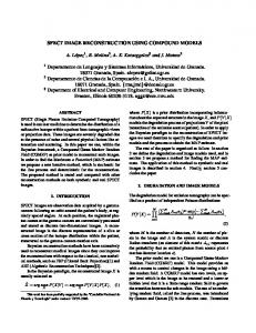
MAP Reconstruction

Mixture Decomposition

Figure 1. The alternating algorithm can be summarized in this diagram. The left side is a conventional MAP reconstruction with gamma mixture priors and the parameters provided by the right side. Given the reconstruction from the left side, then the right side becomes a mixture decomposition. Statistical image reconstruction seeks to optimize an objective function based in part on the noise model of the data. For example, since the photon emission follows a Poisson distribution, the Poisson likelihood is incorporated in the objective function for the statistical reconstruction problem. Using Bayes theory, the objective is also capable of incorporating an object constraint in the form of a penalty or prior based on some prior information about the underlying object. We are interested in two types of prior model, smoothing and pointwise priors. The smoothing priors, using assorted forms of quadratic and non-quadratic smoothing functions, force pixels values to be similar to those of neighbors.4,5 In contrast to smoothing priors, the pointwise priors have no neighbor interactions, but the estimate of each pixel is controlled by two parameters, a mean and variance. 6,7 The independent gamma prior6 is one of the pointwise priors and has many nice properties including a natural non-negativity constraint, conjugacy to the Poisson distribution, and controllable parameters of mean and variance. Using pointwise gamma priors leads to mathematical conveniences, but brings about the obvious problem of choosing the local mean and variance at each location. One possible solution is to use an initial estimate, e.g. FBP, to extract the required mean, and empirically set variance. We had proposed a joint MAP (maximum a posteriori) approach with a new prior model,1 a mixture of pointwise gamma distributions, that automatically solves the problem of computing the individual mean and variance for each element. The prior models the object as comprising a few clusters of attenuation coefficients (e.g. soft tissue, lung, bone). This model is particularly applicable to transmission tomography since the attenuation map is usually well-clustered and the approximate values of attenuation coefficients in each region are known. The overall algorithm is implemented as two alternating procedures as shown in Fig.1, a regularized likelihood reconstruction (the left-hand side) and a mixture parameter estimation (the right-hand side), which calculates the mean and variance for each location. The joint MAP reconstruction algorithm with parameter estimation can be effective, but has the problem of sensitivity to initial conditions since the overall objective is non-convex. To make it more practical, it is necessary to avoid such dependence on the initial conditions. Here, we propose the use of a deterministic annealing (DA)8 procedure to solve the problem of dependence on initial condition. The reason that DA can avoid the initial condition problem is that it tracks a solution with a computational “temperature”. At high temperature, objective is convex. As temperature is lowered, solution at high temperature is tracked. At lower temperature, we then recover the original objective, but use an initial estimate delivered by the convex high temperature objective. The DA algorithm cannot be proven to yield a global minimum of the objective, but in many applications, it leads to a robustness of the solution to variation of initial conditions. In this paper, first the transmission reconstruction problem is introduced in terms of a regularized likelihood function with independent gamma priors. A gamma mixture model prior is then described and incorporated into the reconstruction problem as a way of computing the individual parameters for the independent gamma priors. A DA 2

to appear in Proc. SPIE MI 2001

procedure is added to the regularized reconstruction processes. The schedule of the DA is then explained. Finally, we will compare the results of the joint MAP reconstruction with/without DA under many different initial conditions.

2. THEORY 2.1. Likelihood Function The transmission object of an attenuation map is denoted by vector µ with N lexicographically ordered elements µ n for each pixel n ∈ {1, .., N }. The transmission projection data is then denoted by vector g of M lexicographically ordered elements gm , where m ∈ {1, .., M } indexes the detector bins. The reconstruction problem is to reconstruct µ from the data g. The transmission projection data g follows independent Poisson distributions at each bin m, and with mean g¯m given by P (1) g¯m = um e− m Hmn µn + r¯m ,

where {um ; m = 1, .., M } are the blank scans without object in the scanner, and r¯m indicates mean background events such as scatter or randoms in PET. Note that r¯m has to be estimated before reconstruction, but this problem is not considered here. We are concerned only with the problem of low counts. We use H to denote the system matrix, which comprises elements {Hmn = lmn ; m = 1, .., M ; n = 1, .., N }, the chord length of ray m intersecting pixel n. The objective function of Poisson log likelihood for transmission tomography thus becomes X ΦL (g|µ) = {gm log(¯ gm ) − g¯m } (2) m

where constant terms have been dropped. In this paper, we use the Bayesian vocabulary of likelihood, and prior probabilities, and objective functions Φ are then logs of the associated probabilities.

2.2. Independent Gamma Priors The independent gamma prior6 takes the form p(µ|α, β)

=

N Y

n=1

αn αnαn n −1 − βn µn µα e αn n βn Γ(αn )

(3)

where α and β are vectors with components αn , βn at each pixel n. Here, Γ(x) is a gamma function. Also, αn > 1. At each pixel n, the gamma pdf controls the value (mode of pdf) to which µ n is attracted, and the weight of that attraction. It does this through its mode, βn (1 − 1/αn ), and variance, βn2 /αn . The gamma density → 0 as µ → 0, so positivity is preserved. Note that the mode of the gamma prior βn (1 − 1/αn ) is less than its mean βn . The estimate then leads to a slightly biased result. To solve this problem, we use a modified mean β n0 , βn0 =

βn αn βn = 1 − 1/αn αn − 1

(4)

2.3. Regularized Likelihood with Gamma Prior From the Bayes theorem, the maximum a posteriori reconstruction estimate of the object µ is obtained by optimizing a regularized likelihood objective Φ(µ|g) with prior (or penalty) term ΦP (µ|θ), where vector θ is the prior’s ˆ is computed by (with θ known) hyperparameter. Therefore, the MAP reconstruction µ ˆ = arg max{ΦL (g|µ) + ΦP (µ|θ)} µ µ

(5)

For the independent gamma priors, θ = (α, β), the prior term becomes ΦP (µ|α, β) =

N X

{(αn − 1) log µn −

n=1

3

αn µn } βn

(6)

to appear in Proc. SPIE MI 2001

Using 2, the final objective for the regularized likelihood with gamma priors is Φ(µ) = ΦL (g|µ) + ΦP (µ|α, β) =

X

{gm log(¯ gm ) − g¯m } +

m

N X

{(αn − 1) log µn −

n=1

αn µn } βn

(7)

ˆ by applying any suitable optimization algorithm to this One can then obtain a penalized likelihood reconstruction µ objective, which is convex and has positivity imposed directly by the gamma prior. However, it requires specifications of the 2N parameters, αn , βn , n = 1, .., N . With this strategy, one would have to thus estimate 3N parameters (N for µ, N for α, N for β) from the M measurements g. Instead, to retain the nice properties of gamma prior, we proposed a new scheme of simultaneously reconstructing the object and estimating the hyperparameters under Bayesian or penalized-likelihood principles, using gamma mixture models in computing the individual gamma parameters. The new scheme requires we estimate at most 3L + N parameters, where L ¿ N .

2.4. Joint MAP Reconstruction The joint MAP strategy is to simultaneously solve for µ as well as parameters ψ. Now we refer to ψ as the mixture parameters {π, α, β}, which will be explained further in next section. The joint MAP scheme 1 for transmission reconstruction and computing hyperparameters is ˆ = arg max p(µ, ψ|g) = arg max p(g|µ)p(µ|ψ)p(ψ) ˆ ψ µ, µ,ψ µ,ψ

(8)

where p(µ|ψ) is the proposed mixture prior with mixture hyperparameters ψ, and p(ψ) the hyperprior. In terms of objective functions, one can write the alternating algorithm as ˆ ˆ = arg max{ΦL (g|µ) + ΦP (µ|ψ)} µ µ

(9)

ˆ = arg max{ΦP (µ|ψ)} ˆ ψ ψ

(10)

ˆ as in Eq.(9) holding ψ fixed, then the parameters The tactic is to use an alternating iterative procedure, updating µ ˆ as in Eq.(10) holding µ fixed. The alternation is thus seen as an alternating ascent on the ψ variables followed by ψ ascent on the µ variables. Next, we will describe the mixture model priors.

2.5. Gamma Mixture Model as Priors Assume we are given a set of independent observations µ = {µ1 , ..., µN } and it has a mixture model of L component densities. Then it has the mixture density function p(µ|α, β, π) =

L N X Y

πa p(µn |αa , βa )

(11)

j=1 a=1

where the mixture parameters ψ = {α, β, π}, with elements {αa , βa and πa ; a = 1, .., L}, indicate the component PL parameters and mixing proportion of class a, with the constraints a=1 πa = 1, πa > 0. Note that p(µn |αa , βa ) is the conditional (gamma) density function given that µn belongs to class a.9 Here the gamma mixture component parameters (α, β) now indicate vectors of L variables (αa , βa ; a = 1, .., L). The motivation of using the mixture model is that the histogram of attenuation coefficients in an area like thorax comprises several peaks, each identified with a particular tissue type (indexed by a), i.e. soft tissue, lung and bone. A finite mixture model can account for this multimodal distribution. For the mixture model, we now need estimate at most 3L additional parameters rather than 2N . Since L is typically less than 5, our predicament is improved, however. By using the gamma mixture model prior, the prior term in Eq.(6) is now expressed as the log of Eq.(11). That is, for the alternating procedure, Eq.(10) becomes a mixture decomposition problem. There are many methods available for estimating the mixture parameters, and ML estimation via the EM (expectation-maximization) algorithm is the most popular one.10 The EM algorithm for mixture problems can also be interpreted11 as an method of coordinate descent on a particular objective in terms of an energy function. 4

to appear in Proc. SPIE MI 2001

Hence, by using the energy-based optimization scheme, there P is no E-step as needed in the EM algorithm. First, let’s define the complete data z with element zan , where a zan = 1 and 0.0 ≤ zan ≤ 1.0, Here, zan is analog and indicates a degree of membership of pixel n in class a. The energy function for the mixture model is then chosen as 11 Emix (µ|z, π, α, β) =

XX n

{zan log zan + zan log

a

1 } πa p(µn |αa , βa )

(12)

P P subject to the constraints of a zan = 1 and 0.0 ≤ zan ≤ 1.0. The first term, zan log zan can be a πa = 1, viewed as the negative of the entropy on zan , and the second term a weighted distance function between µn and subpopulation a.11 Here, the goal is to minimize the energy function, while for EM it is to maximize the likelihood. By using Lagrange multipliers and adding two constraints into the energy function, an overall mixture objective energy function is obtained, " # XX X X X 1 mix ΦP (µ|z, π, α, β) = − {zan log zan + zan log } − η( πa − 1) + κn ( zan − 1), (13) πa p(µn |αa , βa ) n a a n a P P where Lagrange multipliers η and κn are used in imposing the constraints a πa = 1 and a zan = 1. Note that we add a minus sign to the energy function to make the optimization problem a maximization one. Therefore, the mixture parameters are estimated by optimizing the mixture objective function of Eq.(13), ˆ = arg max {Φmix (µ|z, π, α, β)}. ˆ, π, ˆ α, ˆ β z P Z,π ,α,β

(14)

First, by optimizing the unconstrained objective function Eq.(13) w.r.t zan and the Lagrange multipliers κn while keeping others fixed, one can obtain a closed-form update for zˆan . Then by zeroing the first derivatives of Eq.(13) w.r.t πa and the Lagrange multiplier η, one can also get a closed-form solution for π ˆ a . The update equation for βˆa is derived by zeroing the first derivatives of the objective function w.r.t. β a . For α ˆ a , it cannot be solved explicitly and we resort to a 1-D optimization method. The final update equations for mixture parameters are π l p(µn |αal , βal ) l+1 zan = Pa l l l b πb p(µn |αb , βb ) X 1 z l+1 π ˆal+1 = N n an P l+1 l+1 n zan µj ˆ βa = P l+1 n zan X αa µn αa − log Γ(αa ) − ]. zan [(αa − 1) log µn + αa log( α ˆ al+1 = arg max αa β βa a n

(15) (16) (17) (18)

Note that l is the index for the mixture decomposition along. Later, we will use index k to indicate the overall joint MAP reconstruction. Also note that we did not describe any hyperprior terms here. However, the hyperpriors can be added easily,1 and the results follow readily. Note that the energy-based update equations lead to the same update equations as those of EM algorithms for mixture decompositions.11

2.6. Alternating Algorithms By using the mixture energy objective in the joint MAP scheme of Eq.(8), the overall objective becomes Φ(µ, π, α, β, z|g) = ΦL (g|µ) + Φmix P (µ|π, α, β, z)

(19)

with the alternating algorithm now assuming the form: ˆ k−1 , z ˆ k−1 , α ˆ k−1 , β ˆk−1 ) ˆ k = arg max ΦL (g|µ) + Φmix µ P (µ|π µ k

ˆ = arg max Φmix (µ ˆ k, z ˆk , α ˆ k, β ˆ k |π, α, β, z) π P π Z,αβ 5

(20) (21)

to appear in Proc. SPIE MI 2001

The new term, which replaces ΦΓP in (7), is given by XX αa k ˆ k |π, α, β, z) = [zan (αa − 1) log µ ˆkn − zan µ ˆ ]. Φmix P (µ βa n n a

(22)

Note that Eq.(20) is a reconstruction, and Eq.(21) a mixture decomposition that fits parameters of each class to the current histogram.

The overall reconstruction procedure, for each iteration k, turns out to alternate between MAP reconstruction (left-hand side) in Eq.(20) and mixture decomposition (right-hand side) in Eq.(21). From the comparison of the prior objective in Eq.(22) to that in Eq.(6), we can obtain the final individual hyperparameters of the independent gamma priors as a z-weighted combination of mixture class parameters, α a , βa : X αn − 1 = zan (αa − 1) (23) a

αn βn

=

X a

zan

αa . βa

(24)

2.7. Deterministic Annealing on Mixture Simulation results12,13 of the joint MAP reconstruction demonstrate its effectiveness in attenuation correction as used in the PET emission reconstruction. However, since the overall objective with gamma mixture model is nonconvex, ˆ 0 , and initial mixture it is then sensitive to the initial conditions. The initial conditions include initial image µ hyperparameters. In order to make the method more practical, it is necessary to avoid such dependence on the initial conditions. Next, we will apply a deterministic annealing procedure on the mixture decomposition. By adding the DA schedule to the mixture objective, the new objective now becomes ¸ X X X X· 1 mix − η( πa − 1) + κn ( zan − 1) T zan log zan + zan log ΦP = − k πa p(ˆ µn |αa , βa ) a n a an

(25)

where T is the DA temperature. Since the DA only has an effect on z, it changes only the final update equation on ˆ while others remain the same as in Eqs.(16)(18)(17). The new update for z an with DA turns out to be z 1

l+1 zˆan

[πa p(µn |αa , βa )] T =P 1 T b [πb p(µn |αb , βb )]

(26)

t-loop

k-loop

MAP Reconstruction

Mixture Decomposition

l-loop

Figure 2. This illustrates the t−k−l loops of the joint MAP reconstruction with DA where t indexes the temperature loop, k indexes the alternating MAP loop, and l indexes the mixture decomposition loop. (In k-loop, it has one iteration of MAP reconstruction for each k.) Therefore, the left-hand side of the alternating algorithms remains the same as in Eq.(20). But the right-hand side, the mixture decomposition, changes in the z updating equations, at each temperature T , where T decreases with its own iteration t, and follows some schedule. Hence, the temperature T is implemented as the most outer loop t as shown in Fig.2, the joint MAP iteration k lies below, and the inner most loop l is the mixture decomposition. 6

to appear in Proc. SPIE MI 2001

3. METHODS The joint MAP reconstruction has shown successful application on attenuation-corrected PET emission reconstruction.13 Here, to make it more practical, we apply the DA procedure on the right-hand side of the alternating algorithms and make it free of initial conditions. We illustrate the effectiveness of DA and compare anecdotal results of joint MAP reconstructions with/out DA under different initial conditions.

3.1. Reconstruction Details To simulate the PET imaging, we used the attenuation object as shown in Fig.3, which has only two values of narrow-beam attenuation coefficients appropriate for 511KeV, 0.095cm−1 for soft tissue and 0.035cm−1 for lung. The object comprises 128x128 pixels. We used transmission counts of 500K. The sinogram had dimensions of 129 angles by 192 detector pairs per angle. No detector effects or background effects were modeled here.

Figure 3. The attenuation object used in the simulations. To test different IC’s for joint MAP reconstructions with/out DA , we generated four IC’s from the sinogram data. The first initial estimate is an image with constant value everywhere (row 1, col 1 of Fig.4). The second initial estimate was generated by an EM-ML transmission reconstruction 14 stopped at iteration 10 (row 2, col 1 of Fig.4). A 2-iteration ML transmission reconstruction using a preconditioned conjugate gradient algorithm was used for the third initial estimate (row 3, col 1 of Fig.4), while a FBP transmission reconstruction with Hamming filter was produced for the fourth initial estimate (row 4, col 1 of Fig.4). We then used the four IC’s on the joint MAP reconstructions with and without DA. For the mixture prior, we used L = 2 (lung, soft tissue). In this study, class mean βa and complete data zan were computed by the right-hand side of the alternating algorithm, but αa was set fixed by hand empirically at an appropriate value. This is roughly equivalent to setting the smoothing parameter for the smoothing priors. The values for α a in (lung, soft tissue) for the case without DA were set at (15, 60), while for the case with DA were (50, 50). The initial condition for class mean βa were (0.028, 0.084) of (lung, soft tissue). Note that here the true class means for (lung, soft tissue) are (0.035, 0.095) at 511KeV. The initial setting of πa was not especially critical, and was easily estimated. 3.1.1. DA Scheduling The DA temperature T starts at a maximum value Tmax and decreases at a rate of ² at each temperature iteration index t. That is, for each iteration t, the DA temperature becomes T = Tmax × ²t . The maximum temperature of the DA was set at Tmax = 500, and the decreasing rate ² = 0.95. Note that Tmax should be set as large as possible and ² should be closer to 1.0. Since the estimate of πa is not critical, we dropped the update procedure for πa in the joint MAP reconstruction with DA, and set it to a uniform value of L1 .

3.2. Results The anecdotal results of the joint MAP reconstructions for 4 IC’s are shown in column 2, without DA, and column 3, with DA, of Fig.4. The reconstructions without DA display 4 different results, and thus indicate high dependence on the IC’s. Among the 4 IC’s, the 2-iteration ML initial estimate is the best IC for the case without DA. However, the reconstructions with DA illustrate nearly identical results for 4 IC’s, and thus independence on IC’s. Note that the initial value of βa is also required to be set as an IC. Here, we used the same initial estimate of the 2-iteration ML transmission reconstruction, but with a different initial value of (0.056, 0.056) for β a of (lung, soft 7

to appear in Proc. SPIE MI 2001

IC

without DA

with DA

Figure 4. This illustrates the results of joint MAP reconstructions with/out DA for different initial conditions. Column 1 illustrates four different IC’s. Columns 2 and 3 indicate joint MAP reconstructions with and without DA. Rows indicate results for different IC’s of uniform, 10 iteration of EM-ML, 2 iteration of ML, and FBP transmission reconstructions. The results show that DA is nearly independent of IC’s. The third column displays nearly identical reconstructions from the DA but still show small differences especially in the boundary pixels between lung and soft tissue. Without DA, the reconstructions differ considerably.

8

to appear in Proc. SPIE MI 2001

tissue). The fixed αa remains the same as before. The results with/out DA are shown in Fig.5. Again, the result with DA in Fig.5(b) shows the independence of IC’s but the result without DA in Fig.5(a) does not, compared to the images of col 2 and 3, row 3 of Fig.4. Thus DA adds a robustness to initial choice of β a as well as initial object estimate.

(a)

(b)

Figure 5. This illustrates the results of joint MAP reconstructions (a) with and (b) without DA at different initial value of βa compared to the results in row 3 of Fig.4. The initial estimate is the same (2-iteration ML transmission reconstruction). The result with DA again displays the same reconstruction as in Fig.4, but the one without DA has a different outcome and thus illustrates the dependence on IC’s (this time, on initial value of β a )

4. DISCUSSION AND CONCLUSION Our joint-MAP reconstruction with gamma mixture priors for low-count transmission reconstruction has proven to be effective but has the problem of sensitivity to initial conditions. Here, we have demonstrated the use of DA scheme in the joint-MAP reconstruction eliminates the dependence on the initial conditions. Basically, one can use any initial estimate, and initial values for the mixture parameters on the joint-MAP reconstruction with DA. This has the advantage of robustness. However, the use of DA brings another problem of slow reconstruction. To carefully choose the maximum DA temperature Tmax and decreasing rate ² may alleviate the problem of slow convergence. More studies are needed on this problem. The value of αa plays an important role on the final reconstruction. We found that small values of α a led to high bias and large misclassifications. The reason could be that mixture decomposition tries to fit a narrow histogram with a broader curve, and thus results a wrong mixture classifications. In particular, the attenuation object used in this simulation has two-peak histogram (extremely narrow). This can be verified by running a pure mixture decomposition simulation (not shown here) with different fitted αa from data generated αa . If the fitted value is smaller than the data generated one, mixture decomposition has difficulties of decomposing the mixture model. To make the joint-MAP reconstruction without DA produce the same good result as the one with DA, one needs to carefully choose good initial conditions, and that reduces the robustness of the method. Nevertheless, for the choice of IC, one good candidate is the FBP reconstruction. However, FBP reconstruction on a low-count data has bias and noisy spots, which would transfer into the joint-MAP reconstruction as many misclassifications (see col 2, row 4 of Fig.4). Similar results can be seen in a SAC attenuation estimate since FBP reconstruction is used in the segmentation of the SAC procedure.

ACKNOWLEDGMENTS This work is supported by grant R01-NS32879 from NIH-NINDS.

REFERENCES 1. I.-T. Hsiao, A. Rangarajan, and G. Gindi, “Joint-MAP Reconstruction/Segmentation for Transmission Tomography Using Mixture-Models as Priors”, Proc. IEEE Nuclear Science Symposium and Medical Imaging Conference, II, pp. 1689–1693, Nov. 1998.

9

to appear in Proc. SPIE MI 2001

2. J. A. Fessler, “Hybrid Poisson/Polynomial Objective Functions for Tomographic Image Reconstruction from Transmission Scans”, IEEE Trans. Image Processing, 4(10), pp. 1439–1450, Oct. 1995. 3. M. Xu, W. Luk, P. Cutler, and W Digby, “Local Threshold for Segmented Attenuation Correction of PET Imaging of the Thorax”, IEEE Trans. Nuclear Science, 41(4), pp. 1532–1537, Aug. 1994. 4. E. U. Mumcuoglu, R. Leahy, S. R. Cherry, and Z. Zhou, “Fast Gradient-Based Methods for Bayesian Reconstruction of Transmission and Emission PET Images”, IEEE Trans. Med. Imaging, 13(4), pp. 687–701, Dec. 1994. 5. J.A. Fessler, “Grouped Coordinate Descent Algorithms for Robust Edge-Preserving Image Restoration”, Proc. SPIE: Image Reconstruction and Restoration II, 3170, July 1997. 6. K. Lange, M. Bahn, and R. Little, “A Theoretical Study of Some Maximum Likelihood Algorithms for Emission and Transmission Tomography”, IEEE Trans. Med. Imaging, 6(2), pp. 106–114, June 1987. 7. J.A. Case, T.-S Pan, M.A. King, B.C. Penney, and M.S.Z. Rabin, “Reduction of truncation artifacts in fanbeam transmission imaging using a spatially varying gamma prior”, IEEE Trans. Nuclear Science, 42(6), pp. 2260–2265, Dec. 1995. 8. G. Gindi, A. Rangarajan, M. Lee, P. J. Hong, and G. Zubal, “Bayesian Reconstruction for Emission Tomography via Deterministic Annealing”, In H. Barrett and A. Gmitro, editors, Information Processing in Medical Imaging, pp. 322–338, Springer–Verlag, 1993. 9. B.S. Everitt and D.J. Hand, Finite Mixture Distributions, Chapman and Hall, 1981. 10. A. P. Dempster, N. M. Laird, and D. B. Rubin, “Maximum Likelihood Estimation from Incomplete Data via the EM Algorithm”, J. Royal Statist. Soc. B, 39, pp. 1–38, 1977. 11. R. J. Hathaway, “Another Interpretation of the EM Algorithm for Mixture Distributions”, Stat. Prob. Letters, 4, pp. 53–56, 1986. 12. I.-T. Hsiao and G. Gindi, “Comparison of Gamma-Regularized Bayesian Reconstruction to Segmentation-Based Reconstruction for Transmission Tomography”, J. Nuclear Medicine, 40, pp. 74P, May 1999. 13. I.-T. Hsiao, W. Wang, and G. Gindi, “Performance Comparison of Smoothing and Gamma Priors for Transmission Tomography”, In Proc. IEEE Nuclear Science Symposium and Medical Imaging Conference, vol. II, pp. 860–864, Oct. 1999. 14. K. Lange and R. Carson, “EM Reconstruction Algorithms for Emission and Transmission Tomography”, J. Comp. Assist. Tomography, 8(2), pp. 306–316, April 1984.

10

to appear in Proc. SPIE MI 2001