6344
IEEE TRANSACTIONS ON SIGNAL PROCESSING
Sequential Bayesian Sparse Signal Reconstruction Using Array Data Christoph F. Mecklenbräuker, Senior Member, IEEE, Peter Gerstoft, Member, IEEE, Ashkan Panahi, Student Member, IEEE, and Mats Viberg, Fellow, IEEE
Abstract—In this paper, the sequential reconstruction of source waveforms under a sparsity constraint is considered from a Bayesian perspective. Let the wave field, which is observed by a sensor array, be caused by a spatially-sparse set of sources. A spatially weighted Laplace-like prior is assumed for the source field and the corresponding weighted Least Absolute Shrinkage and Selection Operator (LASSO) cost function is derived. After the weighted LASSO solution has been calculated as the maximum a posteriori estimate at time step , the posterior distribution of the source amplitudes is analytically approximated. The weighting of the Laplace-like prior for time step is then fitted to the approximated posterior distribution. This results in a sequential update for the LASSO weights. Thus, a sequence of weighted LASSO problems is solved for estimating the temporal evolution of a sparse source field. The method is evaluated numerically using a uniform linear array in simulations and applied to data which were acquired from a towed horizontal array during the long range acoustic communications experiment. Index Terms—Bayesian estimation, sequential estimation, sparsity, weighted LASSO.
I. INTRODUCTION
C
OMPRESSIVE sensing and sparse reconstruction is widely used, but their sequential use have received little attention. In a Bayesian framework, the sparseness constraint is obtained using a Laplace-like prior which give rise to the constraint. In the present contribution the focus is on developing a Bayesian sequential sparse approach by enforcing the prior at each step to be Laplace-like. Since the late nineties, numerous papers have appeared in the areas compressive sensing and sparse reconstruction which employ the penalization by a -norm to promote sparsity of the solution, e.g., [1]–[6]. Excellent books on the topic are available [7], [8]. The least absolute shrinkage and selection Manuscript received March 18, 2013; revised July 31, 2013; accepted September 12, 2013. Date of publication September 20, 2013; date of current version November 14, 2013. The associate editor coordinating the review of this manuscript and approving it for publication was Prof. Maria Sabrina Greco. The work was funded by Grant ICT08-44 of Wiener Wissenschafts—Forschungs–und Technologiefonds, National Science Foundation EAR-0944109, and the Swedish Research Council (VR). C. F. Mecklenbräuker is with the Institute of Telecommunications, Vienna University of Technology 1040 Vienna, Austria (e-mail:
[email protected]). P. Gerstoft is with the University of California San Diego, La Jolla, CA 92093-0238 USA (e-mail:
[email protected]; website: http://www.mpl.ucsd. edu/people/pgerstoft). A. Panahi and M. Viberg are with the Signals and Systems, Chalmers University of Technology, Göteborg S-41296, Sweden (e-mail:
[email protected];
[email protected]). Color versions of one or more of the figures in this paper are available online at http://ieeexplore.ieee.org. Digital Object Identifier 10.1109/TSP.2013.2282919
operator (LASSO) is a least squares regression constrained by an -bound of the solution [1]. It is well-known that the LASSO sets many regression coefficients to zero favoring sparse solutions. Research on compressive sensing and sparse reconstruction has focused largely on batch processing. However, many practical settings require the online estimation of sparse signals from noisy data samples that become available sequentially [9]–[11]. Angelosante et al. proposed time-recursive algorithms for the estimation of time-varying sparse signals from observations obeying a linear model, and become available sequentially in time [10]. Their time-weighted LASSO is an -norm regularized Recursive Least Squares algorithm. Eiwen et al. [11] proposed a sequential compressive channel estimator which is based on modified compressed sensing, which assumes that a part of the signal support is known a priori. The resulting compressive channel tracker uses a modified version of the orthogonal matching pursuit algorithm. An iterative pursuit algorithm is developed in [12] that uses sequential predictions for dynamic compressive sensing. It incorporates prior information using linear MMSE reconstruction. Here, we extend the Bayesian approach [13]–[15] to sequential Maximum A Posteriori (MAP) estimation for sparse signal reconstruction in a problem setting that is similar to [10]. First the LASSO cost function is generalized by weighting the regularization parameters. This allows to update the prior adaptively based on the past history of observations. Based on ideas in [16], we approximate a sequential MAP filter which preserves sparsity in the source field estimates. Two types of approximations are derived in Sections III-D and III-E and their behavior is compared in numerical examples. It is implemented by sequentially minimizing adaptively weighted LASSO cost functions using a single new measurement snapshot in each time step. The theory is formulated so that it can be applied to sparse source field estimation in higher spatial dimensions. We have earlier demonstrated the sequential approach for a two dimensional array, where an earthquake rupture process evolves sequentially with sparse locations in both time and two dimensional space [17]. High resolution earthquake location has been obtained using compressive sensing [18]. The advantages of the sparse formulation for source localization and direction of arrival (DOA) estimation are: • Numerical simulations indicate that it is a high-resolution method [3]. • There is no need to estimate the cross-spectral density matrix. Only one snapshot is needed. Eigenvalue based high-
1053-587X © 2013 IEEE
MECKLENBRÄUKER et al.: SEQUENTIAL BAYESIAN SPARSE SIGNAL RECONSTRUCTION USING ARRAY DATA
resolution methods require a full or nearly full Cross Spectral Density Matrix (CSDM). • As new information becomes available, the confidence in the solution is build up and the trajectories are updated. • The solution is presented in terms of a sparsifying Laplacian distribution which can then be used as a prior in the sequential processing. Relative to more general solutions like particle filters, the solution requires just one parameter per possible source location. II. ARRAY DATA MODEL AND PROBLEM FORMULATION Let be a set of hypothetical source locations on a given fixed grid. Further, let be the associated complex-valued source vector at time step and frequency . We observe time-sampled waveforms on an array of sensors which are stacked in a vector. We obtain the following linear model which relates the short-time Fourier transformed sensor array output at time step and at frequency to the source vector , (1) The th column of the transfer matrix is the array steering vector for hypothetical source location . The transfer matrix is constructed by sampling all possible source locations, but only very few of these can correspond to real sources. Therefore, the dimension of is with and is sparse. In our setting, the number of hypothetical source locations is much larger than the number of sensors , i.e., and the linear model (1) are underdetermined. We model the th element of by . Here is the traveltime from hypothetical location to the th sensor element of the sensor array. The additive noise vector is assumed to be spatially uncorrelated and follows the zero-mean complex normal distribution with diagonal covariance matrix . Further, the noise is assumed to be uncorrelated across time and frequency. The history of all previous array observations is summarized in . Given the history and the new data , we seek the maximum a posteriori (MAP) source estimate under a sparsity constraint. To reconstruct a physically meaningful source vector , we enforce its sparsity through the introduction of a prior probability density on which promotes sparsity. A widely used sparseness prior is the Laplace probability density [14], [19] which puts a higher probability mass than the normal distribution both for large and small absolute deviations. The prior distribution for each is assumed to follow a Laplace distribution with hyperparameter , condensed in vector . A time-recursive expression of the sparse MAP source estimate at step is obtained using a sequential Bayesian sparse update rule
6345
sequential information from each step, and not the extracted parameters as is customary in sequential filtering [20]. Since the conditional distribution for given follows a Gaussian (3) it is not given that the posterior will be Laplacelike. As the posterior for time step is used as a prior in the next time step it is required to approximate the posterior with a Laplace-like distribution. The hyperparameter is determined by matching either the probabilities for large source amplitudes (i.e., the tail of the distribution, see Section III-D) or the expected source amplitudes (Section III-E). III. BAYESIAN FORMULATION For the linear model (1), we arrive at the following conditional probability density for the single-frequency observations given the source vector , (3) where is the -norm. We assume a multivariate complex Laplace-like probability density [21] for the source vector at step , conditioned on the history , (4) is the complex source signal at step and hypothetical source location . Note that (4) defines a joint distribution for and at step for all . The associated hyperparameters model the prior knowledge on the occurrence of a source at step , at location . Taking the logarithm gives
(5) For the posterior probability density function (pdf) , we use Bayes’ rule to obtain the weighted LASSO cost function to be minimized, cf. Equation (6) in [16]:
(6) (7)
L in which the notation L
is introduced and
(2)
(8)
Where the function will be derived in the following. In addition to , the hyperparameter for the prior distribution for the next time step is computed. Due to the sparsity constraint it is necessary to let the hyperparameters carry the
Minimizing the weighted LASSO cost function (7) with refor given and , gives spect to the MAP source estimate . The in (6) is the element-wise
6346
IEEE TRANSACTIONS ON SIGNAL PROCESSING
(Hadamard–) product, making it clear that this is a cost function promoting sparse solutions in which the constraint is weighted by giving every source amplitude its own hyperparameter . The minimization of (7) constitutes a convex optimization problem.
(7) around the MAP We expand the LASSO cost function L source estimate using (15) and then (10):
L
A. Posterior Probability Density The purpose of this section is deriving an expression for the posterior pdf . We distinguish the variable , a free variable for , and , the MAP source estimate which is treated as constant. at step is introduced as the set The set of active indices is non zero, i.e., of such that
(16) L
(9) The true and the estimated source amplitude vectors are related by the source vector error :
(17)
where we introduced the polar representations,
(10)
(18)
using the active indices for for
(11)
The log-likelihood function (7) is expanded
is the magnitude of the projection of the normalized residual vector onto the th array steering vector. for . Equation (17) shows By Theorem 1, that the posterior pdf depends on both the unknown source magnitudes and phases . In the Section III-B, an approximate marginal posterior pdf for the source magnitudes is derived. This allows to approximate the next MAP estimate as the minimizer of an updated weighted LASSO cost function. B. Marginalization With Respect to Source Phases
(12) where we separated the sum and used (11). The sum over is simplified by the following Theorem 1: For given weighting , the MAP source estito (7) is characterized by (cf. mate (minimizing solution) [16]) (13a) (13b) with the normalized residual vector
From (4), it follows that the prior for the source phases . We regard is i.i.d. uniformly distributed on the phases as nuisance parameters and marginalize L in (7) inserting (17) and integrating the phases out. The source vector errors are assumed small and is neglected in (17). Assuming the errors to be small is common in sequential methods. For example the Extended Kalman Filter (EKF) also assumes small errors so that the parameter estimate remains Gaussian. As demonstrated in the sequel, we use this approximation so that the posterior remains Laplacian. This is motivated by the assumption that the posterior pdf is concentrated around its peak point . Using (17), the approximate marginal posterior pdf depends solely on the source magnitudes
(14) L
The proof is in Appendix A. Continuing from (12), gives L
(15)
(19)
MECKLENBRÄUKER et al.: SEQUENTIAL BAYESIAN SPARSE SIGNAL RECONSTRUCTION USING ARRAY DATA
where ,
is the vector of source magnitudes with elements is a normalization constant defined by
For amplitude
6347
we get (25)
L
The asymptotic expansion (24)–(25) has a small approximation error for . Taking the logarithm analogously to (5), gives
for for (20) is the modified Bessel funcand tion of first kind and zero order, cf. [23]:9.6.16. To assess the quality of the approximation in (19), we use the first order Taylor expansion in the vicinity of the MAP estimate , (21)
(26) (Theorem 1) and is large, we neglect and in (26). Finally, all these steps and approximations give the posterior weighted -penalty Since
(27) In (19), only the constant term was retained and the quality of the approximation depends on the magnitude of . The approximate marginal pdf (19) becomes improper as because it cannot be normalized on the half line in the limit . This difficulty occurs when the index becomes active (see Section III-C). Its form is not Laplacelike (4) and we develop two types of approximations for fitting the posterior distribution at time step to a Laplace-like prior distribution for time step in the following Sections III-D and III-E.
The weight reduces to zero when index becomes active (see Section III-C ). The first line in (28) is always positive as .
C. Active Indices
E. Mean Fit of Laplace-Like Distribution
To estimate the posterior distribution for the active indices we use (19). For any given , the Laplace-like pdf (4) favors a model with small source amplitude . In the limiting case , however, the Laplace-like pdf approaches a uniform pdf for the source amplitude which cannot be normalized. We express this informally as
Alternatively to the approach in Section III-D, the expected source amplitudes for the assumed the Laplace-like distribution (4) can be fitted to the expected posterior source amplitudes.
(22)
Comparison with (4) and combination with (23) shows that this translates to the posterior weight vector with elements for for
(28)
(29)
Proceeding from (19) for
, this gives
has become active in the current Thus, when some index time step there will be no constraint on the corresponding amplitude and we define the posterior hyperparameter
(30) (31)
(23) Note that this model has no information to see how likely an active index is to become inactive. D. Asymptotic Fit of Laplace-Like Distribution Here we are concerned with the for the inactive indices . The for any conveys prior information about how likely the index is to transition to the set of active indices at the next time step . The approximate marginal pdf (19) is close to Laplace-like (4) in terms of asymptotic behavior for large values of . The MAP estimate is sparse and many , but the variables can take any value. In this section, is assumed large. The first-order asymptotic expansion is used, (24)
For a Laplace-like distribution, (32) Combining (31) and (32) gives the elements of the posterior weight vector for . The corresponding elements for are obtained in the limit consistent with (23). The posterior weight vector becomes for for
(33)
For , the weight reduces to zero when index becomes active. The posterior weight according to (28) is always smaller than posterior weight (33) for because for
6348
IEEE TRANSACTIONS ON SIGNAL PROCESSING
Fig. 1. Number of active indices versus the regularization parameter example in Section VI.
for the
by Theorem 1. We choose (33) rather than (28), because the weighting in the cost function (6) will then play a stronger role. IV. SIMPLE SOURCE MOTION MODEL After having estimated the posterior with elements defined by (33), the next step is to predict for the Laplace-like prior (4) at time step . Time-varying source signal estimates are obtained by varying the active set (creating new active indices as well as annihilating old ones). Here, a very simple random walk model is assumed: A source occurring at location at time step is either inherited from the previous time step with probability or newly generated from an unweighted (uninformed) Laplace-like prior with parameter with probability . Thus, we define the hyperparameter for time step ,
The solution of (35) evolves with , due to the uniform continuity of the cost. Furthermore, for sufficiently large , . Thus, a solution with active indices is found by pursuing the continuum from a large . The evolution of from large to smaller values is segmented into intervals for , in which the set of active indices is constant, for corresponds to . Varying within an interval changes just for the active indices . Each interval has an end-point at a candidate point , where the active set changes by including or deleting an element (potentially multiple elements). Creation is defined as including an index into if as decreases below . Vice versa, annihilation is the process of deleting an index as with decreasing . Due to the (rather unlikely) possibility of annihilation, the number of active indices can be less than for . The sequence of with source amplitudes is found using the optimality conditions in Theorem 1. Starting from large, in the first interval , . Then, is the smallest value, for which Theorem 1 is satisfied with :
(36) . Recalling Theorem 1 The LASSO is next solved for with a given active set from the previous candidate solution , the next candidate point is the smallest with the active indexes unchanged, i.e.,
(34) is the all-1 vector. plays a role where which is similar to the process noise covariance in the Kalman filter, see Section VI. If is large then will be close to one. Then, the history has only little influence on the future estimate . Conversely, for a smaller , the adaptivity of the weighting through the posterior (28) will be more influential to the future sequential estimates. V. IMPLEMENTATION OF
USING LASSO PATH
We define the positive parameter and the vector of non-negative weighting coefficients via , equivalently . Thus the weights are obtained by the previous data and the source model and normalized so that . For the data the source vector is found by minimizing L
(35)
The optimization (35) is convex and is solved assuming a fixed number of sources . However, is unknown and adjusted to reach a desired number of active indices as described below. The weighted complex-valued LASSO is based on solving LASSO by homotopy [16], [22], as indicated in Fig. 1.
(37) where set of
is the LASSO solution for given active indexes in the interval
and :
is the (38)
, its Moore-Penrose pseudoinThe contracted dictionary verse , contracted source amplitudes , and contracted phase-weighted weights are defined by (39) (40) (41) (42) defines the projection onto the orThe projection matrix thogonal complement of the range of , (43) . The following Theorem 2 is a unitary basis of the range of provides an approximate solution to the minimization problem
MECKLENBRÄUKER et al.: SEQUENTIAL BAYESIAN SPARSE SIGNAL RECONSTRUCTION USING ARRAY DATA
6349
tially for all time steps with the implementation given in Table I with . We use synthetic data on a uniform linear array with elements with half-wavelength spacing and using 50 snapshots sequentially . The traveltime for plane waves impinging on the th sensor is modeled as
TABLE I SEQUENTIAL BAYESIAN SPARSE SIGNAL RECONSTRUCTION.
(50) for a hypothetical source at direction of arrival with and . The simulated scenario has far-field sources modeled as emitting plane waves (1). The uncorrelated noise is , i.e., power. Eight sources are stationary at degrees relative to endfire with constant power levels (PL) . The moving source starts at 65 and moving /snapshot and has a power level of . A. Beamforming (37) for a given set of active indices. The approximation is based on the assumption that the vector (42) is constant inside the interval . Equivalently, the phase angles of all elements of are assumed to be constant which is a first order approximation in . Theorem 2: The approximate solution to (37) is given by (44) where the creation
and annihilation
are
(51) (45) (46)
where
In beamforming the Cross Spectral Density Matrix (CSDM) is estimated based on all snapshots for . The CSDM estimate is singular as it is snapshot deficient, with at least eigenvalues equal zero. For conventional beamforming, the resolution is not sufficient to separate all the sources (Fig. 2). To numerically stabilize the matrix inversion in the adaptive beamforming, diagonal loading is applied at a level of relative to the sum of the eigenvalues. The stabilized beamformer output for a given steering vector is
is defined in Appendix C, and (47) (48)
is the bias-corrected estimate. The proof is in Appendix B. The implementation of the sequential Bayesian sparse signal reconstruction update in (2) is given concisely in Table I. Line 8 “Define active set” is implemented with a numerical peak finder and subsequent thresholding. Note the bias correction step in line 13 “choice 2” using just the active indexes [30]: (49) VI. NUMERICAL EXAMPLE In this section we investigate the performance of the proposed sequential sparse estimation procedure using computer simulations. For the sequential Bayesian sparse signal reconstruction, we initialize the prior vector with all ones: all hypothetical source locations have the same prior. We then apply (2) sequen-
For the stationary case (Fig. 2(a)), the conventional beamformer, in (51), resolves all 8 sources whereas the Minimum Variance Distortionless Response (MVDR) , just resolves 6 sources. For this scenario, we observe that above beamforming finds the source location well for the stationary case (Fig. 2(a)), but the moving source masks the stationary source at (Fig. 2(b)). The observed bias in the power estimate for the MVDR is due to the snapshot deficient CSDM [24]. More advanced adaptive beamforming might be able to better estimate the source locations in this scenario with higher time resolution, e.g., the multi-rate adaptive beamforming [25], [26]. Multi-rate beamforming uses long time averages to produce the MVDR steer vectors and shorter averages for the data CSDM. It was introduced to track a stable signal in the presence of dynamic interferers [25]. In contrast, the sparse localization works directly with a single snapshot optimization (7) giving higher time-resolution. Successive snapshot localizations then include the information carried forward from previous localizations via the prior and the hyperparameters. This enables finding lower powered sources than if each snapshot was used independently. B. Sequential LASSO Going down the LASSO path, Section V, is computationally demanding, especially for the 9 sources involved in the
6350
Fig. 2. MVDR and conventional beamforming for the a) stationary sources (*), and b) stationary (*) and moving (o) sources for the 50 snapshot observation period.
studied scenario. Since the noise level is constant over time, the should not change much. It is not necessary going down the full LASSO path. Therefore, each iteration is started at a slightly larger than the expected final . Assuming that the active indices do not change, the second term in (35) is proportional to . We use for and for . For a given value of , the convex optimization (35) is solved using CVX [27]–[29]. We carry out the simulations with the mean fitting approach in Section III-E which corresponds to “choice 4” in line 14 of Table I. 1) Stationary Sources: The posterior weights defined by (33) are updated after each step and used as prior information to the following snapshot forming the sequential estimation approach. The non-sequential LASSO results shown in Fig. 3(a) show more variation than those from the proposed sequential Bayesian sparse signal reconstruction shown in Fig. 3(b). The constraint in (7) that sparsifies the solution causes the power estimates (peak of solid in Fig. 3(a)) to be underestimated especially for the low-power sources (e.g., and 99 ). Using the unbiased estimate (choice 2 in line 13 of Table I) gives powers within 3 dB of the correct ones. The posterior weights show how the solution is being guided towards the solution of the active indices in the next step. 2) Moving Sources: For a moving source scenario (Figs. 5 and 6), it will be difficult observing the stationary sources using beamforming. Since the proposed approach works directly on a
IEEE TRANSACTIONS ON SIGNAL PROCESSING
Fig. 3. Track over 50 time steps for the 8 stationary sources (dots) for a) non. Background sequential LASSO and b) sequential LASSO with (color, dB) shows the conventional beamformer power.
Fig. 4. a) Output of the sparse optimization (8, solid) with unbiased (o) and true (*) source power. b) The posterior weights for
. The .
snapshot, there is sufficient time resolution to track both moving and stationary sources, cf. Fig. 5(a). The temporal evolution of the weights is shown in Fig. 6. The weights for the asymptotic fitting technique in Section III-D are
MECKLENBRÄUKER et al.: SEQUENTIAL BAYESIAN SPARSE SIGNAL RECONSTRUCTION USING ARRAY DATA
Fig. 7. Evolution of posterior weights for (red), posterior at (blue), and posterior at
Fig. 5. Track for or the 8 stationary and 1 moving source sources (dots) using b) . Background color shows sequential LASSO with a) the conventional beamformer power (dB).
6351
. Prior at (green).
Figs. 6(c) and 6(d). It is clearly seen that the contrast between the weights for active and inactive indices is much larger. The value of determines how long the weight will remember a track, the non-sequential LASSO results are obtained with in (34). A large causes the weights to faster forget a previously estimated source position (Figs. 6(a) and 6(c) ) and gives more stable track estimates (Fig. 5(a) than for the smaller . The weights for the small are shown in Figs. 6(b)–6(d) and the corresponding sequential Bayesian sparse signal reconstruction in Fig. 5(b). A small results in a longer memory as seen in Figs. 6(b) and 6(d) which is beneficial for the sparse reconstruction of static source scenarios. From Fig. 7 it is observed that the posterior weights become close to zero near the active indices. The weights have a broader valley near endfire where the resolution cells are larger. As the moving source moves from 65 to 75 the weights for the corresponding set of source locations shift. VII. EXPERIMENT
Fig. 6. Evolution of posterior weights versus , left: Asymptotic fitting in a) and c). Small using (25) and right: mean fitting using (31). Large in b) and d).
shown in Figs. 6(a) and 6(b). For the asymptotic fitting technique, the difference in the weights between active indices and inactive ones is rather small. On the other hand, the weights for the mean fitting technique in Section III-E are shown in
The data is from a towed horizontal array during the long range acoustic communications (LRAC) experiment [32], [33] from 10:00–10:13 UTC on 16 September 2010 in the NE Pacific in 5-km water depth. Other data periods yield similar results to those shown here. The array was towed at 3.5 knots at a depth of 200 m. The data were sampled at 2000 Hz using a nested array with each configuration having 64 channels [34] with the ultra low frequency (ULF) array hydrophone spacing 3 m . Each 4 s snapshot was Fourier transformed with samples without overlapping snapshots. The beamformed time series, Fig. 8(a), is based on single snapshots and performed at one quarter wavelength element spacing, i.e., 125 Hz. The broad arrival at 150–165 is from the towship R/V Melville (180 is forward looking). Apparently, the two arrivals at 45 and 60 come from distant transiting ships, although a log of ships in the area was not kept. Overall, the beam time series shows little change with time. The sparse sampling was performed assuming discrete signals and for sequential processing . Fig. 8(b) shows the non-sequential estimates, while the discrete features are well-captured with the processing, there are
6352
IEEE TRANSACTIONS ON SIGNAL PROCESSING
global minimum L the th element of
. For an infinitesimal change , we have
at
L (52) The variations in L at the global minimum satisfy L for every and . The minimality condition is satisfied for if and only if (53a) Alternatively, if
then (53b)
APPENDIX B The proof of Theorem 2 proceeds similar to Appendix B in [22]. The aim is to find the next singular point defined in (37). We rewrite the minimality condition (53a) as (54) This is solved by (55) Fig. 8. Real data example. a) Beamformer output. Tracks for 10 sources (dots) . using b) non-sequential LASSO and c) sequential LASSO with Background color shows the conventional beamformer power (dB).
It is assumed that the phase of the solution is approximately constant in one -interval [16]. Then also is approximately constant for all and depends approximately linearly on . Then, we have
significant fluctuations in the estimates from each snapshot. This is stabilized when using the sequential processing, Fig. 8(c). (56)
VIII. CONCLUSION A sequential weighted LASSO problem formulation is used to estimate the spatiotemporal evolution of a sparse source field from observed samples of a wave field. The prior is adapted based on the past history of observations. A sequential MAP filter is derived which preserves sparsity in the source field estimates by enforcing the priors at each estimation step to be Laplacian. The sequential information is carried in the hyperparameters. With a uniform linear array it is demonstrated that the proposed sequential Bayesian sparse signal reconstruction obtains high resolution in both time in space relative to adaptive beamforming. Using towed array data, the estimated tracks become more stable with the sequential estimation. APPENDIX A The proof of Theorem 1 is similar to Appendix A in [22], see also [31]. Suppose the active set in (7) is given by at the
is the orthogonal projection matrix defined in (43). where For the creation case, according to (37) and (56), is the smallest value, for which (57) for every index . This implies that the set of positive solutions of
is the largest value in
(58) for every , which is solved by the -function in Appendix C. For the annihilation case, (37) and (55) is combined. After defining and (47)–(48), we express (55) as (59)
MECKLENBRÄUKER et al.: SEQUENTIAL BAYESIAN SPARSE SIGNAL RECONSTRUCTION USING ARRAY DATA
Due to (37) annihilation occurs when , which gives for some . Thus, is the maximum of such annihilation points. This completes the proof. APPENDIX C In (45), the function is introduced. The real-valued function of complex numbers is defined as the positive root of . The resulting quadratic equation is (60) Its roots are (61) If
then
else
.
ACKNOWLEDGMENT The authors like to thank Florian Xaver for valuable discussions and comments on the manuscript. REFERENCES [1] R. Tibshirani, “Regression shrinkage and selection via the LASSO,” J. Roy. Statist. Soc. B, vol. 58, no. 1, pp. 267–288, 1996. [2] I. F. Gorodnitsky and B. D. Rao, “Sparse signal reconstruction from limited data using FOCUSS: A re-weighted minimum norm algorithm,” IEEE Trans. Signal Process., vol. 45, no. 3, pp. 600–616, 1997. [3] D. M. Malioutov, C. Müjdat, and A. S. Willsky, “A sparse signal reconstruction perspective for source localization with sensor arrays,” IEEE Trans. Signal Process., vol. 53, no. 8, pp. 3010–3022, Aug. 2005. [4] E. J. Candès, J. Romberg, and T. Tao, “Robust uncertainty principles: Exact signal reconstruction from highly incomplete frequency information,” IEEE Trans. Inf. Theory, vol. 52, no. 2, pp. 489–509, Feb. 2006. [5] D. Donoho, “Compressed sensing,” IEEE Trans. Inf. Theory, vol. 52, no. 4, pp. 1289–1306, Apr. 2006. [6] R. G. Baraniuk, “Compressive sensing,” IEEE Signal Process. Mag., vol. 24, no. 4, pp. 118–120, Jul. 2007. [7] M. Elad, Sparse and Redundant Representations: From Theory to Applications in Signal and Image Processing. New York, NY, USA: Springer, 2010. [8] Y. C. Eldar and G. Kutyniok, Compressed Sensing: Theory and Applications. Cambridge, U.K.: Cambridge Univ. Press, 2012. [9] D. M. Malioutov, S. Sanghavi, and A. S. Willsky, “Sequential compressed sensing,” IEEE J. Sel. Top. Signal Process., vol. 4, pp. 435–444, 2010. [10] D. Angelosante, J. A. Bazerque, and G. B. Giannakis, “Online adaptive estimation of sparse signals: Where rls meets the -norm,” IEEE Trans. Signal Process., vol. 58, no. 7, pp. 3436–3447, 2010. [11] D. Eiwen, G. Tauböck, F. Hlawatsch, and H. G. Feichtinger, “Compressive tracking of doubly selective channels in multicarrier systems based on sequential delay-Doppler sparsity,” in Proc. Int. Conf. Acoust., Speech, Signal Process. (ICASSP), Prague, Czech Republic, May 2011, pp. 2928–2931. [12] D. Zachariah, S. Chatterjee, and M. Jansson, “Dynamic iterative pursuit,” IEEE Trans. Signal Process., vol. 60, no. 9, pp. 4967–4972, Sep. 2012. [13] D. P. Wipf and B. D. Rao, “An empirical Bayesian strategy for solving the simultaneous sparse approximation problem,” IEEE Trans. Signal Process., vol. 55, no. 7, pp. 3704–3716, Jul. 2007. [14] S. Ji, Y. Xue, and L. Carin, “Bayesian compressive sensing,” IEEE Trans. Signal Process., vol. 56, no. 6, pp. 2346–2356, Jun. 2008. [15] S. D. Babacan, R. Molina, and A. K. Katsaggelos, “Bayesian compressive sensing using Laplace priors,” IEEE Trans. Image Process., vol. 19, no. 1, pp. 53–63, Jan. 2010.
6353
[16] A. Panahi and M. Viberg, “Fast LASSO based DOA tracking,” presented at the 4th Int. Workshop Comput. Adv. Multi-Sensor Adap. Process. (IEEE CAMSAP), Puerto Rico, San Juan, Dec. 2011. [17] P. Gerstoft, C. F. Mecklenbräuker, and H. Yao, “Bayesian sparse sensing of the japanese 2011 earthquake,” in Proc. Asilomar Conf. Signals, Syst., Comput., Pacific Grove, CA, USA, Nov. 4–7, 2012. [18] H. Yao, P. Gerstoft, P. M. Shearer, and C. F. Mecklenbräuker, “Compressive sensing of Tohoku-oki M9.0 earthquake: Frequency-dependent rupture modes,” in Geophys. Res. Lett., 2011, vol. 38, p. L20310. [19] J. M. Bernardo and A. F. M. Smith, Bayesian Theory. New York, NY, USA: Wiley, 1994. [20] B. Ristic, S. Arulampalam, and N. Gordon, Beyond the Kalman Filter: Particle Filters for Tracking Applications. Boston, MA, USA: Artech House, 2004. [21] Z. He, S. Xie, S. Ding, and A. Cichocki, “Convolutive blind source separation in the frequency domain based on sparse representation,” IEEE Trans. Audio, Speech, Lang. Process., vol. 15, no. 5, pp. 1551–1563, Jul. 2007. [22] A. Panahi and M. Viberg, “Fast candidate points selection in the LASSO path,” IEEE Signal Process. Lett., vol. 19, no. 2, pp. 79–82, Feb. 2012. [23] Handbook of Mathematical Functions With Formulas, Graphs, and Mathematical Tables, M. Abramowitz and I. A. Stegun, Eds. New York, NY, USA: Dover, Dec. 1972, 10th printing with corrections. [24] H. C. Song, W. A. Kuperman, W. S. Hodgkiss, P. Gerstoft, and J. S. Kim, “Null broadening with snapshot-deficient covariance matrices in passive sonar,” IEEE J. Ocean. Eng., vol. 28, no. 2, pp. 250–261, Apr. 2003. [25] H. Cox, “Multi-rate adaptive beamforming (MRABF),” in Proc. Sensor Array Multichannel Signal Process. Workshop, Boston, MA, USA, Mar. 16–17, 2000, pp. 306–309. [26] J. Traer and P. Gerstoft, “Coherent averaging of the passive fathometer response using short correlation time,” J. Acoust. Soc. Amer., vol. 130, no. 6, pp. 3633–3641, Dec. 2011. [27] M. Grant and S. Boyd, CVX:Matlab software for disciplined convex programming, ver. 1.21, Apr. 2011 [Online]. Available: http://cvxr. com/cvx [28] M. Grant and S. Boyd, “Graph implementations for nonsmooth convex programs,” in Recent Advances in Learning and Control. New York, NY, USA: Springer-Verlag Ltd., 2008, pp. 95–110. [29] S. P. Boyd and L. Vandenberghe, Convex Optimization. Cambridge, U.K.: Cambridge Univ. Press, 2004, ch. 1–7. [30] M. A. T. Figueiredo, R. D. Nowak, S. J. Wright, and J. Stephen, “Gradient projection for sparse reconstruction: Application to compressed sensing and other inverse problems,” IEEE J. Sel. Topics Signal Process., vol. 1, no. 4, pp. 586–597, Dec. 2007. [31] M. R. Osborne, B. Presnell, and A. Turlach, “On the LASSO and its dual,” J. Comput. Graph. Statist., vol. 9, no. 2, pp. 319–337, Feb. 2000. [32] H. C. Song, S. Cho, T. Kang, W. S. Hodgkiss, and J. R. Preston, “Longrange acoustic communication in deep water using a towed array,” J. Acoust. Soc. Amer., vol. 129, no. 3, pp. EL71–EL75, Mar. 2011. [33] P. Gerstoft, R. Menon, W. S. Hodgkiss, and C. F. Mecklenbräuker, “Eigenvalues of the sample covariance matrix for a towed array,” J. Acoust. Soc. Amer., vol. 132, no. 4, pp. 2388–2396, Oct. 2012. [34] K. M. Becker and J. R. Preston, “The ONR five octave research array (FORA) at penn state,” in Proc. IEEE OCEANS, Sep. 22–26, 2003, vol. 5, pp. 2607–2610.
Christoph F. Mecklenbräuker (S’88–M’97– SM’08) received the Dipl.-Ing. degree in electrical engineering from Technische Universität Wien, Austria, in 1992 and the Dr.-Ing. degree from Ruhr-Universität Bochum, Germany, in 1998. His doctoral dissertation received the Gert-Massenberg Prize in 1998. He was with Siemens, Vienna, from 1997 to 2000. From 2000 to 2006, he was senior researcher with the Forschungszentrum Telekommunikation Wien (FTW), Austria. In 2006, he joined the Institute of Telecommunications as full professor with the Technische Universität Wien, Austria. Since 2009 he leads the Christian Doppler Laboratory for Wireless Technologies for Sustainable Mobility. His research interests include waves, sparsity, vehicular connectivity, ultrawideband radio, and MIMO-techniques. Dr. Mecklenbräuker is a member of the IEEE Signal Processing, Antennas and Propagation, and Vehicular Technology Societies, VDE and EURASIP.
6354
Peter Gerstoft (M’13) received the Ph.D. from the Technical University of Denmark, Lyngby, Denmark, in 1986. From 1987–1992 he was with Ødegaard and Danneskiold-Samsøe, Copenhagen, Denmark. From 1992–1997 he was at Nato Undersea Research Centre, La Spezia, Italy. Since 1997, he has been with the Marine Physical Laboratory, University of California, San Diego. His research interests include modeling and inversion of acoustic, elastic and electromagnetic signals. Dr. Gerstoft is a Fellow of Acoustical Society of America and an elected member of the International Union of Radio Science, Commission F.
Ashkan Panahi (S’11) received his BSc degree in electrical engineering from Iran University of Science and Technology (IUST) in 2008. He also received his MSc degree in 2010 in the field of communication Eng. from Chalmers University, Sweden, where he is currently pursuing his PhD studies. Being with the signal processing group, signals and systems department, his main research interest includes estimation and inverse problems, sparse techniques and information theory. His current research concerns the application of sparse techniques to the sensor array problems. Ashkan Panahi has been a student member of IEEE since 2011.
IEEE TRANSACTIONS ON SIGNAL PROCESSING
Mats Viberg (S’87–M’89–SM’95–F’03) received the PhD degree in Automatic Control from Linköping University, Sweden in 1989. He has held academic positions at Linköping University and visiting Scholarships at Stanford University and Brigham Young University, USA. Since 1993, Dr. Viberg is a professor of Signal Processing at Chalmers University of Technology, Sweden. During 1999–2004 he served as Department Chair. Since May 2011, he holds a position as First Vice President at Chalmers University of Technology. Dr. Viberg’s research interests are in Statistical Signal Processing and its various applications, including Antenna Array Signal Processing, System Identification, Wireless Communications, Radar Systems and Automotive Signal Processing. Dr. Viberg has served in various capacities in the IEEE Signal Processing Society, including chair of the Technical Committee (TC) on Signal Processing Theory and Methods (2001–2003), vice-chair (2009–2010) and chair (2011–2012) of the TC on Sensor Array and Multichannel, Associate Editor of the Transactions on Signal Processing (2004–2005), member of the Awards Board (2005–2007), and member at large of the Board of Governors (2010-). Dr. Viberg has received 2 Paper Awards from the IEEE Signal Processing Society (1993 and 1999 respectively), and the Excellent Research Award from the Swedish Research Council (VR) in 2002. Dr. Viberg is a Fellow of the IEEE since 2003, and his research group received the 2007 EURASIP European Group Technical Achievement Award. In 2008, Dr. Viberg was elected into the Royal Swedish Academy of Sciences (KVA).