BAYESIAN INFERENCE IN LINE TRANSECTS WITH DOUBLE COUNT SAMPLING AND IMPERFECT ON-LINE DETECTION
Fernando Roberto GUILHERME-SILVEIRA1 Paul Gerhard KINAS 2
ABSTRACT: For the management and conservation of wild animal populations it is fundamental to know its abundance. However, if imperfect detection, a very common phenomenon in field counts, is ignored, abundance will be underestimated. We show that Bayesian hierarchical models for double observer distance sampling data are capable of simultaneously estimating abundance and detection probabilities and propose a simple model where detection probabilities are modeled as logit or probit regressions of distance-to-line and give its implementation in BUGS code. With a simulation study we verify empirically that double observer information increases the precision in abundance estimates by about 30% when compared with estimates from distance data only. We further verify that the model is capable to correctly estimate observer-specific detection probability, but underestimates abundance by 12% on average. We also apply an extension of these models to a population of loon (QUANG and BECKER, 1997; URL:http://www.jstor.org/stable/1400405.1997). Our estimate of 154 (posterior mean) was much higher than the estimated 99 individuals reported by QB although other model parameters are similar. Some new model-specific goodness-of-fit diagnostics are proposed and applied. KEYWORDS: Animals distribution; ecological modeling; state process; observation model.
1 Universidade
Federal do Rio Grande – FURG, Graduate Program in Biological Oceanography, Oceanography Institute, Postal code: 96203-900, Rio Grande, RS, Brazil. E-mail:
[email protected] 2 Universidade Federal do Rio Grande – FURG, Institute of Mathematics, Statistics and Physics, Postal code: 96203-900, RS, Rio Grande do Sul, Brazil. E-mail:
[email protected]
84
Rev. Bras. Biom., São Paulo, v.34, n.1, p.84-106, 2016
1
Introduction
The absolute size of an animal population is important to evaluate its conservation status and to monitor the sustainability of management actions. However, the estimation of abundance is often a difficult and expensive task, particularly in the marine environment. This is due to the extensive area of distribution and the elusiveness of individuals or groups who remain submersed. Marsh and Sinclair (1989) propose two sources of bias in abundance estimates, denoting them as avalability and perception biases. Availability bias refers to the uncertain presence of the animal within the searched area at time of survey, while perception bias is caused by imperfect detection of animals or groups which are available. Transect line distance sampling analysis (distance sampling, for short) is a commonly used method of estimating density and abundance for a variety of marine mammal populations, usually for the purpose of management and conservation (BORCHERS, BUCKLAND and ZUCCHINI, 2002; DALLA ROSA, FORD and TRITES, 2012). Data are collected by an observer travelling along prespecified routes (the transect line) while recording the perpendicular distances to the detected animals. If the animals occur in groups or clusters, such as flocks of birds or schools of dolphins, the number of animals in each group is recorded along with the distance to the groups centroid. Since some animals are missed (perception bias), approaches are needed to correct for it. This is achieved by modeling the probability of detection as a known function g(·) of perpendicular distance x, usually assuming that higher distances associate with lower detection probabilities. In order to have identifiable parameters, this function needs to assume perfect detection at some known distance. Conventional distance sampling assumes perfect detection on the transect line, g(0) = 1. If this assumption is violated (i.e. g(0) < 1), we say there is imperfect on-line detection and denote 1 − g(0) as perception bias. This feature is common for marine mammals and if unaccounted for will cause a downward bias in abundance estimates (BORCHERS, 1999; BORCHERS, BUCKLAND and ZUCCHINI, 2002). Extensions of distance sampling to incorporate imperfect detection on the transect line as another parameter and garantee parameter identifiability rely on double observer distance sampling with mark-recapture data between them (KARUNAMUNI and QUINN, 1995; LAAKE, 1999). These finding have been confirmed and extended by many other studies of various authors (QUANG and BECKER, 1996, 1997, 1998; BAILEY, HINES and MacKENZIE, 2007; CONN, LAAKE and JOHNSON, 2012; EGUCHI and GERRODETTE, 2009; ROYLE and DORAZIO, 2008). Bayesian analysis has become increasingly popular in statistical inference of wildlife population abundance and related parameter (KARUNAMUNI and QUINN, 1995; BERLINER, 1996; WADE, 2000; DURBAN et al., 2005; McCARTHY, 2007; KING and BROOKS, 2008). Unlike the orthodox, more restrictive, definition of frequentist probability, a Bayesian probability is a much Rev. Bras. Biom., São Paulo, v.34, n.1, p.84-106, 2016
85
broader metric capable to quantify any kind of uncertainty caused by incomplete information (JAYNES, 2003). Hence, a Bayesian population abundance estimate is given in the form of a (posterior) probability distribution. The Bayesian approach is further capable to combine available extra-data information (prior distributions) with new observed data (likelihood) to produce an updated state of information (posterior distributions) by way of Bayes theorem (KINAS and ANDRADE, 2010). Hierarchical Bayesian models offer a flexible and realistic approach to ecological research (CLARK, 2005; SCHOFIELD and BARKER, 2010). Markov Chain Monte Carlo (MCMC) is a handy tool to obtain simulated highdimensional posterior distributions with relative ease (MARTIN and QUINN, 2006; McCARTHY, 2007). Its implementation in BUGS code (LUNN et al., 2009; RESNIK and HARDISTY, 2010) with the use of specialized software (e.g. JAGS) (PLUMMER, 2003; PLUMMER, 2012) and related R libraries (rjags) (PLUMMER, 2013) have made Bayesian inference and hierarchical model fitting more accessible to applied scientist in general. Bayesian hierarchical distance sampling models were sistematized by Royle and Dorazio, (2008, Chapter 7). In order to simulate the joint posterior distribution for all unknown parameters using MCMC, they formulate the model within a data augmentation framework providing a flexible structure to fit very general models (ROYLE and DORAZIO, 2008, P.181). The aim of this paper is to formulate simple Bayesian hierarchical models implemented in BUGS code to estimate population abundance without assuming perfect detection on the transect line. Double observer distance sampling data are the basic requirements. Firstly, with the help of a simulated study we examine the reliability of the proposed hierarchical model to estimates abundance and imperfect on-line detection probability. Secondly, we explore further flexibilities of hierarchical model formulation with a case study on double observer distance data for a loon population in Alaska (QUANG and BECKER, 1997) in which we allow for maximum detection probability to occur off the transect line and evaluate the goodness-of-fit for these models with some novel diagnostic tools.
2 2.1
Method The models
The models are formulated within a hierarchical structure and implemented with data augmentation (ROYLE and DORAZIO, 2008, P.181). The idea behind data augmentation is that the actual population of unknown size N is contained in a super-population of given size M assumed much larger than N . Considering just distance data, we define a binary variable yi which indicates whether the i-th subject has been detected (yi = 1) or not (yi = 0) for i = 1, ..., M . The variable yi has therefore a Bernoulli distribution with parameter µi . We express this distribution as yi 86
∼ Bernoulli(µi ) Rev. Bras. Biom., São Paulo, v.34, n.1, p.84-106, 2016
For each subject the parameter µi has two components: the detection probability g(xi ), a function of the perpendicular distance to the transect line xi , and the binary variable wi , indicating whether the i-th subject, in the ”augmented population” of known size M is part of the ”real population” of unknown size N . For all detected animals wi = 1 while it is unknown (or latent) for the remaining M − n elements and has to be estimated. Hence, µi is defined as µi = wi · g(xi ) and wi are independent Bernoulli random variables with success probability ψ = N · M −1 and therefore expressed as ∼ Bernoulli(ψ) P Consequently it results that the sum Sw = (wi ), has a Binomial distribution Bin(M, ψ). Hence, estimating N is equivalent to estimate ψ since E(Sw ) = M ·ψ = N. For perpendicular distances x [0 ≤ x ≤ m], where m is some fixed maximum perpendicular distance, we define de distance-dependent detection probability g(x) with the inverse logit link function wi
g(x)
=
e(β0 +β1 ·x) 1 + e(β0 +β1 ·x)
and the inverse probit link function g(x)
=
Φ(β0 + β1 · x)
where Φ is the standard Normal distribution function. The detection probability on the transect line (i.e. g(0)) becomes a function of β0 only for both link functions. Hence, by estimating β0 we are estimating a known function of the perception bias 1 − g(0). When only distance data are available, β0 is confounded with abundance and cannot be estimated individually. One way to circumvent this difficulty is the incorporation of mark-recapture information for two observers who simultaneously search the transect line and collect distance data individually (BUCKLAND, LAAKE and BORCHERS, 2010). With the inclusion of the double observers (DO) information, the binary variable yi extends to yji for observer j where j = 1, 2 and the detection probability becomes also observer-dependent gj (xi ). Variable yji is now associated with the indicator vector Zi = (z1i , z2i , z3i , z4i ), defined such that just one element is equal to one and all others are zeros. Thus, by z1i = 1 we mean that the detection is just by observer 1 (i.e. y1i = 1 and y2i = 0) and the associated vector is Zi = (1, 0, 0, 0); when z2i = 1 the detection is just by observer 2 and Zi = (0, 1, 0, 0); when z3i = 1, the detection is by both observers and Zi = (0, 0, 1, 0); finally, z4i = 1 and Zi = (0, 0, 0, 1) for all M − n undetected subjects. We consider that detections are independent between observers (i.e. gj (xi ) = gj|(3−j) (xi ) with the right-hand side denoting the conditional probability that Rev. Bras. Biom., São Paulo, v.34, n.1, p.84-106, 2016
87
observer j detects subject i given that the other observer also detects it). Thus, the probabilities of the four components of Zi are easily calculated and the Binomial model for yi is extended to a Multinomial model for Zi with the following parameter structure: Zi
∼ M ultinomial(1, ( µ1i , µ2i , µ3i , µ4i ))
µ1i
= g1 (xi ) · (1 − g2 (xi )) · wi
µ2i
=
µ3i
= g1 (xi ) · g2 (xi ) · wi
(1 − g1 (xi )) · g2 (xi ) · wi 1 − (µ1i + µ2i + µ3i )
µ4i
=
wi
∼ Bernoulli(ψ)
where M ultinomial(s, (p1 , ..., pk )) denotes a k-dimensional multinomial P distribution with sample size s and probability vector (p1 , ..., pk ) satifying pr = 1. Finally, based on the n sampled detections with known distances xi and the M − n undetected augmented data the estimated population abundance becomes
N=
M X
wi = n +
i=1
M X
wi
i=n+1
For the M − n undetected subjects with missing perpendicular distances xi , these distances are assumed uniformly distributed in the interval (0, m) and imputed. 2.2
The data
For the simulation study, we consider a virtual population of size N = 200 subjects, whose perpendicular distances to the transect line x, are independent random variable with uniform distribution in the interval [0, 1]. Any distance d, effectively measured in the field until some maximum fixed distance m, can always be standardized such that x = d · m−1 is in the range [0, 1]. Hence, there is no loss of generality by using this distribution. To generate the data we also define half-Normal detection functions gj (xi ) = kj · exp(−x2 σj−2 ) with parameters k1 = 0.8; σ1 = 8, for observer one and k2 = 0.5; σ2 = 12 for observer two. The detection of the i-th individual by observer j is modeled with a Bernoulli distribution yji ∼ Bern(gj (xi )), where each individual i is classified as detected (yji = 1) or undetected (yji = 0) by observer j. The components of the vector Zi for i = 1, ..., N are defined for the i-th individual as follows:
88
z1i
= y1i · (1 − y2i )
z2i
=
z3i
= y1i · y2i
z4i
=
(1 − y1i ) · y2i (1 − y1i ) · (1 − y2i ) Rev. Bras. Biom., São Paulo, v.34, n.1, p.84-106, 2016
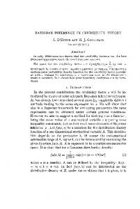
A simulated sample P consists in the distances xi and associated vectors N (z1i , z2i , z3i ) for a total n = i=1 (z1i +z2i +z3i ) detected subjects. The full sampling procedure is replicated 20 times, each identified as transect tr , where r = 1, 2, ..., 20. The observed perpendicular distances and the total number of detected subjects are summarized and displayed in Figura 1. t1
t2
t3
t4
t5
n= 86
n= 88
n= 94
n= 90
n= 90
t6
t7
t8
t9
t10
n= 91
n= 92
n= 86
n= 86
n= 81
t11
t12
t13
t14
t15
n= 81
n= 89
n= 85
n= 84
n= 83
t16
t17
t18
t19
t20
n= 92
n= 94
n= 93
n= 87
n= 91
Figure 1 - Histogram of individual distances and total sample size n for 20 replicated samples extracted from the simulated population. All the frequencies (y-coordinates) are on the same scale and distances (x-coordinates) are on the interval [0, 1].
The second data set is adapted from Quang and Becker (1997) and consists of a mixed population with two species of loons (Gavia pacifica and Gavia immer ) inhabiting the Yukon Flats National Park, Alaska. Since double count distance data were reported only in interval classes (Table 1), we simulated within each class, the individual distances with uniform distributions. Table 1 - Loon detection data reproduced from Quang and Becker (1997), Table 01 Distance class Front passenger only Rear passenger only Both passengers
5-30 3 4 0
30-60 1 3 1
60-90 2 0 2
Rev. Bras. Biom., São Paulo, v.34, n.1, p.84-106, 2016
90-120 3 3 10
120-150 3 5 6
150-190 5 1 6
190-250 5 2 2
89
2.3
Fitted model
Models used for inference are distinct regarding data type and link function. In some models, data are only perpendicular distances to the line transect (LT); in others, double observer mark-recapture data are also included (DOLT). The link functions are logit or probit. From now on we will just use model numbers in Table 2 when refering to them. From now on we will use the shorthand ’DOLT-logit’ when refering to the model fitted to double-observer distance data fitted with logit link; applying the obvious changes when refering to all other situations. In the case of LT models M1 and M2 we use the total number n of subjects detected by at least one observer and simply ignore capture-recapture information. This allows for the evaluation of changes in precision of abundance estimates obtained for the same sample size and distance data but including double observer data as well (M3 and M4).
Table 2 - List of models fitted to distance data only (LT ) and complemented by double observer mark-recapture data (DOLT ). The logit link is used in odd-numbered and the probit link in even-numbered models. The term single refers to models with a single detection function while obs refers to models with observer-specific detection functions. The term quad indicates the inclusion of a quadratic term (pji = gj (xi ))
M1 M2 M3 M4 M5 M6 M7 M8 M9 M10
Model h i pi log (1−p = β0 + β1 · x i i) −1 Φ h(pi ) = iβ0 + β1 · xi
Description single LT − logit single LT − probit
p
single DOLT − logit single DOLT − probit
p
double DOLT − logit double DOLT − probit
p
single quad DOLT − logit single quad DOLT − probit
p
double quad DOLT − logit double quad DOLT − probit
ji log (1−p = β0 + β1 · x i ji ) −1 Φ h(pji ) =iβ0 + β1 · xi
ji = βj0 + βj1 · xi log (1−p ji ) −1 Φ h(pji ) =iβj0 + βj1 · xi
ji log (1−p = β0 + β1 · xi + β2 · x2i ji ) −1 Φ h(pji ) =iβ0 + β1 · xi + β2 · x2i
ji log (1−p = βj0 + βj1 · xi + βj2 · x2i ji ) Φ−1 (pji ) = βj0 + βj1 · xi + βj2 · x2i
To fit the loon data, we further include a quadratic term of x to allow for the possibility of a maximum detection probability at some distance off the transect line (x > 0). To select the most parsimonious model we use the deviance information criterion (DIC), with smaller DIC meaning a better fit (SPIEGELHALTER et al., 2002). To facilitate later reference just by model number, all fitted models are listed in Table 2. 90
Rev. Bras. Biom., São Paulo, v.34, n.1, p.84-106, 2016
2.4
Bayesian inference - simulated data
Models 1 to 6 (Table 2) are fitted to each of the 20 replicated transects. We define vague marginal priors for all parameters: ψ ∼ U (0, 1); βj0 ∼ N (0, 1E5) and βj1 ∼ N (0, 1E5) to j = 1, 2. Posterior distributions are obtained by Markov Chain Monte Carlo (mcmc) simulations (MARTIN and QUINN, 2006; McCARTHY, 2007) with the libraries R2jags (SU and YAJIMA, 2015) and rjags (PLUMMER, 2013), which run JAGS (PLUMMER, 2003; PLUMMER, 2012) from within R (version 3.1.1) (R CORE TEAM, 2014). We evaluate convergence with the diagnostic tools Rhat and n.eff provided by R2jags, in combination with the standard diagnostics provided in the ’coda’ package (PLUMMER, 2010; PLUMMER, 2013). After some preliminary testing we have fixed the fitting procedure that achieved satisfactory convergence diagnostics, running three chains with a burn-in of 10.000 steps and a thinning of 40, generating a posterior sample of size 3000. To assess inferential efficiency in estimating population size N and detection probability at maximum detection gj (0) we use the relative bias (rb) defined as the difference between the posterior mean and the true value divided by the true value. As a summary over the twenty replicates we further calculate the average rb and also the root mean squared error (rmse) among posterior means; where rmse is defined as the variance of the posterior mean plus the squared difference between the average posterior mean and the true parameter. 2.5
Bayesian inference - loon data
Models 3 to 10 (Table 2) are fitted to the loon data with vague prior distributions for all model parameter: ψ ∼ U (0, 1); βj0 ∼ N (0, 1E5), βj1 ∼ N (0, 1E5) e βj2 ∼ N (0, 1E5). The posterior distributions are obtained as previously, with three chains, a burn-in of 10.000 steps and a thinning of 40, generating a posterior sample of size 3000. Preliminary testing indicated good convergence diagnostics when running mcmc with these options. Models with an additional quadratic term β2 (models 7 and 8) or the observerspecific extension βj2 (models 9 and 10) have the maximum detection probability at some positive perpendicular distance x0 > 0. For some fixed values β1 and β2 this distance is:
x0
= −
β1 2β2
Therefore, in a quadratic model, g(x0 ) replaces g(0) as the distance with maximum detection probability. Within the Bayesian framework, it is easy to obtain a posterior distribution for this probability, since it is a known function of the uncertain parameters β0 , β1 and β2 (or their j-indexed equivalents) for which joint posterior distribution is readily available. For the inverse-logit and inverse-probit link functions, these maximum detection probabilities are, respectively Rev. Bras. Biom., São Paulo, v.34, n.1, p.84-106, 2016
91
g(x0 )
=
g(x0 )
=
2 β1
(1 + e−(β0 − 4·β2 ) )−1 β2 Φ(β0 − 1 ) 4 · β2
For later reference, we mention that these maximum detection probabilities gj (x0 ) are equivalent to the parameters cj for observer j = 1, 2 in Quang and Becker (1997) defined in another very different model formulation. 2.6
Goodness-of-fit - loon data
The rational to evaluate the quality of model fit is to check whether, with a proposed model and the resulting parameter estimates, we are able to generate predictive distributions consistent with the observed sample data (GELMAN and HILL, 2007, p.513). That is, to compare the observed total number of detections by the front passenger only (n1o = 22), by the rear passenger only (n2o = 18) and by both passengers (nbo = 27), with the three-dimensional predictive distribution induced by the posterior distribution. Based on the given perpendicular distances xi (i = 1, ..., M ) in the augmented population of size M and given the posterior sample of size 3000 for the parameter vector θ(s) (s = 1, ..., 3000), which for the most general models (M9 and M10) is θ(s) = (ψ(s) , βj0(s) , βj1(s) , βj2(s) ) (j = 1, 2) we repeat the steps describe next for each s. Generate M random quantities wi(s) from the Bernoulli distribution with parameter ψ(s) . For each of the M subjects calculate the probability vector µi(s) = (µ1i(s) , µ2i(s) , µ3i(s) , µ4i(s) ) and simulate Zi(s) = (z1i(s) , z2i(s) , z3i(s) , z4i(s) ) from a multinomial distribution of size one and parameter µi(s) . Obtain the sums PM nr(s) = i=1 zri(s) for r = 1, 2, 3 which are the predicted numbers of subjects detected by observer one only (n1(s) ), observer two only (n2(s) ) and by both (n3(s) ). Hence, the predicted total sample size is n(s) = n1(s) + n2(s) + n3(s) . The procedure outlined in the previous paragraph, is repeated for all 3000 simulated posterior parameter vectors θ(s) to generate a predictive distributions to be confronted with observed mark-recapture data. A model with adequate fit is expected to display predicitive distributions in line with actual observations. Finally, two further model checks are used: (i) the empirical cumulative distribution function (ecdf) of observed distances is compared to ecdf-s build from predicted observed distances simulated for posterior parameter vectors θ(s) ; (ii) the observed sample size is compared to sample sizes of the posterior predicted samples,
3 3.1
Results Simulated data
All models were fitted with the logit and the probit links. However, based on DIC no link provides a uniformly superior fit. Therefore, we focus the description 92
Rev. Bras. Biom., São Paulo, v.34, n.1, p.84-106, 2016
below only on the logit link, but retain in Tables and Figures the results for both. Abundance estimation with distance data only (M1) has an average posterior standard deviation of 68, which reduces to an average of 31 when double observer data are included and a single detection function is assumed (M3) and reduces still further to 21 when observer-specific detection functions are assumed (M5)(Table 3a). However, using the posterior means of the 20 replicas we observe (rb) that models M1 and M3 are positively biased by 9% of the true value while model M5 is biased negatively by about 12% (Table 3a and 3b). A compromise between bias and precision is best described by the root mean square error (rmse) calculated over the replicated posterior means (Table 4). Based on the smallest rmse (33.76) model M5 is the best among these three models. Finally, regarding the coverage provided by the posterior 95% credibility intervals (CrI95), the true parameter N was covered by 16 out of 20 replicas for both DOLT models M3 and M5 (Figura 2). This coverage is below the 19 out of 20 as announced by the credibility interval.
t2l3
t2l3
M1
M3
M5
t1l3
t1l3
t1l3
M2
M4
M6
0
100 200 300 400
0
100 200 300 400
t2l3
Abundance estimate to modelos front M1 to M6
Figure 2 - Box-plot-type posterior distribution summaries of abundance (N ) for models M1 to M6. CrI50 (boxes), CrI95 (whiskers), median (inbox horizontal line), true parameter (horizontal line). Model comparisons with DIC consistently identified the model with observerspecific detection function M5 as better (i.e. lower DIC) than the model that assumes a single detection curve M3 (Table 3a and 3b). This consistency also holds for models with probit link (i.e., M6 is better than M4).
Rev. Bras. Biom., São Paulo, v.34, n.1, p.84-106, 2016
93
94
Rev. Bras. Biom., São Paulo, v.34, n.1, p.84-106, 2016
t1 t2 t3 t4 t5 t6 t7 t8 t9 t10 t11 t12 t13 t14 t15 t16 t17 t18 t19 t20 mean
(b)
t1 t2 t3 t4 t5 t6 t7 t8 t9 t10 t11 t12 t13 t14 t15 t16 t17 t18 t19 t20 mean
(a)
M3 g(0) 0.62 0.60 0.66 0.46 0.64 0.73 0.76 0.56 0.71 0.59 0.67 0.78 0.70 0.80 0.73 0.77 0.69 0.67 0.75 0.74 0.68
M1 N 180 255 172 153 243 255 210 253 175 242 168 260 273 267 217 201 195 228 198 197 217
sd 0.08 0.07 0.07 0.09 0.07 0.06 0.06 0.08 0.06 0.07 0.07 0.06 0.06 0.05 0.07 0.06 0.08 0.07 0.06 0.06 0.07
sd 74 71 45 53 74 73 68 74 41 86 70 65 70 71 82 61 67 74 76 61 68 M4 g(0) 0.59 0.57 0.65 0.44 0.62 0.53 0.75 0.54 0.70 0.57 0.65 0.74 0.62 0.79 0.72 0.75 0.67 0.65 0.73 0.73 0.65
DIC 4226 2696 2376 3480 3314 3051 3520 2813 1719 3820 3895 2220 2178 2242 4014 2981 3781 4000 4148 3230 3185
rb -0.046 -0.071 0.019 -0.298 -0.021 0.127 0.163 -0.144 0.090 -0.088 0.030 0.192 0.081 0.233 0.124 0.182 0.057 0.031 0.153 0.136 0.047
rb -0.10 0.28 -0.14 -0.23 0.21 0.27 0.05 0.27 -0.13 0.21 -0.16 0.30 0.36 0.34 0.09 0.00 -0.02 0.14 -0.01 -0.01 0.09
sd 81 67 45 72 78 72 70 80 40 88 84 77 85 74 67 36 67 79 75 77 71
sd 0.08 0.07 0.07 0.08 0.08 0.48 0.06 0.40 0.06 0.07 0.07 0.06 0.38 0.06 0.07 0.06 0.08 0.07 0.06 0.06 0.12
M2 N 214 258 165 165 254 261 238 234 160 183 188 250 243 236 149 138 170 220 193 203 206
rb -0.095 -0.116 -0.002 -0.326 -0.046 -0.182 0.147 -0.177 0.078 -0.123 0.003 0.144 -0.046 0.216 0.109 0.159 0.031 0.004 0.123 0.118 0.001
rb 0.07 0.29 -0.17 -0.17 0.27 0.31 0.19 0.17 -0.20 -0.09 -0.06 0.25 0.22 0.18 -0.26 -0.31 -0.15 0.10 -0.04 0.02 0.03 M5 g1(0) 0.88 0.84 0.83 0.66 0.74 0.78 0.91 0.84 0.77 0.77 0.85 0.92 0.78 0.96 0.90 0.93 0.83 0.82 0.89 0.88 0.84
DIC 4623 2454 2550 5477 3384 2831 3259 3745 2030 6060 4854 3453 3935 3026 5007 2220 5202 4838 4646 4893 3924
sd 0.06 0.06 0.07 0.11 0.09 0.07 0.05 0.08 0.07 0.08 0.06 0.04 0.07 0.03 0.05 0.03 0.08 0.07 0.05 0.05 0.06
M3 N 220 296 209 279 208 170 178 219 213 260 231 259 273 157 175 198 166 221 204 205 217 DIC 821 1113 1013 1194 992 772 771 1151 888 1150 1005 815 990 608 784 782 720 941 798 877 909
g2(0) 0.42 0.45 0.50 0.30 0.51 0.68 0.60 0.38 0.63 0.41 0.51 0.62 0.63 0.63 0.59 0.60 0.57 0.54 0.63 0.59 0.54
rb 0.10 0.48 0.05 0.40 0.04 -0.15 -0.11 0.09 0.06 0.30 0.16 0.30 0.36 -0.22 -0.13 -0.01 -0.17 0.11 0.02 0.02 0.09
rb 0.098 0.046 0.038 -0.172 -0.079 -0.027 0.133 0.046 -0.032 -0.041 0.064 0.151 -0.030 0.196 0.121 0.165 0.039 0.020 0.108 0.102 0.047
sd 38 39 28 51 31 22 20 38 27 38 31 32 36 20 22 23 25 31 26 25 31
sd 0.08 0.08 0.09 0.08 0.09 0.08 0.08 0.08 0.08 0.08 0.08 0.08 0.08 0.08 0.09 0.08 0.10 0.09 0.08 0.08 0.08
M4 N 216 293 207 278 206 289 175 288 209 257 227 256 316 155 176 195 164 219 200 201 226
rb -0.160 -0.105 -0.004 -0.397 0.029 0.361 0.209 -0.238 0.257 -0.180 0.022 0.243 0.254 0.253 0.181 0.200 0.137 0.071 0.259 0.189 0.079
sd 38 40 28 50 31 69 20 63 27 38 30 32 48 19 22 23 26 31 25 23 34 M6 g1(0) 0.88 0.84 0.81 0.65 0.73 0.78 0.91 0.82 0.77 0.77 0.84 0.94 0.76 0.96 0.90 0.94 0.82 0.79 0.89 0.88 0.83
rb 0.08 0.47 0.04 0.39 0.03 0.44 -0.12 0.44 0.05 0.29 0.14 0.28 0.58 -0.23 -0.12 -0.02 -0.18 0.10 0.00 0.00 0.13
sd 0.07 0.07 0.08 0.11 0.09 0.07 0.05 0.09 0.07 0.08 0.06 0.04 0.07 0.03 0.06 0.04 0.09 0.08 0.05 0.05 0.07
DIC 839 1180 1023 1156 984 738 787 996 878 1192 1001 827 922 614 804 799 766 973 784 838 905
sd 25 24 17 44 23 18 15 23 19 23 19 16 24 13 18 17 19 22 17 18 21
rb 0.097 0.051 0.010 -0.192 -0.087 -0.031 0.133 0.028 -0.032 -0.042 0.054 0.170 -0.047 0.202 0.124 0.181 0.024 -0.008 0.113 0.100 0.042
M5 N 177 216 167 224 173 154 158 170 174 186 181 185 227 133 164 177 140 184 166 175 176
g2(0) 0.41 0.44 0.47 0.32 0.50 0.67 0.59 0.37 0.62 0.41 0.50 0.59 0.61 0.61 0.59 0.59 0.55 0.51 0.63 0.60 0.53
rb -0.12 0.08 -0.17 0.12 -0.13 -0.23 -0.21 -0.15 -0.13 -0.07 -0.10 -0.08 0.13 -0.33 -0.18 -0.12 -0.30 -0.08 -0.17 -0.12 -0.12
sd 0.09 0.08 0.09 0.08 0.09 0.08 0.08 0.08 0.08 0.08 0.08 0.08 0.08 0.08 0.09 0.08 0.10 0.09 0.08 0.08 0.08
DIC 665 1005 837 1303 927 749 708 908 816 1045 863 623 882 492 708 658 673 857 670 771 808
M6 N 161 202 159 216 168 149 146 164 176 198 194 178 200 121 157 164 131 173 173 165 170
rb -0.175 -0.123 -0.067 -0.365 0.008 0.340 0.178 -0.255 0.248 -0.180 0.008 0.180 0.230 0.225 0.179 0.175 0.107 0.020 0.259 0.204 0.060
Table 3 - (a) Posterior means of abundance, (N); standard deviation, (sd); relative bias, (rb) and DIC. (b) Posterior means of g(0); standard deviation (sd); relative bias (rb) for M1 to M4; and g1 (0) and g2 (0) for M5 and M6 sd 22 22 18 39 21 16 14 25 19 25 20 16 20 11 16 16 17 20 17 15 19
rb -0.20 0.01 -0.20 0.08 -0.16 -0.25 -0.27 -0.18 -0.12 -0.01 -0.03 -0.11 -0.00 -0.40 -0.21 -0.18 -0.34 -0.13 -0.13 -0.18 -0.15
DIC 656 953 948 1184 892 704 679 1021 800 1063 825 635 862 483 650 665 653 839 630 709 793
In all DOLT models the estimates of g(0) have a good performance. For the observer-specific model M5, these estimates have a positive bias of 5% and 8% for observers one and two, respectively (Table 3a and 3b). Hence, they are less biased than estimates of abundance described previously. Model M3, that assumes a single detection function is also quite able to estimate the average between the true values (0.8 and 0.5) for both observers, which is g(0) = 0.65 (Table 3a and 3b). Regarding coverage of the 95% credibility intervals, 17 and 18 out of 20 are the success rates for observers one and two in model M5 (Figura 3).
g1(0)
g2(0)
g1(0)
g2(0)
0.6 0.4 0.6 0.4 0.0
0.2
Model M6
0.8
1.0
0.0
0.2
Model M5
0.8
1.0
gzero estimate
Figure 3 - Box-plot-type posterior distribution summaries of detection probability at distance zero for observer 1 (g1 (0)) and observer 2 (g2 (0)) for simulated data fitted to models M5 and M6. CrI50 (boxes), CrI95 (whiskers), median (inbox horizontal line), true parameter (dotted horizontal line).
3.2
Case study
All linear and quadratic DOLT models listed in Table 2 were fitted to the loon data; summaries are in Table 5. The models with smallest DIC are M8 and M10 which include a quadratic term for observed distances and uses the probit link. However, both models are indistinguishable regarding predictive performance, since DICs differ only by one unit. In fact, differences in abundance estimates N are negligible since they have posterior mean 156 (CrI95: 128 to 189) and 154 (CrI95: 125 to 185) for models M8 and M10, respectively. Nevertheless, these estimates exceed in about 35% the estimated 99 individuals obtained by Quang and Becker (QB). For further comparisons with results by QB, we focus on model M10 which Rev. Bras. Biom., São Paulo, v.34, n.1, p.84-106, 2016
95
retains observer-specific detection functions as they did. In model M10 the observer-specific detection probabilities at distance zero (g1 (0), g2 (0)) and the detection probabilities at the distances of maximum detection probabilities (g1 (x10 ), g2 (x20 )) are higher than the corresponding estimates reported by QB (Table 4; 5; Figura 4c and 4d). However, while posterior standard deviations in the former estimates are similar to the asymptotic standard errors (ASE) presented by QB, our values are much smaller for the latter where posterior standard deviation are close to 0.05 while the ASEs are above 0.25 (Table 4). Table 4 - Summaries over 20 replicated simulations of the posterior mean for abundance N : average (mean); standard deviation among posterior means (sdpm); root mean square error (rmse) and average DIC among replicates (DICm ) mean sdpm rmse DICm
M1 217.264 37.134 40.951 3185
M2 206.169 39.866 40.340 3924
M3 217.003 39.544 43.044 909
M4 226.419 47.167 54.062 905
M5 176.464 24.197 33.755 808
M6 169.809 23.927 38.523 793
Table 5 - Posterior mean and sd for abundance (N ); detection probability at distance zero for single detection function or for observer 1, (g1 (0)) and for observer 2, (g2 (0)); maximum detection probability at distance x0 for single detection function or for observer 1, (g1 (x0 )) and for observer 2, (g2 (x0 )). Last line (QB) reproduces maximum likelihood estimates and asymptotic standard error from Quang and Becker (1997) M3 M4 M5 M6 M7 M8 M9 M10 QB
N 84 85 82 83 144 156 141 154 99
sd 7.38 7.72 6.84 6.85 14.11 15.58 14.19 15.12 6.34
g1(0) 0.440 0.442 0.396 0.338 0.224 0.124 0.202 0.095 0.110
sd 0.124 0.122 0.091 0.136 0.056 0.056 0.068 0.058 0.080
g2(0) 0.531 0.541 0.302 0.193 0.162
sd 0.096 0.148 0.103 0.094 0.089
g1(x0) 0.852 0.902 0.876 0.879 0.754
sd 0.040 0.041 0.052 0.054 0.256
g2(x0) 0.932 0.924 0.732
sd 0.052 0.056 0.283
DIC 477 498 453 454 278 251 287 252 -
Goodness-of-fit diagnostics suggest that model M10 is less capable of adequately predicting the observed number of mark-recapture data than the simpler model M6 (Figura 5 and 6). The graphic displays suggest that M10 predicts larger sample sizes of detected loon than the 67 individuals that were actually observed. Only with regard to the predicted distribution of distances (Figura 6) M10 seems to be slightly superior. This results are surprising because M10 has a much smaller DIC than M6 and therefore one would expect to observe features in support of a better fit.
96
Rev. Bras. Biom., São Paulo, v.34, n.1, p.84-106, 2016
Modified Quang & Becker, 1996 QB´Data
N
16
12
7 5
100 150 200 250
0
50
100
n=67
N=98.99
g1(x0)
g2(x0)
150
200
Frequency
50
9
4
Frequency
0
Frequency
Density
14
0.5
0.6
0.7
0.8
0.9
1.0
0.5
c1=0.7544
0.6
0.7
0.8
0.9
1.0
c2=0.7323
Figure 4 - Top left: histogram of observed data by QB; Top right: posterior distribution for abundance N and the corresponding estimate with confidence range by QB [vertical lines]; Bottom left: posterior distribution of highest detection probability for observer 1 [g1 (x0)] and the estimate of this parameter (c1 ) by QB [vertical line]; Bottom right: posterior distribution of highest detection probability for observer 2 [g2 (x0)] and the estimate of this parameter (c2 ) by QB [vertical line]. All posterior distributions refer to model M10.
Rev. Bras. Biom., São Paulo, v.34, n.1, p.84-106, 2016
97
80
M6
80
M10
n2
40
● ● ●● ●● ●●●● ●●● ● ●● ● ●● ●●●●●● ●●● ● ● ● ●●● ● ● ● ● ●●● ●● ●● ●● ● ●● ●●●●●● ●● ●●● ●● ● ●● ● ●● ●● ●● ● ● ● ● ● ●● ● ●● ●● ● ●●●●● ●● ● ● ●● ●● ●● ●● ●●● ● ● ●● ● ● ● ●● ●●●●● ●● ● ●● ● ● ●● ● ●● ●● ●● ●● ● ●● ●● ●● ● ●● ● ●● ●● ●●● ● ●● ●● ● ● ● ●● ●● ●● ● ● ● ●●●● ●● ● ●● ● ● ●● ● ● ● ● ●● ● ● ● ● ● ● ● ● ● ● ●● ●●● ●●● ● ●● ● ● ●● ●● ●● ●● ● ● ● ●● ● ●● ● ●● ●● ●● ● ●● ● ●● ● ● ●● ●● ● ● ● ● ●● ● ● ● ●● ● ● ● ● ● ● ● ●● ● ●● ●● ●● ● ●● ●● ● ● ●● ● ●● ●● ●● ● ●● ● ● ● ●● ●● ●●● ●● ●● ●● ●● ● ●● ● ● ● ●● ●● ●● ● ● ● ●● ●● ● ●● ●● ● ●●●●● ● ● ● ●● ● ● ● ● ● ● ● ● ● ● ● ● ● ● ●● ●● ●● ●● ●● ● ●● ●● ●● ● ● ● ● ● ● ● ● ● ● ● ●● ● ● ● ●● ●● ●●● ● ● ●● ● ●● ● ●●●●● ●● ●
0
40 0
n2
●
●●●● ●●●● ● ●●● ● ●●●●●●●● ●●● ● ● ●●● ● ●●●●● ●● ● ●● ●● ● ●●● ● ● ●● ● ● ●● ● ● ● ●● ● ●●● ● ● ●● ●● ●● ●● ●● ●●● ●● ● ●●●● ● ● ●● ●● ●● ● ● ● ●● ●●●●●●● ● ● ● ● ● ●● ● ●● ●●●● ●● ●● ● ●● ● ●● ●● ●● ●● ●● ●● ●● ● ● ●● ●● ●● ●● ●● ●● ●● ● ●● ● ●●● ● ● ●● ●● ● ●● ● ● ●● ● ● ●● ●● ●● ●●● ●●●●● ●● ●●●●● ●● ● ●● ● ● ●● ●● ● ● ● ●● ●● ●● ● ●● ●● ●● ● ● ● ● ● ● ●● ● ● ● ● ● ●●●● ● ●● ● ●● ●● ●● ●● ●●● ●●● ●● ●● ●● ●● ● ● ●● ●● ●● ●● ● ● ●● ●● ●● ●● ●● ●● ●● ●● ● ● ●● ●● ●● ● ● ● ● ●● ● ● ●● ● ● ●● ●● ● ● ● ●● ●● ● ● ● ● ● ● ●● ● ● ● ● ● ● ●● ●● ● ● ● ●● ●● ●● ●●●● ●● ●● ●● ● ● ●● ● ●● ●● ● ●● ●● ●● ●● ● ●● ● ● ● ● ● ● ● ● ● ● ● ● ● ● ● ● ●● ● ● ● ● ● ●● ●● ●● ●● ● ●● ●● ●● ●● ●●● ●●● ● ● ● ● ● ●● ●● ●● ● ● ●● ●● ●● ●● ● ● ● ● ● ● ●● ●● ● ● ●● ●● ● ●● ●● ● ● ●● ●● ● ● ● ● ● ● ● ● ● ● ●● ● ● ●● ●● ●● ●● ●● ●● ●● ●● ●● ●● ●●●●●●●● ● ●● ●● ●● ●● ●● ● ●● ● ● ● ●●● ●● ●● ●● ● ●● ● ●● ● ●●● ● ●● ● ● ● ●● ●●● ●●●● ●● ●● ● ●●● ● ● ● ● ● ● ●● ● ●●●● ●●●●● ● ●●●● ● ●●●●● ●●●●●
0
20
40
60
80
100
0
20
40
n1
20
40
80
100
0
20
40
80
100
60
80
100
80 0
n3
● ● ●● ●● ● ●●● ●● ●●● ●● ● ●● ● ● ●● ● ●● ●● ●●● ●● ●● ● ●● ● ●● ●● ●● ●● ●● ●● ●● ● ● ● ●● ●● ●● ●● ●●●● ●● ● ● ● ●● ● ● ●● ●● ● ●● ● ● ● ● ● ●● ●● ●●●●● ●● ● ●● ●● ●● ●● ●● ●● ● ●● ● ●● ● ●● ●● ● ● ●● ●● ● ●● ● ●● ●●●● ● ● ● ● ● ● ● ● ● ● ●●●●● ● ● ● ● ● ● ● ●● ● ● ● ● ● ● ●● ● ● ●● ● ● ●● ●● ●● ●● ● ●● ●● ●● ● ● ●● ● ● ● ●● ● ●● ●● ● ● ● ●● ● ● ● ●● ● ● ●● ●● ● ● ● ● ● ● ● ● ● ● ● ● ● ● ●● ● ●● ● ●● ●●●●●●●● ●● ●● ● ● ●●● ● ●● ●● ●● ●● ●● ● ● ● ●● ●● ● ● ●● ● ●● ●● ● ● ●● ●● ● ●● ●● ●● ●● ● ●● ●● ● ● ● ● ● ● ● ● ● ● ● ● ● ● ● ● ●● ●● ●●●●● ●● ● ●● ● ● ●●● ● ● ● ● ● ● ● ●● ● ●● ●● ● ●● ●● ● ●● ● ●● ● ● ● ●● ●● ●● ●● ● ● ●● ● ●● ●● ● ●● ● ●● ●●● ● ●● ●● ● ● ● ●●● ●● ●● ●● ●● ●● ●●● ●● ●● ● ● ●● ●● ●● ●●●● ●●● ● ● ●● ●● ●● ●● ●●● ●● ●● ●●● ● ●● ●● ●● ● ● ● ● ● ●● ● ●●●● ●● ●● ●● ● ●● ●●●● ●● ● ●● ● ●
40
80
n3
40 0
40
60
n2
●●● ●● ● ● ●●●●●● ● ● ●● ● ●●● ●●● ● ●● ●●●● ● ●● ●● ●●●● ●●●● ●● ●● ●● ● ● ●● ● ●● ●●● ●● ●●● ●●●● ● ● ●● ●● ●●● ●●● ●● ●●● ●●● ●● ● ●●● ● ●● ●● ● ●● ●● ●● ●●● ● ●● ●● ●●● ● ● ●● ●● ●●● ● ● ● ● ●● ● ●●● ● ●● ● ●● ●● ● ● ● ● ● ● ●●● ● ●● ● ● ●● ●● ●● ● ●● ● ●●●● ●● ● ● ● ●● ● ● ● ● ● ● ● ●● ● ●● ●●● ●● ● ● ●● ●● ● ●● ●● ●● ●● ● ● ● ● ●●● ●●● ● ●● ● ● ● ●● ● ●● ●● ● ● ●● ●● ●● ●● ● ● ●● ● ● ●● ● ● ●● ● ● ● ● ● ● ● ● ● ●●●● ●● ● ● ● ● ● ●● ● ● ● ● ● ● ●● ●● ●● ●● ●● ●● ●● ●● ● ●●● ●● ●● ●● ●● ● ●● ●● ●● ● ●● ● ●● ● ●●● ●● ●● ● ●● ●● ● ● ●● ● ● ● ●● ●● ● ●●● ● ●●●●● ●● ● ●● ● ● ● ● ● ●● ●● ● ●●● ● ● ● ● ● ●● ● ●● ●● ●● ● ●● ●● ●● ●● ●● ● ●● ● ●● ● ●● ●● ●● ●● ● ●● ●● ●● ●● ● ● ●● ● ●● ●● ● ● ● ●● ● ● ● ● ● ●●● ● ● ●●● ● ● ●● ● ● ●●● ●● ●● ●● ● ●● ●● ●● ●● ●● ●● ●● ●● ● ● ● ●● ●● ●● ● ●● ●● ●● ●● ● ● ● ● ● ● ● ● ● ● ● ● ● ● ● ● ●● ● ●● ●●●● ●● ●● ●● ●● ●●● ●● ●● ●● ●● ●● ●●● ● ●● ●● ●●● ●● ●● ●● ●●●●●● ●● ●● ●● ● ●● ●● ● ●● ●● ● ● ● ●● ● ● ● ● ● ● ●● ● ● ●●●● ●●● ● ●● ● ● ● ● ●● ● ● ● ● ●● ●● ● ●● ●● ●● ● ●● ●● ● ● ●● ●● ●●●● ●● ●● ●●● ● ● ●● ● ●● ●● ●● ●● ●● ●● ●●●●● ● ● ● ● ● ● ●● ● ●●●● ●● ● ●●● ●● ●● ●● ● ●●● ●● ●● ● ●●● ● ● ● ● ●●●●● ● ● ● ● ● ● ●●● ● ● ● ● ● ● ● ● ● ● ●●●● ●●●●● ● ●●●● ●●● ●● ● ● ● ●●●● ●
20
100
80 40
n3
60
n2
0
80
● ●● ● ● ● ● ● ● ● ● ●●● ● ●● ●●● ●●●● ● ●● ●● ●●●● ● ●●●● ●● ●● ● ● ●●● ●● ●● ● ●● ●● ● ●● ●●● ●● ●●●●●● ●●●●● ●● ●● ●● ● ● ● ● ● ●● ●● ●● ● ● ●● ● ●● ●● ● ●● ● ●● ●● ● ● ● ● ●● ● ●● ● ● ● ● ● ● ●● ●●●● ● ●● ● ● ●● ● ● ●● ● ●● ●● ●● ● ●● ● ● ●● ● ● ● ● ●● ●● ●● ● ●● ● ●● ●● ●● ●● ● ●● ●● ● ●● ● ● ●● ● ● ● ● ● ● ● ● ●● ● ● ● ● ●● ● ●● ●● ●● ●●●●●●●●● ●● ●● ●● ●● ●● ●● ● ● ●● ●● ●● ● ●● ● ●● ●● ● ●● ●● ●● ● ● ●● ●● ● ● ● ● ●● ●● ● ●● ● ●● ●● ● ●● ● ●● ● ●● ●● ●● ●● ●● ●● ●● ●● ●● ● ●● ●● ●● ●● ● ●● ●● ● ●●● ●● ●● ●● ● ●● ● ● ●● ●● ●● ●● ● ●●● ● ● ●● ● ●●● ●● ● ●● ●●● ●● ●● ●● ●● ●● ●● ●● ●● ●●●● ●● ●● ●● ●● ●● ●● ● ●●● ●●●● ●● ● ●● ● ● ● ● ● ● ● ● ● ● ●●●● ● ● ● ● ●●●●●●●● ●●● ●● ●●
0
n3
0
40
80
● ● ● ● ●●● ●● ● ●●●● ●● ●● ●● ●●● ● ●●● ●● ●● ●●● ● ●● ●●● ●●● ●● ● ●●● ●● ● ● ● ●●● ● ● ● ● ●● ● ●● ●● ●● ●● ●●● ●● ●●●●● ● ● ●● ● ● ● ●● ●● ●●● ● ● ● ● ● ●● ●● ●● ●● ● ●● ●● ●● ●● ● ● ●● ●● ●● ●●● ● ●● ●● ● ● ●● ●● ●● ●● ● ● ● ●● ● ●●●● ●●● ● ● ● ● ●● ● ●● ●● ● ● ● ● ● ● ●● ● ● ●● ● ● ● ●● ●● ●● ●● ● ● ●● ● ●●●● ●● ● ●● ● ● ● ● ● ● ● ● ●● ● ● ●● ●●● ● ● ● ● ● ●● ● ● ● ● ● ● ● ●● ●● ●● ● ●● ●● ●● ●● ● ●● ●●● ●●●● ● ●● ●● ●● ● ● ● ●● ●● ●● ● ● ●● ● ●● ● ● ● ● ● ●● ●● ●● ●●● ● ● ● ● ● ● ● ●● ●●● ● ●● ● ● ●● ● ●● ●● ●● ● ●● ●● ●● ●● ● ●● ●● ●● ●● ●● ● ●●● ●● ●● ●● ●● ●●●●● ●● ● ● ●● ● ● ● ● ● ● ●● ● ● ●● ●● ●● ● ● ● ● ●● ● ●● ● ●● ● ●● ●●● ● ● ● ●● ● ●● ●● ●● ●● ●● ● ●● ●● ●● ● ● ● ●● ●● ●● ●● ● ●● ●●● ●● ●● ●● ●● ●● ●● ●● ●● ●● ● ● ● ●● ●● ●●● ● ● ●● ● ● ●● ● ●● ● ● ●● ● ● ● ● ● ● ● ● ● ● ● ● ● ● ●● ●● ●● ●● ●● ●● ●● ●●●●●●● ●● ●● ●● ●● ●● ●● ●● ● ●● ●● ●● ●● ●● ●● ●● ● ●● ●● ●● ●● ● ●● ● ●● ● ● ● ●● ●●●● ●●● ● ●● ●● ●● ● ●● ● ● ● ● ● ● ● ● ● ● ●● ● ● ● ● ● ●● ●● ● ● ● ● ●● ● ●● ●●●●● ● ●● ●● ● ●● ●● ●● ●● ● ● ●● ●●●● ●●● ●● ●● ● ● ●● ●● ● ● ●●● ●● ● ●● ●● ●● ●● ●● ●● ●● ● ● ● ●● ● ● ●● ● ● ● ● ● ● ● ● ● ● ● ● ● ● ● ● ● ● ● ● ● ● ● ● ● ●●●●● ●●●●●●● ●●● ●● ●●● ● ●●● ●● ● ● ●
0
60
n1
60
80
100
0
20
n1
40
n1
Figure 5 - Predictive multivariate distribution under models M10 (left column) and M6 (right column) [grey dots]. n1 - number of individuals detected by observer one only; n2 - by observer two only; n3 - by both observers. The observed numbers (n1o , n2o , nbo ) are displayed with black dots.
0.0
0.4
Fn(x)
M6
● ● ● ● ● ● ● ●● ● ●● ●● ● ● ● ● ● ● ●● ● ● ● ●● ● ● ● ● ● ● ● ● ● ● ● ● ● ●● ●● ● ●● ● ● ●● ● ● ● ●● ●● ●● ● ● ● ● ● ● ● ● ● ●● ● ● ●● ● ● ● ●● ●● ● ● ● ● ● ● ● ●● ● ●● ● ● ●● ● ● ● ● ●● ● ● ● ● ● ● ● ● ● ● ● ●● ●●● ● ● ● ● ● ● ● ● ● ● ●● ● ● ● ● ● ● ● ● ● ● ● ● ● ● ● ● ●● ●● ● ● ● ● ● ●● ● ● ● ● ● ● ● ●● ● ● ● ● ●● ● ●● ● ● ●● ●● ● ● ● ● ● ● ● ● ● ● ●● ● ● ● ● ●● ● ●●● ● ●● ● ● ● ● ● ●● ● ● ●● ● ● ● ● ● ● ● ●● ● ● ● ● ● ● ● ● ● ●● ● ● ● ● ● ●● ●● ● ● ● ● ● ● ● ● ● ● ● ● ● ● ● ●● ● ● ● ● ●● ● ● ● ●●● ● ● ● ● ●● ● ● ● ●● ● ● ● ●● ●● ● ●● ● ● ● ● ● ● ● ●● ● ● ● ● ●● ● ● ● ●● ● ● ●● ●●● ●● ● ● ●● ●● ● ●● ● ● ● ● ● ● ●● ● ●● ● ●● ● ● ● ● ● ●● ●●● ● ● ●● ● ● ● ● ●● ●● ● ●● ● ● ● ● ● ● ● ● ● ● ●● ● ● ● ●● ●● ● ●● ● ● ● ● ● ● ● ●● ●● ● ● ● ● ●● ● ●● ● ● ● ●● ● ● ● ● ● ● ● ● ● ● ● ● ● ● ● ● ● ● ● ● ● ●● ● ● ● ● ●● ● ●● ●● ● ● ● ● ●● ● ●● ● ● ● ●● ● ● ●● ● ● ● ● ● ●● ● ● ● ●● ● ● ●●●● ● ● ● ● ● ● ● ● ● ● ● ● ● ● ● ● ● ●● ● ● ● ●● ● ● ● ● ●● ● ● ●● ● ● ●● ● ● ● ● ●● ● ● ● ●● ● ● ● ● ●● ●● ● ● ● ●● ●● ●● ● ● ● ● ● ● ●● ● ● ● ● ● ● ●● ● ●● ● ● ●● ● ● ● ● ● ● ● ● ● ● ● ● ● ● ● ●● ●● ● ● ●● ● ● ● ● ● ● ●● ● ● ● ● ● ● ●● ●● ● ● ● ●●● ● ● ● ● ● ● ● ● ● ● ●● ● ●● ●● ● ● ● ● ● ● ● ● ● ● ● ● ● ● ● ●● ● ● ● ● ● ● ● ● ● ● ●● ● ● ● ● ● ● ● ● ● ● ● ● ● ● ● ● ● ● ● ●● ●● ● ●● ● ● ● ● ● ● ●● ● ●● ●●● ● ●● ● ● ● ● ● ● ● ● ● ●● ● ● ● ● ● ● ●● ● ●● ● ●● ●● ● ●● ●● ● ● ● ● ● ● ● ●● ● ● ● ● ● ● ● ● ● ● ●● ●● ●● ● ● ● ● ● ● ● ● ● ● ● ● ●● ●● ● ● ●● ● ● ● ● ● ● ● ● ●● ● ●● ● ● ● ● ● ●●● ●● ● ● ● ● ● ●● ● ● ●● ● ● ●● ● ● ● ● ● ● ● ●● ● ● ● ● ● ● ●● ●● ● ● ● ● ● ● ● ●●●● ● ● ●● ● ● ● ● ● ● ●● ● ● ● ● ●● ● ● ● ●● ● ● ● ● ● ● ● ● ●● ● ● ● ● ● ●● ● ● ● ● ● ● ● ●● ● ●● ● ● ● ● ● ● ● ● ● ●● ● ● ● ●● ●● ●● ● ● ● ● ● ● ●● ● ● ● ● ● ● ●● ● ●● ● ● ● ● ● ● ● ● ● ● ● ● ● ● ● ● ● ● ●● ●● ● ● ● ● ● ● ● ●● ● ● ● ● ●● ● ● ● ● ●● ● ● ● ●● ●● ● ● ●● ● ● ● ● ●● ● ● ● ● ● ● ● ● ● ● ● ● ● ● ● ● ● ● ● ●●●● ● ● ● ● ● ●● ● ● ● ● ● ●● ● ● ● ● ● ●● ● ● ● ●●● ● ● ● ● ● ● ● ● ● ● ● ● ● ●● ● ● ● ● ●● ● ● ● ● ● ●● ● ● ●● ● ●● ●● ● ● ● ● ● ● ● ● ● ● ● ●● ● ● ● ● ●● ● ● ● ● ● ● ●● ● ● ● ● ● ● ● ●● ● ●● ● ● ● ● ● ●● ● ● ● ● ● ● ● ● ● ● ● ●● ● ● ● ● ● ●● ●● ● ● ● ● ● ● ● ● ● ● ● ● ●● ● ● ● ● ● ● ● ● ●● ● ● ● ● ● ● ● ● ● ● ● ● ● ● ● ●● ● ● ● ● ● ● ● ● ● ● ● ● ● ● ● ● ● ● ●● ● ●● ● ● ● ● ● ● ● ● ● ● ● ●● ● ● ● ●● ● ● ● ● ● ● ● ● ● ● ● ● ● ● ● ● ● ● ● ● ● ● ●● ●● ● ●●● ● ●● ●● ●● ● ● ● ● ● ● ●● ● ● ●● ●● ● ● ●● ● ● ● ●● ● ●● ● ●● ● ● ● ● ●● ●● ● ●● ● ●● ● ● ● ●●● ●●● ●● ● ● ● ● ● ● ●● ● ●● ● ●● ● ● ●● ● ● ● ● ● ●● ● ● ● ● ●● ●● ● ●● ● ●● ● ● ●● ●● ●● ● ● ● ● ● ● ● ●● ●● ● ● ● ●● ● ● ●● ● ●● ● ● ●● ●● ● ● ●● ●●● ● ● ●● ● ●● ● ●● ● ●● ● ●● ● ● ●● ● ● ● ● ●● ● ● ● ● ● ● ● ● ●● ● ● ●● ● ●● ● ●● ● ● ●● ●●● ● ● ● ●● ● ● ● ● ● ● ●● ● ●● ● ● ● ● ●● ● ● ● ●● ● ● ● ● ● ●● ●● ● ● ● ● ● ● ●● ● ● ●● ● ●● ● ● ● ● ● ●● ● ● ● ●● ● ● ● ● ● ●● ● ● ● ● ● ● ●● ● ● ● ● ● ● ● ● ● ●● ● ● ● ● ● ● ●● ●● ● ● ●●● ●● ● ● ● ● ● ●● ● ●● ●●● ● ● ● ● ● ● ● ●● ● ● ●● ● ● ● ● ● ● ●● ●●● ● ● ●●● ● ● ● ● ●● ● ● ● ● ● ● ● ● ● ● ● ●● ● ● ●● ●● ●●●● ● ●● ● ● ●● ● ● ● ● ● ●● ● ● ● ● ●● ● ● ● ● ●● ●● ● ● ● ● ● ● ● ●● ●● ●● ●● ● ●● ●● ● ● ● ● ● ● ● ● ● ● ●● ● ●● ● ● ● ● ● ● ● ● ● ● ● ●● ● ●● ● ● ● ● ● ●● ● ● ● ●● ●● ● ● ● ● ●● ● ● ●● ● ●● ● ● ● ● ●● ●● ● ● ● ● ● ● ● ●● ●● ● ● ● ● ● ●● ● ●● ●● ● ● ● ●● ● ●● ● ● ●● ● ● ● ● ●● ● ● ●● ●● ● ● ● ●● ● ● ●● ● ●● ● ● ● ● ● ● ● ● ● ● ●● ● ● ●●● ● ● ●● ● ● ● ● ● ● ● ● ●● ●● ● ●● ● ● ● ● ● ● ● ● ●● ● ● ● ● ● ● ● ● ● ● ●● ● ● ● ● ● ● ● ● ● ● ● ● ●● ● ● ●● ● ●● ● ● ● ● ● ●● ●●● ● ● ● ● ● ● ●● ● ● ● ● ● ● ● ● ● ● ● ● ● ● ● ● ● ● ● ● ● ● ● ● ● ● ● ● ● ● ● ● ● ●● ● ● ● ● ● ● ● ● ● ● ● ● ● ● ● ● ●● ●● ● ● ● ● ● ● ● ● ●● ● ●
0.0 0.2 0.4 0.6 0.8 1.0
Fn(x)
0.0 0.2 0.4 0.6 0.8 1.0
M10
0.8
● ●● ● ●● ● ●● ● ● ● ● ● ● ● ●● ●● ● ● ● ● ● ● ●● ● ● ● ●● ● ● ● ● ● ● ● ● ● ● ● ● ● ● ●● ● ● ● ● ● ● ● ● ● ● ● ● ● ● ● ●● ● ● ● ● ● ● ● ●● ● ● ● ● ● ●● ●● ● ●● ● ● ● ● ●● ● ●● ● ● ● ● ● ● ● ●●● ●● ● ● ● ● ● ●● ●● ● ● ● ● ● ● ●● ●● ● ● ● ● ● ●● ● ● ● ●● ●● ● ●● ●● ●●● ● ● ●● ● ● ● ●● ● ● ●● ● ● ● ● ●● ●● ● ● ● ● ● ●● ●● ● ● ● ●●●● ● ● ● ● ●● ● ● ● ● ● ●● ● ● ● ● ● ● ●●● ●● ● ● ● ● ● ● ●● ●● ● ● ● ●●● ●● ● ●●● ● ● ● ● ●● ●● ● ● ● ● ●● ● ●● ●● ●● ● ●● ● ●● ●●●● ● ● ● ● ● ● ●● ● ● ● ● ●●● ●● ●● ● ●● ●● ● ● ● ●● ●● ● ●● ● ● ●● ● ● ● ●●● ●● ● ● ● ●● ● ●● ● ● ● ● ●● ● ●●● ● ● ●● ●● ● ● ● ● ● ● ● ● ● ● ● ● ● ●● ● ● ● ●● ● ● ●● ● ●● ● ●● ● ● ● ● ● ● ● ● ● ●● ● ●● ● ● ●● ● ● ●● ● ●● ● ●● ● ● ●● ● ●● ● ● ● ●● ● ● ● ● ● ●● ● ● ● ●●● ● ● ● ● ● ● ● ●● ● ●● ● ● ● ● ● ● ● ●●● ● ●●● ● ●●●●● ● ●●● ● ● ● ● ● ● ● ● ● ● ● ●● ● ● ●● ● ● ● ●● ● ● ● ●●● ● ● ● ● ●● ●● ●●●● ● ● ● ● ● ● ● ●● ●● ● ● ● ●● ● ● ● ●● ● ●●● ● ● ● ● ● ● ●● ● ● ● ● ● ● ●● ●● ● ● ● ● ●● ● ● ● ● ● ● ●● ● ● ● ● ● ● ●● ● ●●● ● ● ● ● ● ● ● ● ● ● ●●● ● ● ●● ● ● ● ● ● ●●● ● ● ● ● ● ● ● ● ● ● ● ● ● ● ● ● ● ● ● ● ● ●● ● ● ●● ●● ● ● ●● ●● ● ●● ● ● ● ● ● ● ●● ●● ● ●● ● ● ●● ● ● ● ●● ● ●● ● ●● ● ●● ● ● ● ● ● ● ● ●● ● ● ● ● ● ● ● ●● ● ● ● ●●● ● ●● ● ●● ●● ● ●● ● ● ● ● ●● ●● ● ● ●●● ●● ●●● ● ● ●● ●● ● ● ●● ● ● ●● ● ● ● ●● ●● ● ● ●●●●● ●● ● ● ● ● ● ● ●● ● ●● ● ● ● ● ●●●●● ● ●●● ●● ● ● ● ● ● ● ● ●●● ●●● ●● ●● ● ● ● ● ●● ●● ● ● ● ● ● ● ●●● ● ● ● ● ● ● ● ● ●●●●●●● ● ● ● ● ● ● ● ● ● ● ● ● ● ● ● ● ● ●● ●● ● ● ● ● ●●● ●● ● ● ●● ● ● ● ●● ● ● ●● ●● ● ● ●● ● ●● ●●● ● ● ● ●● ● ● ● ● ● ● ● ●● ● ●● ●● ●●● ● ●● ● ●● ● ● ●● ● ● ● ●● ● ● ● ● ●● ●● ●● ● ●● ● ● ●● ●● ● ● ● ●●● ●● ● ●● ●● ● ● ●● ● ●● ● ●● ●● ● ● ● ● ● ● ● ●●● ●● ●● ● ●● ●● ● ● ● ● ●● ● ● ● ●● ●●● ● ●● ● ● ● ● ● ●●●● ● ● ● ●● ●● ● ●● ● ● ● ● ● ● ●● ● ● ● ● ●●● ● ●●● ●●●● ●● ● ● ● ● ● ● ● ●● ● ●● ● ●● ● ● ●● ● ●●●● ● ● ● ● ● ● ● ●●● ● ● ● ●● ● ● ● ● ●●● ● ● ● ● ● ●●●● ●● ● ●● ●● ● ● ●● ● ● ● ● ● ● ● ●● ●● ● ● ● ●● ● ● ● ● ● ● ● ●●● ● ●● ●● ● ●● ● ●● ● ● ● ●● ● ● ● ● ● ● ● ● ●● ● ● ● ● ● ● ●● ●● ● ●●● ●● ● ● ●● ●● ● ● ●●● ● ● ● ● ● ● ● ● ● ●● ● ● ● ● ● ● ● ● ● ● ● ●● ● ● ● ● ● ●● ●● ● ● ● ● ● ● ● ● ● ● ● ● ● ● ● ● ● ● ● ●● ● ●● ● ● ● ● ● ● ● ● ● ● ● ● ● ● ● ● ● ● ● ● ●● ● ● ● ●● ● ● ● ● ● ● ● ● ● ● ● ● ● ● ● ● ● ● ● ● ● ● ● ● ●● ● ● ● ● ● ● ● ● ● ● ● ● ● ● ● ●● ●
0.0
0.4
0.8
distance
600
600
distance
200
400
nQB=67
0
0
200
400
nQB=67
50
100
150
50
100
150
Figure 6 - Top row: A random sample of 16 empirical cummulative distribution functions (ecdf) [grey] of predicted distances and the observed ecdf [black]; Bottom row: predictive distribution of total number of detected loons [grey histogram] and observed number (67) [black vertical line]. Left column: M10 and Right column: M6.
98
Rev. Bras. Biom., São Paulo, v.34, n.1, p.84-106, 2016
4 4.1
Discussion Simulated data
Our simulations confirm similar findings already reported by other authors that double observer mark-recapture data, when combined with perpendicular distances from the detected subject to the transect line, enables the estimation of g(0) and increases the accuracy in abundance estimates (BORCHERS, 1999; KING, 2014). Hence, the double-observer data allowed for successful observer-specific estimation of the imperfect on-line detection probability g(0) (Table 3b, Figura 3). The literature on distance sampling uses both terms g(0) and perception bias (1 − g(0)) and some care is necessary when comparisons are intended. For instance, on-line detection probability of g(0) = 0.8 translates to a perception bias of 20%. Of course, perception bias is zero and can be ignored when g(0) = 1 as in standard distance sampling. Furthermore, in standard distance sampling maximum detection is presumed to occur on the transect line (x = 0) and model with the shape of half-normal or hazard-rate detection functions (BORCHERS, BUKLAND and ZUCCHINI, 2002; FEWSTER et al., 2009; EDEKOVEN et al., 2013). But this maximum will be found at some positive distance x0 > 0 when the detection function is assumed Weibull (QUANG and BECKER, 1997) or gamma (BECKER and QUANG, 2009). In contrast, we allow for an off transect line maximum detection simply by adding a quadratic term into de logit and probit regressions of distance. The important point in all this being that, with distance data only, parameter identifiability of detection functions in all these models are only possible when g(x0 ) = 1 is assumed at some fixed x0 ≥ 0 (ZAHL, 1989). In the simulation study the use of a logit or probit regression to model detection as a function of distance proved succesful although these were not the models that actually generated the data. With the chosen modeling strategy we took a quite distinct approach from most of the distance sampling literature (e.g. BORCHERS, 1999; BECKER and QUANG, 2009). To our knowledge, only Conn, Laake and Johnson (2013) used a somewhat similar modeling approach with a multivariate probit transformed detection function. However they used a much more complex reversible jump mcmc algorithm to obtain posterior distributions. 4.2
Case study
The inclusion of a quadratic term into the logit and probit regressions of detection probability by distance, resulted in a substantial reduction in DIC dropping from a smallest value of 454 for the best linear-term-only model M6 to 252 when a quadratic term was added (M10) (Table 5). This is not surprising since the data suggest a mode at some intermediate distance away from zero (Figura 4a). The posterior distributions obtained with model M10, estimate these modes at 140m (CrI95 123.2m to 163.5m) and 118m (CrI95 102.7m to 135.7m) for both observers. Using a completely distinct model structure and maximum likelihood Rev. Bras. Biom., São Paulo, v.34, n.1, p.84-106, 2016
99
inference, QB estimates them at 135.05m and 122.82m respectively. In conventional distance sampling, the requirement of maximum detection on the transect line forces all distances smaller than the mode to be discarded and the remaining distances rescaled; a procedure usually known as data truncation (LAAKE, 1999; BORCHERS, BUCKLAND and ZUCCHINI, 2002; ANDRIOLO et all., 2010). This is unfortunate because it requires the exclusion of data that are often hard and expensive to collect. Although the estimated distances of maximum detection x0 show good agreement with QB, the estimated detection probabilities at these distances are lower in QB when compared to ours, although within acceptable ranges since both are covered by our posterior 95% credibility intervals (Table 4, Figura 4c and 4d). In contrast, abundance estimates cannot be reconciled as our posterior mean of 154 (CrI95 128 to 185) is much higher then the estimated 99 individuals reported by QB. It is surprising that, while QB infer a perception bias around 25% that is higher than our infered value around 10%, their abundance estimate is smaller. This fact suggests that, with the inclusion of a quadratic term into our (probit- or logit-) regression models, the relationship between abundance and perception bias becomes less obvious than naive intuition would indicate. It is also to be noted that in all quadratic models the probit regressions (M8 and M10) outperform their logit equivalents (M7 and M9, respectively). In the goodness-of-fit analysis we confronted the most complete quadratic model M10 to the most complete linear model M6. Based on posterior predictions, the visual examination of both Figures suggest that the observed number of detections was lower than model M10 would have predicted, being in better agreement with M6 (Figura 5 and 6). These findings contradict the ranking obtain by DIC, which might have been affected by missing distances induced by data augmentation (CELEUX et al, 2006). Finally, in Figura 7 we see that the detection probabilities estimated by M10 are reasonable in light of the data, while those for M6 are much less so and might be difficult to justify in practice. We think these aspects of model goodness-of-fit diagnostics need further investigation as it is unclear at this time how to reconcile these surprising results of lower DIC associated to worse lack-of-fit. Finally, the simulation study has shown that the proposed model and its implementation with data augmentation in BUGS code, is a workable and comparatively easy way to model distance data with imperfect maximum detection probability. Furthermore, the case study has shown another versatility of this model by allowing for maximum detection off the transect line by simply including a quadratic term into the model. With this simple model extension, data loss due to truncation can be avoided. This can represent a critical advantage for elusive populations where samples are hard to get and each datum contains valuable information. 100
Rev. Bras. Biom., São Paulo, v.34, n.1, p.84-106, 2016
1.0 0.8
M10 g1(0)
M6 g1(0)
M10 g2(0)
0.0
0.2
0.4
g(x)
0.6
M6 g2(0)
0.0
0.2
0.4
0.6
0.8
1.0
x Figure 7 - Estimated detection functions for both observers under models M10 [grey]and M6 [black], when the probit regression parameters are fixed at the posterior means.
Acknowledgments
This work was developed as part of graduate studies in Biological Oceanography at FURG (Universidade Federal do Rio Grande) with a sholarship provided to the first author by Capes (Coordenação de Aperfeiçoamento de Pessoal de Nível Superior). The authors thank an anonymous reviewer for comments that help to improve the manuscript. GUILHERME-SILVEIRA, F. R.; KINAS, P. G. Inferência bayesiana para o método de transecção linear com dupla observação e detecção imperfeita sobre a linha de transecção. Rev. Bras. Biom., Lavras, v.34, n.1, p.84-106, 2016..
Rev. Bras. Biom., São Paulo, v.34, n.1, p.84-106, 2016
101
RESUMO: Conhecer a abundância absoluta de populações animais é primordial para seu manejo e sua conservação. Porém, estimativas de abundância, que ignoram a detecção imperfeita dos indivíduos presentes nas áreas, resultam em subestimativas. Modelos hierárquicos com uma abordagem bayesiana, que fazem uso de dados de distâncias com a informação do segundo observador permitem estimar simultaneamente abundância e detectabilidade. Propomos uma alternativa de implementação simples, usando dados aumentados e simulação de Monte Carlo com Cadeia de Markov (mcmc). As probabilidades de detecção são modeladas por regressões logit e probit em função das distâncias aos indivíduos detectados. Validamos nossos modelos com amostras simuladas de uma população fictícia de tamanho conhecido e com funções de detectabilidade distintas. Implementamos novos recursos de diagnósticos para goodness-of-fit dos modelos aos dados. A complementação dos dados de distância com dados de um segundo observador, aumentou a precisão da estimativa de abundância em 29,6% com relação ao uso exclusivamente dos dados de distância. O melhor modelo, M5, estima corretamente os valores g(0), porém a abundância é subestimada em 12% considerando-se a média da distribuição como estimativa pontual. Também aplicamos o modelo a uma população de gansos Loon descrita e analisada em Quang and Becker (1997). Nossa estimativa de 154 loons é maior que a estimativa de 99 indivíduos reportada em QB. O diagnosticos de goodness-of-fit, no entanto, indicam que o modelo é adequado. O estudo simulado sugere que a população seja ainda maior. Modelos hierárquicos integrando amostras de distância com dados de marcação e recaptura permitem estimar simultaneamente abundância e curvas de detecção. A modelagem das probabilidades de detecção por regressão logit ou probit, permite flexibilidade para ajuste de curvas não-convencionais com potencial para inclusão de outras covariáveis. Apesar da estimativa de curva de detectabilidade para ambos os observadores não ser o objetivo mais relevante do trabalho, os modelos propostos lidam com a problemática do viés de percepção de tal forma a fornecer uma estimativa de abundância com bastante precisão. KEYWORDS: Distribuição animal; modelagem ecológica; modelo de processo; modelo observacional.
References ANDRIOLO., A.; KINAS, P.G.; ENGEL, M.H.; MARTINS, C.C.A.; RUFINO, A.M. Humpback whale within the brazilian breeding ground: distribution and population size estimate. Endangered Species Research, v.11, p.233-243, 2010. doi 10.3354/esr00282. BAILEY, L. L.; HINES, J. N. J.; MacKENZIE, D. Sampling design trade-offs in occupancy studies with imperfect detection: examples and software. Ecological Applications, v.17, n.1, p.281-290, 2007. BECKER, E.; QUANG, P. A Gamma-Shaped Detection Function for Line-Transect Surveys With Mark-Recapture and Covariate Data. Journal of Agricultural, 102
Rev. Bras. Biom., São Paulo, v.34, n.1, p.84-106, 2016
Biological and Environmental Statistics, 10.1198/jabes.2009.0013.
v.14,
n.2,
p.207-223,
2009. doi:
BERLINER L. Hierarquical Bayesian time series models. In: The XV th Workshop on Maximum Entropy and Bayesian Methods. Anais...1996. Accessible at http:// (Accessed: 03/10/2015) BOCHERS, D. L. Composite mark-recapture line transect surveys. In: GARNER et al. (eds.). Marine Mammal Survey and Assessement Methods. Balkema, Rotterdam: Brookfield, 1999. 290p. ISBN 990 5809 043 4. BORCHERS, D. L.; BUCKLAND, S.; ZUCCHINI, W. Estimating animal abundance. Great Britain: Springer, 2002. 314p. BUCKLAND, S. T.; LAAKE, J. L. and BORCHERS, D. L. Double-Observer Line Transect Methods: Levels of Independence. Biometrics, v.66, p.169–177, 2010. doi: 10.1111/j.1541-0420.2009.01239.x. URL http://digitalcommons.unl.edu/usdeptcommercepub/199. (Accessed 10/10/2015). CELEUX, G.; FORBES, F. R. C.; TITTERINGTON, D. Deviance Information Criteria for Missing Data Models. International Society for Bayesian Analysis, v.4, p.651-674, 2006. CLARK, J. Why environmental scientists are becoming Bayesians?. Ecology Letters, v.8, p.2-14, 2005. doi: 10.1111/j.1461-0248.2004.00702.x. CONN, P. B.; LAAKE, J.; JOHNSON, D. A Hierarchical Modeling Framework for Multiple Observer Transect Surveys. PLoS ONE, v.7, n.8, 2012: e42294. doi:10.1371/journal.pone.0042294. DALLA ROSA, L.; FORD, J.K.B.; TRITES, A. W. Distribution and relative abundance of humpback whales in relation to environmental variables in coastal British Columbia and adjacent waters. Continental Shelf Research, v.36, p.89–104, 2012. doi:10.1016/j.csr.2012.01.017. DURBAN, J. W.; ELSTON, D. A.; ELLIFRIT, D. K.; DICKSON, E.; HAMMOND, P. S.; THOMPSON, P. M. Multisite mark-recapture for cetaceans: population estimates with Bayesian model averaging. Marine Mammal Science, v.21, n.1, p.80-92, 2005. EGUCHI, T.; GERRODETTE, T. A Bayesian approach to line-transect analysis for estimating abundance. Ecological Modelling, v.220, p.1620-1630, 2009 doi:10.1016/j.ecolmodel.2009.04.011. FEWSTER, R. M.; BUCKLAND, S. T.; BURNHAM, K. P.; BORCHERS, D. L.; JUPP, P. E.; LAAKE, J. L.; THOMAS, L. Estimating the Encounter Rate Variance in Distance Sampling. Biometrics, v.65, p.225–236, 2009. doi: 10.1111/j.15410420.2008.01018.x. Rev. Bras. Biom., São Paulo, v.34, n.1, p.84-106, 2016
103
GELMAN, A.; HILL, J. Data Analysis Using Regression and Multilevel/Hierarchical Models. 5.ed. New York: Cambridge University Press, 2007. 645.p. ISBN-13 978-0511-26878-6 eBook (EBL). JAYNES, E. T. Probability Theory - The logic of science. Cambridge: Cambridge University Press, 2003. 727p. KARUNAMUNI, R.; QUINN, I. T. Bayesian Estimation of Animal Abundance for Line Transect Sampling. Biometrics, v.51, n.4, p.1325-1337, 1995. URL http://www.jstor.org/stable/2533263. (Accessed: 08/01/2015). KINAS, P. G.; ANDRADE, H. Introdução a análise bayesiana (com R). 1.ed. Porto Alegre: MaisQnada editora, 2010. 240p. KING, R.; BROOKS, S. P. On the Bayesian Estimation of a Closed Population Size in the Presence of Heterogeneity and Model Uncertainty. Biometrics, v.64, p.816–824, 2008. doi: 10.1111/j.1541-0420.2007.00938.x. KING, R. Statistical Ecology. Annual Review of Statistics and Its Aplication, v.1, p.401-426, 2014. doi: 10.1146/annurev-statistics-022513-115633. LAAKE, J. Distance sampling with independent observers: Reducing bias from heterogeneity by weakening the condicional independence assumption. In: GARNER et al. (eds). Marine Mammal Survey and Assessement Methods. Balkema, Rotterdam: Brookfield, 1999. 290p. ISBN 990 5809 043 4. LUNN, D.; SPIEGELHALTER, D.; THOMAS, A.; BEST, N. The BUGS project: Evolution, critique and future directions. 2009. Published online in Wiley InterScience (URL www.interscience.wiley.com). doi: 10.1002/sim.3680. (Accessed: 04/06/2015). MARSH, H. A.; SINCLAIR, D.F. An Experimental Evaluation of Dugong and Sea Turtle Aerial Survey Techniques. Australian Wildlife Research, v.16, p.639-650, 1989. MARTIN, A.; QUINN, K. Applied bayesian inference in R using MCMC-pack. R Newes, v.6, n.1, p.2-7, 2006. McCARTHY, M. Bayesian Methods for Ecology. 1.ed. New York: Cambridge University Press, 2007. 305p. ISBN-13 978-0-521-61559-4. OEDEKOVEN, C. S.; BUCKLAND, S. T.; MackENZIE, M. L.; KING, R.; EVANS, K. O.; BURGER, Jr L. W. Bayesian Methods for Hierarchical Distance Sampling Models. Journal of Agricultural, Biological, and Environmental Statistics, 2014. doi: 10.1007/s13253-014-0167-0. 104
Rev. Bras. Biom., São Paulo, v.34, n.1, p.84-106, 2016
PLUMMER, M. JAGS: A Program for Analysis of Bayesian Graphical Models Using Gibbs Sampling. In: The 3rd International Workshop on Distributed Statistical Computing, ISSN 1609-395X. Anais... Vienna, Austria. p.1-10. 2003. URL http://www.ci.tuwien.ac.at/Conferences/DSC-2003. (accessed:10/11/2014). PLUMMER, M.; BEST, N.; COWLES, K.; VINES, K. CODA: Convergence diagnosis and output analysis for MCMC. R Newes, v.6, n.1, p.7-11, 2010. PLUMMER, M. JAGS Version 3.3.0. 2012. URL http://people.math.aau.dk/ kkb/undervisning/Bayes13/sorenh/doc. (Accessed: 05/07/2013). PLUMMER, M. Pachage "rjags": Bayesian graphical models using MCMC. 2013. URL http://cran-r.c3sl.ufpr.br/web/packages/rjags/rjags.pdf. (Accessed: 20/01/2014). QUANG, P.; BECKER, E. Line Transect Sampling Under Varying Conditions with Application to Aerial Surveys. Ecological Society of America, v.77, n.4, p.1297-1302, 1996. URL http://www.jstor.org/stable/2265601. QUANG, P.; BECKER, E. Combining Line Transect and Double Count Sampling Techniques for Aerial Surveys. Journal of Agricultural, Biological and Environmental Statistics, v.2, n.2, p.230-242, 1997. URL http://www.jstor.org/stable/1400405. (Accessed: 18/10/2012). QUANG, P.; BECKER, E. Aerial survey sampling of contour transects using doublecount and covariate data. In: Marine Mammal Survey and Assessmant Methods, 25-27 February 1998, Seattle, Washington, USA. Proceedings of the Symposium on Surveys, Status and Trends of Marine Mammal Populations Washington: Seattle, 1998. p1-11. R Core Team. R: A Language and Environment for Statistical Computing R Foundation for Statistical Computing, Vienna, Austria, 2014. URL http://www.R-project.org/. (Accessed:22/01/2014) RESNIK, P.; HARDISTY, E. Gibbs sampling for the uninitiated. CS-TR-4956, UMIACS-TR-2010-04, LAMP-TR-153, 2010. URL http://www.umiacs.umd.edu/ resnik/pubs/LAMP-TR-153.pdf. ROYLE, J.; DORAZIO, R. Hierarchical modeling and inference in ecology, the analysis of data from populations, metapopulations and communities. 1.ed. USA: Elsevier, 2008. 444p. SCHOFIELD, M.; BARCKER, R. Data augmentation and reversible jump MCMC for multinomial index problems. 2010. URL http://arxiv.org/abs/1009.3507v1. Rev. Bras. Biom., São Paulo, v.34, n.1, p.84-106, 2016
105
SPIEGELHALTER, D. J.; BEST, N.; CARLIN, B.; van der LINDE, A. Bayesian measures of model complexity and fit. Journal of the Royal Statistical Society, Series B, n.64, p.583–640, 2002. SU, Y-S. and YAJIMA, M. Pachage "R2jags": A Package for Running ’JAGS’ from R. 2015. URL http://cran-r.c3sl.ufpr.br/web/packages/R2jags/R2jags.pdf. WADE, P. Bayesian methods in conservation biology. Conservation Biology, v.14, n.5, p.1308-1316, 2000. ZAHL, S. Line Transect Sampling with Unknown Probability of Detection Along the Transect. Biometric, v.45, p.453-470, 1989.
Received in 24.04.2015. Approved after revised in 10.11.2015.
106
Rev. Bras. Biom., São Paulo, v.34, n.1, p.84-106, 2016