Nature Neuroscience. 2006. In Press.
Bayesian inference with probabilistic population codes Wei Ji Ma1,3, Jeffrey M. Beck1,3, Peter E. Latham2, and Alexandre Pouget1 1
Department of Brain and Cognitive Sciences. University of Rochester. Rochester, NY, 2 Gatsby Computational Neuroscience Unit. London WC1N 3AR. United Kingdom 3 These authors contributed equally to this work.
Corresponding author: Alexandre Pouget Dept of Brain and Cognitive Sciences University of Rochester Rochester, NY 14627 Email:
[email protected]
Acknowledgements: W.J.M. was supported by a grant from the Schmitt foundation, J.B. by NEI #5 T32 MH019942 and NIMH #T32 MH19942 grant, P.E.L. by the Gatsby Charitable Foundation and National Institute of Mental Health Grant R01 MH62447 and A.P. by NSF grants #BCS0346785 and # BCS0446730 and by a research grant from the James S. McDonnell Foundation.
1
Recent psychophysical experiments indicate that humans perform near-optimal Bayesian inference in a wide variety of tasks, ranging from cue integration to decision-making to motor control. This implies that neurons both represent probability distributions and combine those distributions according to a close approximation to Bayes’ rule. At first sight, it would appear that the high variability in the responses of cortical neurons would make it difficult to implement such optimal statistical inference in cortical circuits. We argue that, in fact, this variability implies that populations of neurons automatically represent probability distributions over the stimulus, a type of code we call probabilistic population codes. Moreover, we demonstrate that the Poisson-like variability observed in cortex reduces a broad class of Bayesian inference to simple linear combinations of populations of neural activity. These results hold for arbitrary probability distributions over the stimulus, for tuning curves of arbitrary shape, and for realistic neuronal variability.
Virtually all computations performed by the nervous system are subject to uncertainty, and taking this into account is critical for making inferences about the outside world. For instance, imagine hiking in a forest and having to jump over a stream. To decide whether or not to jump, you could compute the width of the stream and compare it to your internal estimate of your jumping ability. If, for example, you can jump 2 meters and the stream is 1.9 meters wide, then you might choose to jump. The problem with this approach, of course, is that you ignored the uncertainty in the sensory and motor estimates. If you can jump 2±0.4 meters and the stream is 1.9±0.5 meters wide, jumping over it is very risky – and even life-threatening if it is filled with, say, piranhas. Behavioral studies have confirmed that human observers not only take uncertainty into account in a wide variety of tasks, but do so in a way that is nearly optimal1-5 (where optimal is used in a Bayesian sense, as defined below). This has two important implications. First, neural circuits must represent probability distributions. For instance, in our example, the width of the stream could be represented in the brain by a Gaussian distribution with mean 1.9 meters and standard deviation 0.5 meters. Second, neural circuits must be able to combine probability distributions nearly optimally, a process known as Bayesian inference.
2
Although it is clear experimentally that human behavior is nearly Bayes-optimal in a wide variety of tasks, very little is known about the neural basis of this optimality. In particular, we do not know how probability distributions are represented in neuronal responses, nor how neural circuits implement Bayesian inference. At first sight, it would appear that cortical neurons are not well suited to this task, as their responses are highly variable: the spike count of cortical neurons in response to the same sensory variable (such as the direction of motion of a visual stimulus) or motor command varies greatly from trial to trial, typically with Poisson-like statistics6. It is critical to realize, however, that variability and uncertainty go hand in hand: if neuronal variability did not exist, i.e., if neurons were to fire in exactly the same way every time you saw the same image, then we would always know with certainty what image was presented (assuming the problem was well-posed). Thus, uncertainty about the width of the river in the above example is intimately related to the fact that neurons in the visual cortex do not fire in exactly the same way every time you see a river that is 2 meters wide. This variability is partly due to internal noise (like stochastic neurotransmitter release7), but the potentially more important component arises from the fact that rivers of the same width can look different, and thus give rise to different neuronal responses, if viewed from different distances or vantage points. Neural variability, then, is not incompatible with the notion that human can be Bayesoptimal; on the contrary, as we have just seen, neural variability is expected when subjects experience uncertainty. What it not clear, however, is exactly how optimal inference is achieved given the particular type of noise – Poisson-like variability – observed in the cortex. Here we show that Poisson-like variability makes a broad class of Bayesian inferences particularly easy. Specifically, this variability has a unique property: it allows neurons to represent probability distributions in a format that reduces optimal Bayesian inference to simple linear combinations of neural activities.
RESULTS Probabilistic population codes (PPC) Thinking of neurons as encoders of probability distributions is a departure from the more standard view, which is to think of them as encoding the values of variables (like the width of a
3
stream, as in our previous example). However, as several authors have pointed out8-12, population activity automatically encodes probability distributions. This is because of the variability in neuronal responses, which implies that the population response, r ≡{ri,…,rN}, to a stimulus, s, is given in terms of a probability distribution, p(r|s). This response distribution then very naturally encodes the posterior distribution over s, p(s|r), through Bayes’ theorem 8,9,
p ( s | r ) ∝ p (r | s ) p ( s ) .
(1)
To take a specific example, for independent Poisson neural variability, Equation (1) becomes e − fi ( s ) f i ( s ) i p (s | r) ∝ ∏ p (s) , ri ! i r
Gaussian as the number of neurons increases (assuming a flat prior over s, an assumption we make now only
the stimulus at which the population activity peaks (Fig. 1). The variance,
σ2, is also encoded in the population activity – it is inversely proportional to the amplitude of the hill of activity13-15. Using g (for gain; see Fig. 1) to denote the amplitude of the hill of activity, we have g ∝ 1/σ2. Thus, for independent Poisson neural
g
Bayesian decoder
0.04 0.02
σ 0
0
45 90 135 Preferred stimulus
0
45 45 90 135 Stimulus
b Activity
for convenience, but drop later). The mean of this distribution is close to
25 20 15 10 5 0
P(s|r)
distribution, p(s|r), converges to a
a
25 20 15 10 5 0
g
0
45 90 135 Preferred stimulus
Bayesian decoder
0.04 P(s|r)
neuron i. In this case, the posterior
Activity
where fi(s) is the tuning curve of
(2)
0.02 0
0
σ 45 90 135 Stimulus
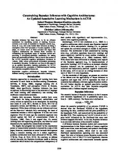
Figure 1: Certainty and gain. (a) The population activity, r, on the left is the single trial response to a stimulus whose value was 70. All neurons were assumed to have a translated copy of the same generic Gaussian tuning curve to s. Neurons are ranked by their preferred stimulus (i.e., the stimulus corresponding to the peak of their tuning curve). The plot on the right shows the posterior probability distribution over s given r, as recovered using Bayes’ theorem (Equations (1) and (2)). When the neural variability follows an independent Poisson distribution (which is the case here), it is easy to show that the gain, g, of the population code (its overall amplitude) is inversely proportional to the variance of the posterior distribution, σ2. (b) Decreasing the gain increases the width of the encoded distribution. Note that the population activity in a and b have the same widths; only their amplitudes are different.
4
variability (and, in fact, for many other noise models, as we discuss below), it is possible to encode any Gaussian probability distribution with population activity. This type of parameterization is sometimes known as a product of experts 16.
A simple case study: multisensory integration P(r1|s)
While it is clear that population activity can represent probability
precisely what we mean by “optimal”. In a cue combination task, the goal is to integrate two cues, c1 and c2, both of which provide information about the same stimulus, s. For instance, s could be the spatial location of a stimulus, c1 could be a visual cue
= Kg1
135
S
g1 0
25 20 15 10 5 0 0
Activity
25 20 15 10 5 0
+
45 90 135 Preferred stimulus
25 20 15 10 5 00
g2 45 90 135 Preferred stimulus P(r2|s)
however, we need to define
C2
Activity
with human behavior? Before asking how neurons can do this,
0.02
P(r1+r2|s)
C1
Activity
inference – in ways consistent
1
σ 12
00
distributions, can they carry out any optimal computations – or
0.04
0.04
1
0.02 0
0
σ S
135
2 2
= Kg 2
1
σ 32
g3=g1+g2
45 90 135 Preferred stimulus
0.04 0.02 0
0
S
135
= Kg 3 = K ( g1 + g 2 ) =
1
σ 12
+
1
σ 22
Figure 2: Inference with probabilistic population codes for Gaussian probability distributions and Poisson variability. The left plots correspond to population codes for two cues, c1 and c2, related to the same variable s. Each of these encodes a probability distribution with a variance inversely proportional to the gains, g1 and g2, of the population codes (K is a constant depending on the width of the tuning curve and the number of neurons).. Adding these two population codes leads to the output population activity shown on the right. This output also encodes a probability distribution with a variance inversely proportional to the gain. Since the gain of this code is g1+g2, and g1 and g2 are inversely proportional to σ12 and σ22, respectively, the inverse variance of the output population code is the sum of the inverse variances associated with c1 and c2. This is precisely the variance expected from an optimal Bayesian inference (Equation (5)). In other words, taking the sum of two population codes is equivalent to taking the product of their encoded distributions.
for the location, and c2 could be an auditory cue. Given observations of c1 and c2, and under the assumption that these quantities are independent given s, the posterior over s is obtained via Bayes’ rule,
p ( s | c1 , c2 ) ∝ p ( c1 | s ) p ( c2 | s ) p ( s ) .
(3)
When the prior is flat and the likelihood functions, p(c1|s) and p(c2|s), are Gaussian with respect to s with means μ1 and μ2 and variances σ12 and σ22, respectively, the mean and variance of the posterior, μ3 and σ32, are given by17 5
σ 22 σ 12 μ3 = 2 μ + μ σ 1 + σ 22 1 σ 12 + σ 22 2 1
σ
2 3
=
1
σ
2 1
+
1
σ 22
.
(4) (5)
Experiments show that humans perform a close approximation to this Bayesian inference – meaning their mean and variance, averaged over many trials, follow Equations (4) and (5) – when tested on cue combination 2,3,18,19. Now that we have a target for optimality – Equations (4) and (5) – we can ask how neurons can achieve it. Again we consider two cues, c1 and c2, but here we encode them in population activities, r1 and r2, respectively, with gains g1 and g2 (Fig. 2). These probabilistic population codes (PPCs) represent two likelihood functions, p(r1|s) and p(r2|s). We also assume (for now) that: 1) r1 and r2 have the same number of neurons, and 2) two neurons with the same index i share the same tuning curve profile; that is, the mean value of both r1i and r2i are proportional to fi(s). What we now show is that when the prior is flat (p(s)=constant), taking the sum of the two population codes, r1 and r2, is equivalent to optimal Bayesian inference. By taking the sum, we mean that we construct a third population, r3 = r1 + r2, which is the sum of r1 and r2 on a neuron-by-neuron basis: r3i=r1i+r2i. If r1 and r2 follow Poisson distributions, so will r3. Therefore, r3 encodes a likelihood function with variance σ32, where σ32 is inversely proportional to the gain of r3. Importantly, the gain of the third population, denoted g3, is simply the sum of the gains of the first two: g3=g1+g2 (Fig. 2). Since gk is proportional to 1/σk2 (k = 1, 2, 3), with a constant of proportionality that is independent of k, this relationship between the gains implies that 1/σ32 =1/σ12 +1/σ22. This is exactly Equation (5). Consequently, the variance of the distribution encoded by r3 is precisely the variance of the posterior distribution, p(s|c1,c2).
General theory and the exponential family of distributions Does the strategy of adding population codes lead to optimal inference under more general conditions, such as non-Gaussian distributions over the stimulus and non-Poisson neural variability? In general, the sum, r3=r1+r2, is Bayes-optimal if p(s|r3) is equal to p(s|r1)p(s|r2) or, equivalently, if p(r1+r2|s) ∝ p(r1|s)p(r2|s). This is not the case for most probability distributions (such as additive Gaussian noise with fixed variance; see Supplementary Material) but, as shown
6
in Supplementary Material, the sum is Bayes-optimal if all distributions are what we call Poisson-like, that is, distributions of the form p ( rk | s, g k ) = φ ( rk , g k ) exp ( h T ( s ) rk )
(6)
where the index k can take the value, 1, 2 or 3, and the kernel h(s) obeys
h′ ( s ) = ∑ −k 1 ( s, g k ) f k′ ( s, g k ) ,
(7)
Σκ is the covariance matrix of rk, and fk' is the derivative of the tuning curves. In the case of independent Poisson noise, identically shaped tuning curves, f(s), in the two populations, and different gains, it turns out that h(s)=log f(s), and φ(rk,gk) = exp(-cgk)Πi exp(rki log gk)/rki! with c a constant. As indicated by Equation 7, for addition of population codes to be optimal, the right hand side of this equation must be independent of both gk and k. Since f´ is clearly proportional to the gain, for the first condition to be satisfied Σk(s,gk) must also be proportional to the gain. This is exactly what is observed in cortex, where it is found that the covariance matrix is proportional to the mean spike count
6,20
, which in turn is proportional to the gain. This applies in particular to
independent Poisson noise, for which the variance is equal to the mean, but is not limited to that distribution. For instance, we do not require that the neurons be independent (i.e. that Σk(s,gk) be diagonal). Also, while we need the covariance to be proportional to the mean, the constant of proportionality does not have to be 1. This is important because how the diagonal elements of the covariance matrix scale with g determines the Fano factor, and values reported in cortex for this scaling are not always 1 (as would be the case for purely Poisson neurons), but instead range from 0.3 to 1.86,20. The second condition, that h'(s) must be independent of k, requires that h(s) be identical, up to an additive constant, in all input layers. This occurs, for instance, when the input tuning curves are identical and the noise is independent and Poisson. When the h(s)’s are not the same, so that h(s) Æ hk(s), addition is no longer optimal, but optimality can still be achieved with linear combinations of activity, i.e. a dependence of the form r3 = A1Tr1+ A2Tr2 (provided the
7
functions of s which make up the components of the hk(s)’s are drawn from a common basis set; See Supplementary Material for details). Therefore, even if the tuning curves and covariance structures are completely different in the two population codes – for instance, Gaussian tuning curves in one and sigmoidal in the other – optimal Bayesian inference can be achieved with linear combinations of population codes. To illustrate this point, in Fig. 3 we show a simulation in which there are three input layers in which the tuning curves are Gaussian, sigmoidal increasing, and sigmoidal decreasing, and the parameters of the tuning curves, such as the widths, slopes, amplitude and baseline activity, vary within each layer (i.e., the tuning curves are not perfectly translation invariant). As predicted, with an appropriate choice of the matrices A1, A2, and A3, (see Supplementary Materials), a linear combination of the input activities, r3 = A1Tr1+ A2Tr2+ A3Tr3 , is optimal. important
property of Equation (6) worth
10 Firing rate (Hz)
emphasizing, is that it imposes no constraint on the shape of the probability
distribution
with
25
8 6
2
5 0
–200 –100 0 100 200 Preferred stimulus
Finally, incorporate
it
is
easy
to
prior distributions.
We encode the desired prior in a population code (using Equation (1)) and add that to the population code representing the likelihood function. This predicts that in an area encoding a prior, neurons should fire before the start of the trial. Moreover, if the prior at a
–200 –100 0 100 Preferred stimulus
200
d
b
0.08 Probability
Spike counts
scheme works for a large class of Gaussian distributions.
15 10
15
distributions over s, not just
20
4
0
respect to s, so long as h(s) forms a basis set. In other words, our
c
a
Activity
Another
10
5
0
0.06 0.04 0.02
–200 –100 0 100 Preferred stimulus
200
0 –60
–40
–20 0 stimulus
20
Figure 3: Inference with non-translation invariant Gaussian and sigmoidal tuning curves. (a) Mean activity in the three input layers. Blue curves: input layer with Gaussian tuning curves. Red curves: input layers with sigmoidal tuning curves with positive slopes. Green curves: input layers with sigmoidal tuning curves with negative slopes. The noise in the curves is due to variability in the baseline, widths, slopes and amplitudes of the tuning curves, and to the fact that the tuning curves are not equally spaced along the stimulus axis. (b) Activity in the three input layers on a given trial. These activities were sampled from Poisson distributions with means as in a. Color legend as in a. (c) Solid lines: mean activity in the output layer. Circles: output activity on a given trial, obtained by a linear combination of the input activities shown in b. (d) Blue curves: probability distribution encoded by the blue stars in b (input layer with gaussian tuning curves). Red-green curve: probability distribution encoded by the red and green circles in b (the two input layers with sigmoidal tuning curves). Magenta curve: probability distribution encoded by the activity shown in c (magenta circles). Black dots: probability distribution obtained with Bayes rule (i.e., the product of the blue and red-green curves appropriately normalized). The fact that the black dots are perfectly lined up with the magenta curve demonstrates that the output activity shown in c encodes the probability distribution expected from Bayes rule.
8
particular spatial location is increased, all neurons with receptive fields at that location should fire more strongly (their gain should increase). This is indeed what has been reported in area LIP 21
and in the superior colliculus 22. One problem with this approach is that the encoded prior will
vary from trial to trial due to the Poisson variability. Whether such a variability in the encoded prior is observed in human subjects is not presently known 5.
Simulations with integrate-and-fire neurons So far, our results rely on the assumption that neurons can compute linear combinations of spike counts, which is only an approximation of what actual neurons do. Neurons are nonlinear devices which integrate their inputs and fire spikes. To determine whether it is possible to perform nearoptimal Bayesian inference with realistic neurons, we simulated a network like the one shown in Fig. 2 but with conductance-based integrate-and-fire neurons. The network consisted of two
Firing rate (Hz)
feedforward connections to the output layer, denoted layer 3. The activity in the input layers formed noisy hills with
both layers). We used different values of the positions of the input hills to simulate cue conflict, as is commonly done in psychophysics experiments. The amplitude of each input hill was determined by the reliability of the cue it encoded: the higher the reliability, the higher the hill, as expected for a PPCs with Poisson-like variability (Fig. 1). The activity in the output layer also formed a hill, which was decoded using a locally optimal linear
8 6 4
0
b Covariance of spike count
4a shows the mean input activities in
10
2
the peak in layer 1 centered at s=86.5 and the peak in layer 2 at s=92.5 (Fig.
c
12
Mean network estimate
a
0
40 80 120 Stimulus Preferred stimulus
160
0.08 0.04 0 0 Pre 90 ferr ed s timu180 0 lus
90 ed ferr e r P
92 90 88 86
d
180 ulus stim
Network variance
input layers, denoted 1 and 2, that sent
86 88 90 92 Mean optimal estimate
8 6 4 2 0
0
2
4 6 8 Optimal variance
Figure 4: Near-optimal inference with a two-layer network of integrate-and-fire neurons similar in spirit to the network shown in Fig. 2. The network consisted of two input layers that sent feedforward connections to the output layer. The output layer contained both excitatory and inhibitory neurons and was recurrently connected; the input layers were purely excitatory and had no recurrent connections. (a) Average activity in the two input layers for identical gains. The positions of the two hills differ on average by 6 to simulate a cue conflict (the units are arbitrary). (b) Covariance matrix of the spike count in the output layer. The diagonal terms (the variances) were set to zero in this plot because they swamp the signal from the covariance (and are uninformative). Because of lateral connections and correlations in the input, output units with similar tuning are correlated. (c) Mean of the probability distribution encoded in the output layer when inputs 1 and 2 are presented together (“Mean network estimate”) versus mean predicted by an optimal Bayesian estimator (“Mean optimal estimate”, obtained from Equation (4); see Methods). Each point corresponds to the means averaged over 1008 trials for a particular combination of gains in the input layers. The symbols correspond to different types of input. Circles: same tuning curves and same covariance matrix for both inputs. Plus signs: same tuning curves, different covariance matrices. Crosses: different tuning curves and different covariance matrices (see Methods). (d) Same as in c but for the variance. The optimal variance is obtained from Equation (5). In both c and d, the data lie near the line with slope one (diagonal dashed line), indicating that the network performs a close approximation to Bayesian inference.
9
estimator23. Parameters were chosen such that the spike counts of the output neurons exhibit realistic Fano factors (Fano factors ranging from 0.76 to 1.0). As we have seen, Fano factors which are independent of the gain are one of the key properties required for optimality. Additionally, the conductances of the feedforward and lateral connections were adjusted to ensure that the average firing rates of the output neurons were approximately linear functions of the average firing rates of the input neurons. Because of the convergent feedforward connectivity and the cortical connections, output units with similar tuning ended up being correlated (Fig. 4b). (See Methods and Supplementary Materials for additional details of the model). The goal of these simulations was to assess whether the mean and variance of the distributions encoded in the output layer are consistent with optimal Bayesian inference (Equations (4) and (5)). To simulate psychophysical experiments, we first presented one cue at a time; that is, we activated either layer 1 or layer 2, but not both. We systematically varied the certainty of the cue by changing the value of the gain of the activated input layer. For each gain, we computed the mean and variance of the distribution encoded in the output layer when only one cue was presented. These were denoted μ1 and σ12, respectively, when only input 1 was active, and μ2 and σ22 when only input 2 was active. We then presented both cues together, which gave us μ3 and σ32, the mean and variance of the distribution encoded in the output layer when both cues are presented simultaneously. To test whether the network was Bayes-optimal, we plotted, in Fig. 4c, μ3 against μ1
σ 22 σ 12 + μ (Equation (4)), and, in Fig. 4d, σ32 2 σ 12 + σ 22 σ 12 + σ 22
σ 12σ 22 against 2 (Equation (5)) over a wide range of values of certainty for the two cues σ 1 + σ 22 (corresponding to gains of the two input hills). If the network is performing a close approximation to Bayesian inference, the data should lie close to a line with slope 1 and intercept 0. As can be seen in Fig. 4c,d, it is clear that the network is indeed nearly optimal on average for all combinations of gains tested, as has been found in human data1-4. This result holds even when the input layers use different sets of tuning curves and different patterns of correlations (Fig. 4d), thus confirming the applicability of our analytical findings. Therefore, linear combinations of probabilistic population codes are Bayes-optimal for Poisson-like noise.
10
Experimental predictions These ideas can be tested experimentally in different domains, since Bayesian inference appears to be involved in many sensory, motor and cognitive tasks. We now consider three specific predictions that can be tested with single- or multi-unit recordings: First, we predict that if an animal exhibits Bayes-optimal behavior in a cue combination task, and the variability of multisensory neurons is Poisson-like (as defined by Equation (6)), one should find that the responses of these neurons to multisensory inputs should be the sum of the responses to the unisensory inputs. This prediction seems at odds with the main result that has been emphasized in the literature, namely, superadditivity. Superadditivity refers to a multimodal response that is greater than the value predicted by the sum of the unimodal responses 24. Recent studies 25,26, however, have shown that the vast majority of multisensory neurons exhibit additive responses in anesthetized animals. What is needed now to test our hypothesis is similar data in awake animals performing optimal multisensory integration. Our second prediction concerns decision making; more specifically, binary decision making (as in 27). In these experiments, animals are trained to decide between two saccades (in opposite directions) given the direction of motion in a random-dot kinematogram. In a Bayesian framework, the first step in decision-making is to compute the posterior distribution over the decision variable, s, given the available evidence. In this particular task, the evidence takes the form of a population pattern of activity from motion sensitive neurons, probably from area MT. Denoting rtMT to be the population pattern of activity in area MT at time t, the posterior distribution over s since the beginning of the trial can be computed recursively using Bayes’ rule, MT p ( s | rtMT ,K , r1MT ) ∝ p ( rtMT | s ) p ( s | rtMT ). −1 , K , r1
(8)
Note that this inference involves, as with cue combination, multiplying probability distributions. Thus, if we represent the posterior distribution at time t-1, p(s|rt-1MT,…, r1MT), in a probabilistic population code (say in area LIP) then, upon observing a new pattern of activity from MT, we can simply add this pattern to LIP activity. In other words, LIP neurons will automatically implement Equation (8) simply by accumulating activity coming from MT. This predicts that LIP neurons behave like neural integrators of MT activity, which is consistent with what Shadlen et al. have found 28. In addtion, this predicts that the profile of tuning curves of LIP 11
neurons over time should remain identical; only the gain and the baseline should change. This prediction has yet to be tested. Third, our theory makes a general prediction regarding population codes in the cortex and their relation to behavioral performance. If a stimulus parameter is varied in such a way that the subject is less certain about the stimulus, the probability distribution over stimuli recovered by Equation (1) (as assumed by PPCs) should reflect that uncertainty (in the case of a Gaussian posterior, for example, the distribution should get wider). This prediction has been verified in two cases in which it has been tested experimentally: motion coherence 29,30 and contrast
31,32
This last prediction may not be valid in all areas of the brain. For instance, it is conceivable that motor neurons encode a single action, not a full distribution over possible actions (as would be the case for any network computing maximum-likelihood estimates, see for instance
33
). If that were the case, applying Bayes’ rule to the activity of motor neurons would
not return a posterior distribution that reflects the certainty of the subject about this action being correct..
DISCUSSION We have argued that the nervous system may use probabilistic population codes (PPCs) to encode probability distributions over variables in the outside world (such as the orientation of a bar or the speed of a moving object). This notion is not entirely novel. Several groups have pointed out that probability distributions can be recovered from neuronal responses through Equation (1)8-10,34. However, we go beyond this observation in two ways. First, we show that Bayesian inference – a nontrivial and critically important computation in the brain – is particularly simple when using PPCs with Poisson-like variability. Second, we do not merely propose that population activity encodes distributions – this part is always true, in the sense that Equation (1) can always be applied to a population code. The novel aspect of our claim is that the probability distributions encoded in some areas of the cortex reflect the uncertainty about the stimulus, while in other areas they do not (in particular in motor areas, as discussed at the end of the previous section). Other types of neural codes beside PPCs have been proposed for encoding probability distributions that reflect observer’s uncertainty3,11,12,28,35-43. In most of these, however, the Poisson-like variability is either ignored altogether, or treated as a nuisance factor that corrupts
12
the codes. In only one of them was Poisson-like variability taken into account, and, in fact, used to compute explicitly the log likelihood of the stimulus43, presumably because log likelihood representations have the advantage that they turn products of probability distributions into sums 28,35,41-43
. A crucial point of our work, however, is to show that, when the neural variability
belongs to the exponential family with linear sufficient statistics (as is the case in43), products turn into sums without any need for an explicit computation of the log likelihood. This is important because there are a number of problems associated with the explicit computation of the log likelihood. For instance, the model described in
43
is limited to independent Poisson noise,
unimodal probability distributions, and winner-take-all readout. This is problematic, as the noise in the cortex is correlated, probability distributions can have multiple peaks (e.g. the Necker cube), and winner-take-all is a particularly inefficient read-out technique. More importantly, the log likelihood approach runs into severe computational limitations when applied to many Bayesian inference problems such as ones involved in Kalman filters
41
. By contrast, the PPC
approach works for correlated Poisson-like noise and a wide variety of tuning curves, the latter being crucial for optimal nonlinear computations extended to Kalman filters
34,44
. Our framework can also be readily
45
. Finally, it has the advantage of being recursive: with PPCs, all
cortical areas use the same scheme to represent probability distributions, (as opposed to log likelihood schemes, in which some areas use the standard tuning curve plus noise model while others explicitly compute log likelihood). Recursive schemes map very naturally onto the stereotyped nature of cortical microcircuitry
46
.
One limitation of our scheme, and of any scheme that reduces Bayesian inference to addition of activities, is that neural activities are likely to saturate when sequential inferences are required. To circumvent this problem, a nonlinearity is needed to keep neurons within their dynamical range. A nonlinearity like divisive normalization 47,48would be ideal because it is near linear for low firing rate, where uncertainty is large and thus there is much to be gained from performing exact inference, and saturating at high firing rate, where uncertainty is small and there is little to be gained from exact inference (see Fig. 1). In conclusion, our notion of probabilistic population codes offers an intriguing perspective on the role of Poisson-like variability. The presence of such variability throughout the cortex suggest that the entire cortex represents probability distributions, not just estimates, which is precisely what would be expected from a Bayesian perspective (see also
49
for related
13
ideas). We propose that these distributions are collapsed onto estimates only when decisions are needed, a process that may take place in motor cortex or in subcortical structures. Interestingly, our previous work shows that attractor dynamics in these decision networks could perform this step optimally by computing maximum-a-posteriori estimates 33.
METHODS Spiking neuron simulations A detailed description of the network is given in Supplementary Materials; here we give a brief overview. The network we simulated is a variation of the model of Series et al.23. It contains two input layers and one output layer. Each input layer consists of 1008 excitatory neurons. These neurons exhibit bell-shaped tuning curves with preferred stimuli evenly distributed over the range [0,180] (stimulus units are arbitrary). The input spike trains are near-Poisson with mean rates determined by the tuning curves. The output layer contains 1260 conductance-based integrate-and-fire neurons, of which 1008 are excitatory and 252 inhibitory. Each of those neurons receives connections from the input neurons. The conductances associated with the input connections follow a Gaussian profile centered on the preferred stimulus of each input unit. The connectivity in the output layer is chosen so that the output units exhibit Gaussian tuning curves whose widths are close to the widths of the convolved input (i.e., the width after the input tuning curves have been convolved with the feedforward weights). The balance of excitation and inhibition in the output layer was adjusted to produce high Fano factors (0.7-1.0), within the range observed in vivo6,20. Finally, additional tuning of connection strengths was performed to ensure that the firing rates of the output neurons were approximately linear functions of the firing rates of the input neurons. We simulated three different networks. In the first (blue dots in Figs. 4c and d), for both populations the widths of the input tuning curves were 20 and the widths of the feedforward weights were 15. In the second (red dots in Figs. 4c and d), the widths of the input tuning curves were 15 and 25 and the widths of the corresponding feedforward weights were 20 and 10. The effective inputs for the two populations had identical tuning curves (with a width of 35) but, unlike in the first network, different covariance matrices. Finally, in the third network (green
14
dots in Figs. 4c and d), the widths of the input tuning curves were 15 and 25 and the width of the feedforward weights was 15. In this case both the tuning curves and the covariance matrices of the effective inputs were different.
Estimating the mean and variance of the encoded distribution To determine whether this network is Bayes-optimal, we need to estimate the mean and variance of the probability distribution encoded in the output layer. In principle, all we need is p(r|s), Equation (1). The response, however, is 1008-dimensional. Estimating a distribution in 1008 dimensions requires an unreasonably large amount of data – more than we could collect in several billion years. We thus used a different approach. The variances can be estimated using a locally optimal linear estimator, as described in Series et al23. For the mean, we fit a Gaussian to the output spike count on every trial and used the position of the Gaussian as an estimate of the mean of the encoded distribution. The best fit was found by minimizing the Euclidean distance between the Gaussian and the spike counts. The points in Figs. 4c and d are the means and variances averaged over 1008 trials (see Supplementary Material for details).
15
REFERENCES 1. 2. 3. 4. 5. 6. 7. 8. 9. 10. 11. 12. 13. 14. 15. 16. 17. 18. 19. 20. 21. 22.
Knill, D. C. & Richards, W. Perception as Bayesian Inference (Cambridge University Press, New York, 1996). van Beers, R. J., Sittig, A. C. & Gon, J. J. Integration of proprioceptive and visual position-information: An experimentally supported model. J Neurophysiol 81, 1355-64. (1999). Ernst, M. O. & Banks, M. S. Humans integrate visual and haptic information in a statistically optimal fashion. Nature 415, 429-33 (2002). Kording, K. P. & Wolpert, D. M. Bayesian integration in sensorimotor learning. Nature 427, 244-7 (2004). Stocker, A. A. & Simoncelli, E. P. Noise characteristics and prior expectations in human visual speed perception. Nat Neurosci 9, 578-85 (2006). Tolhurst, D., Movshon, J. & Dean, A. The statistical reliability of signals in single neurons in cat and monkey visual cortex. Vision Research 23, 775-785 (1982). Stevens, C. F. Neurotransmitter release at central synapses. Neuron 40, 381-8 (2003). Foldiak, P. in Computation and Neural Systems (eds. Eeckman, F. & Bower, J.) 55-60 (Kluwer Academic Publishers, Norwell, MA, 1993). Sanger, T. Probability density estimation for the interpretation of neural population codes. Journal of Neurophysiology 76, 2790-3 (1996). Salinas, E. & Abbot, L. Vector reconstruction from firing rate. Journal of Computational Neuroscience 1, 89-107 (1994). Zemel, R., Dayan, P. & Pouget, A. Probabilistic interpretation of population code. Neural Computation 10, 403-430 (1998). Anderson, C. in Computational Intelligence Imitating Life 213-222 (IEEE Press, New York, 1994). Seung, H. & Sompolinsky, H. Simple model for reading neuronal population codes. Proceedings of National Academy of Sciences. USA 90, 10749-10753 (1993). Snippe, H. P. Parameter extraction from population codes: a critical assessment. Neural Comput 8, 511-29 (1996). Wu, S., Nakahara, H. & Amari, S. Population coding with correlation and an unfaithful model. Neural Computation 13, 775-97 (2001). Hinton, G. E. in Proceedings of the Ninth International Conference on Artificial Neural Network 1-6 ( IEEE, London, England, 1999). Clark, J. J. & Yuille, A. L. Data Fusion for Sensory Information Processing Systems (Kluwer Academic, Boston, 1990). Knill, D. C. Discrimination of planar surface slant from texture: human and ideal observers compared. Vision Research 38, 1683-711 (1998). Gepshtein, S. & Banks, M. S. Viewing geometry determines how vision and haptics combine in size perception. Curr Biol 13, 483-8 (2003). Gur, M. & Snodderly, D. M. High response reliability of neurons in primary visual cortex (V1) of alert, trained monkeys. Cereb Cortex 16, 888-95 (2006). Platt, M. L. & Glimcher, P. W. Neural correlates of decision variables in parietal cortex. Nature 400, 233-8 (1999). Basso, M. A. & Wurtz, R. H. Modulation of neuronal activity by target uncertainty. Nature 389, 66-9 (1997).
16
23. 24. 25. 26. 27. 28. 29. 30. 31. 32. 33. 34. 35. 36. 37. 38. 39. 40. 41. 42. 43.
Series, P., Latham, P. & Pouget, A. Tuning curve sharpening for orientation selectivity: coding efficiency and the impact of correlations. Nature Neuroscience 10, 1129-1135 (2004). Stein, B. E. & Meredith, M. A. The merging of the senses (MIT Press, Cambridge, MA, 1993). Stanford, T. R., Quessy, S. & Stein, B. E. Evaluating the operations underlying multisensory integration in the cat superior colliculus. J Neurosci 25, 6499-508 (2005). Perrault, T. J., Jr., Vaughan, J. W., Stein, B. E. & Wallace, M. T. Superior colliculus neurons use distinct operational modes in the integration of multisensory stimuli. J Neurophysiol 93, 2575-86 (2005). Shadlen, M. N. & Newsome, W. T. Neural basis of a perceptual decision in the parietal cortex (area LIP) of the rhesus monkey. J Neurophysiol 86, 1916-36 (2001). Gold, J. I. & Shadlen, M. N. Neural computations that underlie decisions about sensory stimuli. Trends in Cognitive Sciences 5, 10-16 (2001). Britten, K. H., Shadlen, M. N., Newsome, W. T. & Movshon, J. A. Responses of neurons in macaque MT to stochastic motion signals. Vis Neurosci 10, 1157-69 (1993). Weiss, Y. & Fleet, D. J. in Statistical Theories of the Cortex (eds. Rao, R., Oshausen, B. & Lewicki, M. S.) (MIT Press, Cambridge, 2002). Anderson, J. S., Lampl, I., Gillespie, D. C. & Ferster, D. The contribution of noise to contrast invariance of orientation tuning in cat visual cortex. Science 290, 1968-72 (2000). Sclar, G. & Freeman, R. Orientation selectivity in the cat's striate cortex is invariant with stimulus contrast. Experimental Brain Research 46, 457-61 (1982). Deneve, S., Latham, P. & Pouget, A. Reading population codes: A neural implementation of ideal observers. Nature Neuroscience 2, 740-745 (1999). Deneve, S., Latham, P. & Pouget, A. Efficient computation and cue integration with noisy population codes. Nature Neuroscience 4, 826-831 (2001). Barlow, H. B. Pattern recognition and the responses of sensory neurons. Ann N Y Acad Sci 156, 872-81 (1969). Simoncelli, E., Adelson, E. & Heeger, D. in Proceedings 1991 IEEE Computer Society Conference on Computer Vision and Pattern Recognition 310-315 (1991). Koechlin, E., Anton, J. L. & Burnod, Y. Bayesian inference in populations of cortical neurons: a model of motion integration and segmentation in area MT. Biol Cybern 80, 25-44 (1999). Anastasio, T. J., Patton, P. E. & Belkacem-Boussaid, K. Using Bayes' rule to model multisensory enhancement in the superior colliculus. Neural Computation 12, 1165-87 (2000). Hoyer, P. O. & Hyvarinen, A. in Neural informatoin processing systems (MIT Press, 2003). Sahani, M. & Dayan, P. Doubly distributional population codes: simultaneous representation of uncertainty and multiplicity. Neural Comput 15, 2255-79 (2003). Rao, R. P. Bayesian computation in recurrent neural circuits. Neural Comput 16, 1-38 (2004). Deneve, S. in Neural Information Processing System (MIT Press, 2005). Jazayeri, M. & Movshon, J. A. Optimal representation of sensory information by neural populations. Nat Neurosci 9, 690-6 (2006).
17
44. 45. 46. 47. 48. 49.
Poggio, T. A theory of how the brain might work. Cold Spring Harbor Symposium on Quantitative Biology 55, 899-910 (1990). Beck, J., Ma, W. J., Latham, P. E. & Pouget, A. in Cosyne abstracts (Salt Lake City, 2006). Douglas, R. J. & Martin, K. A. A functional microcircuit for cat visual cortex. J Physiol 440, 735-69 (1991). Heeger, D. J. Normalization of cell responses in cat striate cortex. Visual Neuroscience 9, 181-197 (1992). Nelson, J. I., Salin, P. A., Munk, M. H., Arzi, M. & Bullier, J. Spatial and temporal coherence in cortico-cortical connections: a cross-correlation study in areas 17 and 18 in the cat. Vis Neurosci 9, 21-37 (1992). Huys, Q., Zemel, R. S., Natarajan, R. & Dayan, P. Fast population coding. Neural Computation (In press).
18