providing maximum economic benefit throughout the life cycle. Calculating life cycle ..... are failures of the class broken and in this case the highest spare part ...
Bayesian Nets for Life Cycle Cost Forecasting Danina Janz1, Stefan Schneider1, Michael Kempf1, Engelbert Westkämper1 1 Department of Product and Quality Management, Fraunhofer Institute for Manufacturing Engineering and Automation (IPA), Stuttgart, Germany Abstract Plant and system operators are looking for reliable products meeting high technical requirements while providing maximum economic benefit throughout the life cycle. Calculating life cycle costs different operating conditions have to be considered to provide reliable decision making assistance. If data for a direct probability measurement may not be available, expert knowledge needs to be considered. The model presented enables a combination of expert knowledge and collected lifetime data to be used for estimating product operational costs. Modelling costs this way, the plausibility of a given statement can be updated in the light of new information to produce a more accurate cost estimation. Keywords Life cycle costing, Availability, Bayesian Networks
calculation of life cycle costs has to predict future costs as accurately as possible in order to provide reliable decision making assistance. Traditional cost probability calculus is based on past data where probability is derived from directly observed or assumed frequency distributions. Sometimes the probability of an event (failure or cost relevant resource consumption) can be measured directly. But at other times, the data for such measurement may not be available and we will need to rely initially on probabilities elicited from experts. These numerical parameters are not, however, the sole components of a knowledge and cost estimating model. There will always be some structure to the influences between variables in the cost estimating model. In order to set up a cost forecasting model which uses all sources of information available and considers expert judgement as a starting point we chose the Bayesian Networks as instrument. There is a closed relation between the availability and reliability of products or systems during their operational phase and the life cycle costs incurred. In order to obtain reliability statements of manufacturing machinery and equipment, tools like failure mode and effects analysis (FMEA) and fault tree analysis (FTA) are used. As not every failure causes an interruption of operation the reliability structure (identification of reliability dependencies between system and components) has to be analysed. Modelling and calculating reliability is a probabilistic task. Taking additional influences, and dependencies respectively, into account leads to conditional probabilities. There is a distinction to be made between predicted and estimated reliability. The first one is calculated on the basis of the item’s reliability structure and the failure rate of its components, the second is obtained from statistical evaluation of reliability tests or from field data by known environmental and operating conditions. Whenever a statement of the probability P(a) of an event a is given, then it is given conditioned on other known factors.[1] The mathematical discipline corresponding to conditional probabilities is the Bayesian probability calculus with its implementation tool Bayesian (Belief) Networks (BBN/BN).
1 INTRODUCTION Life Cycle Costing is currently an often discussed topic in the manufacturing engineering because of the growing need to quantify full product costs, including also costs associated with installation, regular maintenance and periodic replacement in order to support investment decisions. Life cycle costs are mainly determined by decisions taken during the early product life cycle phases – concept, development & design - but they actually occur in the later phases – build & install, operation/support, conversion and/or decommission and disposal -. This paper focuses on capital goods and on costs during the operation phase. Key factors affecting these costs are product’s quality and availability during operation. Since failures during the operation phase are influencing the number of spare parts and maintenance/support activities needed, calculating life cycle costs one can not afford to ignore aspects of availability and reliability. Modern and highly automated product systems are growing in complexity. The opposite trend is the use of various instances of specific components and subsystems within the same product system. Often these components can perform their required functions under different operating conditions (e.g. positions, speed, accuracy, stress intensity, etc.) In this paper we will introduce an approach of modelling availability as well as life cycle costs of a specified product system, for example a special type of machine, in regard to its operational settings and the required tasks. As the description of the operational setting might not in general be available and/or expressible in technical terms we make use of a probabilistic type of models, namely Bayesian Networks. They cover both necessary aspects of system modelling: causality and probabilistic modelling to express the influences of the operational setting. The approach uses common methods of reliability and availability analysis for modelling and simulating system availability and operational costs. The goal of the current approach is to develop a technique to enable a combination of expert knowledge and collected field data to be used to develop and further refine a life cycle cost estimating model. 2
CALCULATION OF LIFE CYCLE COSTS CONSIDERING AVAILABILITY Life cycle costing helps to quantify full product costs, including additional costs associated with installation, regular maintenance and periodic replacement, making it possible to select the most economic alternative. The
2.1 Cost model considering availability and operating conditions The cost model focuses on the prediction of operational costs incurred by operation conditions and the availability and reliability of the considered system. Availability as a property of manufacturing systems is the crucial factor on
687
the productivity of the overall manufacturing line. Reliability and availability of manufacturing systems are not static properties. The required amount of output (productivity) of the manufacturing system has obvious effect hereon. The productivity requirements can be interpreted as operating conditions of the overall manufacturing system. On the one hand, modern, highly automated manufacturing systems are growing in complexity. On the other hand, there are various instances of specific components or subsystems in the same manufacturing system. At this subsystem level a productivity requirement of the overall system leads to different operating conditions of each subsystem instance (consider e.g. machines performing similar tasks with different speed, accuracy, stress intensity, position, etc.). Operating conditions have an important influence upon reliability, and must therefore be specified with care [1]. A higher failure rate has to be expected when the system is operating close to its capacity limit. The immediate consequences are a higher number of maintenance activities and of spare parts, with other words higher operational costs. The natural ability of BN to cope with dependency structures is regarded as a major advantage over existing reliability and cost prediction techniques. As this model is a Bayesian Network it is capable to receive input (evidence to the BN) about the states of the operating conditions, as a vector OC. This evidence is used on the one hand to compute the resulting probability of a system S’ ∈ S being in the state system down, conditioned on k S’ S’ operating conditions OCk as P(S=up / OCk ). On the other hand this evidence is used to compute the probability of the costs incurred by the considered k operating conditions lying within an estimated interval [x1, S x2] as P(S = [x1,x2] / OCk ). The operational cost estimation model integrates as a subsystem an availability prediction BN and uses the output of this subsystem for prediction of maintenance actions, their duration and derives from this the incurred costs. Furthermore the availability subnet is used for prediction of the number of spare parts needed. The BN for the prediction of availability has been developed at Fraunhofer IPA in a precedent paper and is used within this approach as subnet of the cost prediction net [2]. The approach focuses on prediction of the costs involved by direct resource consumption, like energy, lubricants, maintenance time and personal capacity. It does not support the estimation of time values for prices for the resources consumed. 2.2 Bayesian (Belief) Networks Bayesian Belief Networks (BNN/BN) are used to provide a compact visualisation of the concept of conditional probabilities. The basic definitions are adopted from R.F. Jensen [2]. It should be stated that the probability P(a) of an event a is understood as a number in the unit interval [0,1] obeying the following basic axioms: (i) P(a) = 1 if and only if a is certain (ii) If a and b are mutually exclusive, then: P(a ∧ b) = P(a) + P(b). A conditional probability statement is of the following kind: “Given the event b, the probability of the event a is x.” and the notation of the preceding statement is P(a/b) = x. The fundamental rule for the probability calculus is P(a/b)P(b) = P(a,b), (1)
688
where P(a,b) is the probability of the joint event a ∧ b. Remembering that probabilities should always be conditioned on a context c, the formula should read: P(a/b,c)P(b/c) = P(a,b/c). (2) From (1) follows P(a/b)P(b) = P(b/a)P(a), and this yields the Bayes’ rule: P(b/a) =
P (a / b) P(b) P(a)
(3)
Bayes’ rule conditioned on c reads:
P(a / b, c) P (b / c ) P(a / c)
P(b/a,c) =
(4)
In general a Bayesian Network (BN) is a causal model of the world it describes. It is a combination of two parts: qualitative (representing the causal structure via variables standing for systems or components for example) and quantitative (representing the probability relations of the systems being in different states) [3]. A Bayesian network is defined as consisting of the following: •
A set of variables and a set of directed edges between variables.
•
Each variable has a finite set of mutually exclusive states.
•
The variables together with the directed edges form a directed acyclic graph (DAG). (A directed graph is acyclic if there is no directed path A1 Æ…ÆAn so that A1 =An).
•
To each variable A with parents B1,…Bn there is attached the probability table P(A / B1,…,Bn). It has to be noted that if a has no parents, then the table reduces to unconditional probabilities P(A). for the DAG in figure 1, the prior probabilities P(A) and P(B) must be specified [4]. The chain rule for Bayesian Networks defines BN as a Bayesian Network over the universe of variables U = {A1 ,..., An }. Then, the joint probability distribution P(U) is the product of all potentials (probability tables) specified in the BN
P (U ) =
∏ P( Ai / pa( Ai ))
(5),
i
where pa(Ai) is the parent set of Ai. 2.3 Learning Bayesian Networks Various methods exist for learning with Bayesian Networks including both structural (edges and their directions within the BN) and parameter (values of the conditional probability tables (CPTs) learning from data [5]. In our approach to availability and cost modelling only parameter learning is of interest. In this case the structure is known and data is obtainable on all variables of the network. BN can also cope with incomplete data, when the network structure is known, but this is a specific situation not focused within this paper. For illustrating the general idea of parameter learning we assume that learning data for a BN node X is like finding of a statistical experiment about the frequency with which a corresponding random variable X is in its two different states x1 or x2 (here considered binary).
P ROCEEDINGS OF LCE2006
A
•
B
Its functional complexity suggests a system theoretic modelling (reparable system with different possible failure sources)
•
C D F
E G
Figure 1: Directed Acyclic Graph (DAG). The intuitive value for the probability of P(X=x1) would be the relative frequency for X = x1 within the experiment.
P ( X = x1 ) =
numberofcases( X = x1 ) numberofobservationsforX
(6)
BN learning algorithms in general assign a probability distribution to each node which expresses the characteristics of its corresponding learning data. The distribution is then used to estimate the probability table of the nodes (which in the binary cases equals the equation above). When learning from new cases this distribution is updated accordingly and the probability table of the correspondent BN node is recalculated. Most learning algorithms allow to weight new cases statistically by assigning an experience value or case count. This allows expressing a higher belief in certain observations. Thereby the experience and case counts are specific to the learning case and not to the nodes they contain evidence. If the probability tables contain values before learning is performed (initial probability tables are specified) the learning algorithm incorporates those according to their experience count. If this is equal to zero they are ignored and overwritten after when the learning cases contain appropriate evidence. The existing algorithms differ in their approaches to the distribution functions (beta distribution is common for binary nodes while a Dirichlet distribution is used in the multi-state case). The Estimation Maximisation (EM) algorithm and its extensions are able to cover problems of missing data or support even structural learning methods [6]. We use the term complete learning of a BN if for each node in the BN and for all its columns in the conditional probability table which correspond to the parents’ state combinations at least on learning case is available. 3
STRUCTURE OF THE BAYESIAN NETWORK INCLUDING OPERATING CONDITIONS To illustrate the structure of the Bayesian Network including operating conditions let us consider the example of three manufacturing machines: mac1, mac2 and mac3. The three machines are of the same kind and the system class S is assumed to be this type of machine. For the general idea of modelling availability and costs including operating conditions the following restrictions on instances (elements) of the examined system class S have to be applied: •
The system classified in S has a large application field and is therefore used in many different operation settings.
Operation settings of the system are identifiable by a number nOC of operating conditions (nOC of manageable size). These restrictions seem very weak as limiting quantities are not very strict. The first restriction can also be paraphrased as the imperative of the ability to perform different required tasks or similar ones in different speeds, for example. As Bayesian Networks tend to become complex for many variables the third assumption is made. In practice, the quantitative limitation of available data to learn the probabilities of the Bayesian Networks influences the complexity of the model. For restriction 3, nOC ≤ 3 can roughly serve as a quantitative expression. Manufacturing machines generally tend to be used in different operating settings. The operating conditions which were assumed show that these machines are capable of performing their required tasks with different speeds. Therefore restriction one is fulfilled. If repair actions, differing in duration and costs, on different failures are considered than restriction 2 is also met. Two varying operating conditions guarantee a Bayesian Network of manageable complexity. The diverse operation settings of the three machines are summarised in table 1. Label
operating condition
mac1
mac2
mac3
OCDW
drilling holes
9
4
8
OCTL
time limit
6 min
3 min
5,5 min
Table 1: Diverse operation settings of the machines. 3.1 Implementation of the system structure As a first approximation to the Bayesian Network the system structure is analysed in an object-oriented meaning. Our system class S (a special machine type, furthermore abiding by the example) is decomposed into its subsystems. For our example we have chosen two main components: the drill head (C1) and motion component (C2). The set of possible failures for a given system or subsystem can often be divided in failure classes. Some possible properties for such a distinction are by failure mode, effect or cause. If such a differentiation is possible and the failure cases received from lifetime data can be classified accordingly, one might add additional nodes to the BN. Performing this task depends on the desired expressiveness of the BN. The different failure classes are treated with different maintenance activities and the information on the occurrence probability of the failure classes is of interest due to spare part and personal costs involved in maintenance actions. For illustration purposes we add two failure classes to the BN-node C1 (drill head) and C2 (motion component): uptight (FC1) and broken (FC2). The corresponding maintenance actions are: loosing of deadlock (M1) (for failure case: uptight) and substitution of the drill head (M2) (for failure case: broken). In order to take into consideration failures which are not caused by failure class FC1 and FC2 two additional nodes have been added: C1_1 and C2_2. Further on there are nodes representing the number of spare parts needed for the drill head and for the motion component. The number of spare parts has a direct influence on the spare part costs. For illustration of the further costs incurred by resource consumption the
13th CIRP I NTERNATIONAL C ONFERENCE ON L IFE C YCLE E NGINEERING
689
following nodes have been included: maintenance time (MT), energy consumption (E) and lubricant consumption (L). On cost level there are the nodes: spare part costs (SP_C), personal costs (P_C), energy costs (E_C) and lubricant costs (L_C). The following figure 2 shows the structure of the Bayesian Network including the aforementioned nodes.
OCDW
C1_1
FC1
C1
FC2
C2
OCTL
C2_2
M1
S_A
SP_C1
E
M2
L
MT
SP_C2
SP_C
P_C
E_C
L_C
Co_T Figure 2: Structure of the BN. 3.2 Learning strategy for the Bayesian Network The complete Bayesian Network includes initial probability tables. There are three different types of values (not deterministic) to be determined: the values of probability tables for the nodes representing operating conditions, P(OCk) the probability tables for the failure classes which are conditioned on the operating
(
conditions, P FC j -
Ci
/ OC k
)
the probability tables for the energy and lubricant consumptions which are conditioned on the operating conditions, P(E/OCk) and P(L/OCk) All other values within the probability tables of the BN are specified by the mapped structure. The learning procedure of BN software uses data sets or cases. Dependent on the learning algorithm they can represent evidence, findings or Likelihood evidence to the BN. As resource consumption entry within the system corresponds to the statement “the corresponding BN node is in the interval [x1, x2]”, the cases for our learning strategy contain appropriate evidence. Also do the cases for learning availability data as a failure entry corresponds to the statement “the corresponding BN node is in the state “down”. The BN will learn from resource consumption data as well as from availability data. The probability tables for the operating conditions P(OCk) should represent the state distribution of the set of instances that is used for learning. As the experience count in our learning strategy corresponds respectively to the observed failure free operating time, the time to repair and resource consumption, the probability tables of the
690
operating conditions are to be set manually after learning from data. 3.3 Initialising the Bayesian Network Initialising the BN means to estimate the initial probabilities tables that are not set as deterministic, before any learning procedure is started. This has to be performed if a complete learning is impossible. If not enough learning data is available for a complete learning the initial probability tables can be annotated with experience count equal to zero which ensure that they keep their deterministic probability when learning. For tables conditioned on operating conditions we suggest to initialise with the mean of the available lifetime data. Consider for example a failure class FC being conditioned on two operating conditions. The corresponding probability table P(FC / OC1, OC2) then is 4*4 = 16 columns (each OC having the suggested four states high, rather_high, rather_low and low). The necessary number of observed instances to learn all columns would be even greater because all state combinations have to be covered. In realistic applications it has to be expected that the number of observed instances it much lower. For operating condition nodes initialising with an equal distribution is adequate [7]. 3.4 Prediction Algorithm For a clear illustration of our understanding of the prediction algorithm which can be performed with the BN obtained via our modelling strategy consider the process description showed in figure 3. The following systematic steps shall illustrate the support that a general Bayesian availability and cost model can offer to the subprocess entitled “recalculate MTBF, MTTR and operational costs”: 1. Create appropriate BN learning cases for new failures and resource consumption observed. 2. Start BN learning algorithm. 3. Propagate “learned” BN and output availability values and cost intervals. Application Programming Interfaces (APIs) of a BNsoftware offer to incorporate these steps within a software realisation of the suggested expert system. The modelling approach described in this paper offers a possibility to calculate an updated steady-state value of the point availability and of the costs incurred. If updated predictions of MTBF and MTTR or operational costs are of interest a calculation of these values in regard to the expert guesses is necessary using the cases saved in the data warehouse. 4 NECESSARY PRELIMINARY INVESTIGATIONS For our modelling strategy for a Bayesian Network of a system class including operating conditions as illustrated before, we started with the assumption that knowledge about the systems structure and about the operating conditions is given. 4.1 Structural system analysis The knowledge about the system structure required for our approach consists of information on technological and cost related dependencies between the defined system variables as well as knowledge about failure propagation and maintenance actions. This structural analysis is generally performed top down and has to take expert knowledge into account. Auxiliary methods to gather information about required system parameters are cost breakdown structures, Reliability Block Diagrams (RBD), Failure Mode and Effect Analysis (FMEA) and Fault Tree Analysis (FTA).
P ROCEEDINGS OF LCE2006
verification/update process
data on failures (MTBF, MTTR), resource consumption
data warehouse
recalculation MTBF, MTTR, costs
data warehouse
Figure 3: Verification/update process description. 4.2 Analysis of the Operating Conditions Additional to a structural availability analysis of the system which might be performed anyway, it is necessary to identify the operating conditions of the examined system class. The set of operating conditions answers the purpose to describe the different operational settings. A fist step to identify those variables might be a brainstorming of development, manufacturing and maintenance engineers as well as of controlling experts in which all possible operating conditions OCk are suggested. In the second phase of this brainstorming process the number of operating conditions is to cut down to the necessary ones for describing different operational setting of instances of the examined system class. Finally a number of operating conditions less equal five should be accomplished nOC ≤ 3. Once the set of operating conditions is identified the knowledge of the attendant experts should be used to determine the dependency relations of the operating conditions to components and failure classes, respectively. It is of interest to the simplicity of the Bayesian Network to collect as many as possible statements of kind: operating condition I has no influence on the occurrence probability of failures of a specific failure class. That is to reduce edges from operating condition nodes to failure class or further nodes. To each observed instance of the examined system class an instantiation of the operating conditions is to attach. Therefore a mapping of the states of the operation condition node within the BN (high, rather_high, rather_low, low) to observable values at the instance is to develop within the experts discussion. 4.3 Data retrieval Manufacturing Execution Solutions / systems (MES), Production Planning Systems (PPS) and Enterprise Resource Planning (ERP) solutions are currently growing fields of research to develop manufacturing and operating planning and control. Software solutions in this field may serve as data sources for our approach as they collect system data on the shop floor level, hence for example failure and resource consumption data. A pre-processing can ensure that the available data meets the requirements formulating when modelling the BN. As learning data we used SAP maintenance data. Using SAP maintenance entries we had to include some additional recalculating steps in order to obtain the needed observations for the BN. For example SAP maintenance data including resource consumption and cost relevant details are collected by manual input and it is not guaranteed that they equal the failure event or resource consumption they shall describe. The manual
input of the maintenance entries may lead to inconsistent entries concerning the time values and the assignment to components and spare parts within the system hierarchy. Regarding time inconsistency the maximum error when solving them under considerations of plausibility is less than one percent concerning the mean values MTBF and MTTR. If failures are obviously not assigned to a plausible component our modelling strategy offers an assignment on a higher level in the system hierarchy. This is ensured by the nodes C1_1 and C2_2. 5 RESULTS AND DISCUSSION With the Bayesian Network being completed we performed propagations of the operational costs. The results are shown in figure 4. The model represents the operational costs and system availability given different states for the operational conditions. The drill head can be identified as the most probable cause for the machine to fail because its availability value is lower in comparison to the other component. The most likely causes for the drill head to fail are failures of the class broken and in this case the highest spare part costs are incurred. The failure class uptight implies the most maintenance time and causes the most personal costs. These results are proved by common analysis methods. As the Bayesian Network is a model of the machine system class S it can be used to compare the availability and operational cost of different items of the considered class. The considered example system shows that under similar operating conditions the operational costs of the three machines differ just slightly. Considering different operating conditions the effects on the operational costs and availability aspects became evident. The BN offers within the planning process the possibility to vary the operational settings for a specific instance or to change the number of instances of the considered system class. This way the cost forecasting for the whole system can be optimised and the effects of operating conditions of costs and availability can be better described. This contribution can effectively support decision-making regarding product planning and design, investment and life cycle costing.
13th CIRP I NTERNATIONAL C ONFERENCE ON L IFE C YCLE E NGINEERING
691
up down
Co_T interval1 56.4 interval2 43.6 1.6e+003 ± 1.5e+003
S_A 51.4 48.6
up down
C1 47.6 52.4
up down
C2 73.8 26.2
true false
FC1 63.1 36.9
true false
FC 2 56.5 43.5
true false
C1_1 61.2 38.8
true false
C2_2 37.4 62.6
SP_C interval1 55.4 interval2 44.6 1.5e+002 ± 1.7e+002
interval1 interval2
SP_C1 43.6 56.4 2.8 ± 2.5
true false
M1 39.7 60.3
P_C interval1 45.2 interval2 54.8 6.5e+002 ± 6.3e+002
interval1 interval2
SP_C2 44.7 55.3 1.9 ± 1.5
true false
M2 61.5 38.5
interval1 interval2
E_C 83.1 16.9 48 ± 30
interval1 interval2
L_C 53.3 46.7 145 ± 86
M_T interval1 22.5 interval2 77.5 10.2 ± 4.1
E interval1 67.4 interval2 32.6 1.8e+002 ± 1.4e+002 L interval1 38.4 interval2 61.6 2.3e+002 ± 1.5e+002
OC_DW low 10.0 rather low 10.0 rather high 50.0 high 30.0 4 ± 0.89
low rather low rather high high
OC_TL 32.4 21.5 23.6 22.5
Figure 4: Results of the example Bayesian Network [5] REFERENCES [1] Birolini, A., 2004, Reliability Engineering; Theory and Practice, Springer, Berlin. [2] Schneider, S., 2005, Availability of Technical Systems under Different Operating Conditions – a Bayesian Approach, Project Thesis, IFF, Stuttgart. [3] Jensen, F.V., 1996, An Introduction to Bayesian Networks, Springer, New York. [4] Jensen, F.V., 2001, Bayesian Networks and Decision Graphs, Springer, New York.
692
[6] [7]
[8]
Neapolitan, R.E., 2003, Learning Bayesian Networks, Prentice Hall, New York. Krause, P.J., 1998, Learning Probabilistic Networks, Philips Research Laboratories, Redhill. Kim, J., Pearl, J.A., 1983, A computational model for causal diagnostic reasoning in inference systems, Proceedings of the Eight International Joint Conference on Artificial Intelligence, 190-193. Shafer, G.R., Pearl, J., 1990, Readings in Uncertain Reasoning, Morgan Kaufmann, San Mateo, CA.
P ROCEEDINGS OF LCE2006