Bayesian Network Approach to Multinomial ... - Bayes-Knowledge

Bayesian Network Approach to Multinomial Parameter Learning using Data and Expert Judgments Yun Zhoua,b,∗, Norman Fentona , Martin Neila a Risk

and Information Management (RIM) Research Group, Queen Mary University of London b Science and Technology on Information Systems Engineering Laboratory, National University of Defense Technology

Abstract One of the hardest challenges in building a realistic Bayesian Network (BN) model is to construct the node probability tables (NPTs). Even with a fixed predefined model structure and very large amounts of relevant data, machine learning methods do not consistently achieve great accuracy compared to the ground truth when learning the NPT entries (parameters). Hence, it is widely believed that incorporating expert judgments can improve the learning process. We present a multinomial parameter learning method, which can easily incorporate both expert judgments and data during the parameter learning process. This method uses an auxiliary BN model to learn the parameters of a given BN. The auxiliary BN contains continuous variables and the parameter estimation amounts to updating these variables using an iterative discretization technique. The expert judgments are provided in the form of constraints on parameters divided into two categories: linear inequality constraints and approximate equality constraints. The method is evaluated with experiments based on a number of well-known sample BN models (such as Asia, Alarm and Hailfinder ) as well as a real-world software defects prediction BN model. Empirically, the new method achieves much greater learning accuracy (compared to both state-of-the-art machine learning techniques and directly competing methods) with much less data. For example, in the software defects BN for a sample size of 20 (which would be considered difficult to collect in practice) when a small number of real expert constraints are provided, our method achieves a level of accuracy in parameter estimation that can only be matched by other methods with much larger sample sizes (320 samples required for the standard machine learning method, and 105 for the directly competing method with constraints). Keywords: Bayesian networks, Multinomial parameter learning, Expert judgments ∗ Corresponding

author Email addresses: [email protected] (Yun Zhou), [email protected] (Norman Fenton), [email protected] (Martin Neil)

Preprint submitted to International Journal of Approximate Reasoning

February 17, 2014

2

1. Introduction Bayesian Networks (BNs) [1, 2] are the result of a marriage between graph theory and probability theory, which enable us to model probabilistic and causal relationships for many types of decision-support problems. A BN consists of a directed acyclic graph (DAG) that represents the dependencies among related nodes (variables), together with a set of local probability distributions attached to each node (called a node probability table - NPT - in this paper) that quantify the strengths of these dependencies. BNs have been successfully applied to many real-world problems [3]. However, building realistic and accurate BNs (which means building both the DAG and all the NPTs) remains a major challenge. For the purpose of this paper, we assume the DAG model is already determined, and we focus purely on the challenge of building accurate NPTs. In the absence of any relevant data NPTs have to be constructed from expert judgment alone. Research on this method focuses on the questions of design, bias elimination, judgments elicitation, judgments fusion, etc. (see [4, 5] for more details). At the other extreme NPTs can be constructed from data alone, whereby a raw dataset is provided in advance, and statistical based approaches are applied to automatically learn each NPT entry. In this paper we focus on learning NPTs for nodes with a finite set of discrete states. For a node with ri states and no parents, its NPT is a single column whose ri cells corresponding to the prior probabilities of the ri states. Hence, each NPT entry can be viewed as a parameter representing a probability value of a discrete distribution. For a node with parents, the NPT will have qi columns corresponding to each of the qi instantiations of the parent node states. Hence, such an NPT will have qi different ri -value parameter probability distributions to define or learn. Given sufficient data, these parameters can be learnt, for example using the relative frequencies of the observations [6]. However, many real-world applications have very limited relevant data samples, and in these situations the performance of pure data-driven methods is poor [7]; indeed pure data-driven methods can result in poor results even when there are large datasets [8]. In such situations incorporating expert judgment improves the learning accuracy [9, 10]. It is the combination of (limited) data and expert judgment that we focus on in this paper. A key problem is that it is known to be difficult to get experts with domain knowledge to provide explicit (and accurate) probability values. Recent research has shown that experts feel more comfortable providing qualitative judgments and that these are more robust than their numerical assessments [11, 12]. In particular, parameter constraints provided by experts can be integrated with existing data samples to improve the learning accuracy. Niculescu [13] and de Campos [14] introduced a constrained convex optimization formulation to tackle this problem. Liao [15] regarded the constraints as penalty functions, and applied the gradient-descent algorithm to search the optimal estimation. Chang [16, 17] employed constraints and Monte Carlo sampling technology to reconstruct the hyperparameters of Dirichlet priors. Corani [18]

3

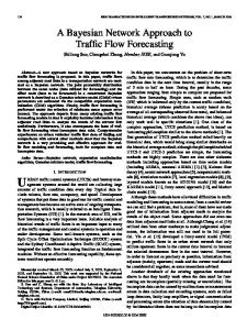
proposed the learning method for Credal networks, which encodes range constraints of parameters. Khan [19] developed an augmented Bayesian network to refine a bipartite diagnostic BN with constraints elicited from expert’s diagnostic sequence. However, Khan’s method is restricted to special types of BNs (two-level diagnostic BNs). Most of these methods are based on seeking the global maximum estimation over reduced search spaces. A major difference between the approach we propose in this paper and previous work is in the way to integrate constraints. We incorporate constraints in a separate, auxiliary BN, which is based on the multinomial parameter learning (MPL) model. Our method can easily make use of both the data samples and extended forms of expert judgment in any target BN; unlike Khan’s method, our method is applicable to any BN. For demonstration and validation purposes, our experiments (in Section 4) are based on a number of well-known and widely available BN models such as Asia, Alarm and Hailfinder, together with a real-world software defects prediction model. To illustrate the core idea of our method, consider the simple example of a BN node (without parents) VA (“Visit to Asia?”) in Figure 1. This node has four states, namely “Never”, “Once”, “Twice” and “More than twice” 1 and hence its NPT can be regarded as having four associated parameters P1 , P2 , P3 and P4 , where each is a probability value of the probability distribution of node VA. Whereas an expert may find it too difficult to provide exact prior probabilities for these parameters (for a person entering a chest clinic) they may well be able to provide constraints such as: “P1 > P2 ”, “P2 > P3 ” and “P3 ≈ P4 ”. These constraints look simple, but are very important for parameter learning with small data samples. Figure 1 gives an overview of how our method estimates the four parameters with data and constraints (technically we only need to estimate 3 of the parameters since the 4 parameters sum to 1). Firstly, for the NPT column of the target node (dashed callout in Figure 1), our method generates its auxiliary BN, where each parameter is modeled as a separate continuous node (on scale 0 to 1) and each constraint is modeled as a binary node. The other nodes correspond to data observations for the parameters - the details, along with how to build the auxiliary BN model - are provided in Section 3. It turns out that previous state-of-the-art BN techniques are unable to provide accurate inference for the type of BN model that the auxiliary BN is. Hence, we describe a novel inference method and its implementation. With this method, after entering evidence, the auxiliary BN can be updated to produce the posterior distributions for the parameters. Finally, the respective means of these posterior distributions are assigned to entries in the NPT. A feature of our approach is that experts are free to provide arbitrary constraints on as few or as many parameters as they feel confident of. Our results show that we get greatly improved learning accuracy even with very few expert constraints provided. The rest of this paper 1 In the Asia BN the node “Visit to Asia” actually only has two states. We are using 4 states here simply to illustrate how the method works in general.

4

VA Visit to Asia? NPT

0

VA Never Once Twice More than twice

P P1 P2 P3 P4

C1

C2

C3

P1

P2

P3

1

0

1

0

1

P4 0

1

Auxiliary BN

Figure 1: The overview of parameter learning with constraints and data. The constraints are: C1: P1 > P2 , C2: P2 > P3 and C3: P3 ≈ P4 . The gray color nodes represent part of the MPL model.

is organized as follows: Section 2 discusses the background of parameter learning for BNs, and introduces related work of learning with constraints; Section 3 presents our model, judgment categories and inference algorithm; Sections 4 describes the experimental results and analysis; Section 5 provides conclusions as well as identifying areas for improvement. 2. Preliminaries In this section we provide the formal BN notation and background for parameter learning (Section 2.1) and summarize the previous most relevant work – the constrained optimization approach (Section 2.2). 2.1. Learning Parameters of Bayesian Networks A BN consists of a directed acyclic graph (DAG) G = (U, E) (whose nodes U = {X1 , X2 , X3 , . . . , Xn } correspond to a set of random variables, and whose arcs E represent the direct dependencies between these variables), together with a set of probability distributions associated with each variable. For discrete variables2 the probability distribution is normally described as a node probability table (NPT) that contains the probability of each value of the variable given each instantiation of its parent values in G. We write this as P (Xi |pa(Xi )) where pa(Xi ) denotes the set of parents of variable Xi in DAG G. Thus, the BN defines a simplified joint probability distribution over U given by: P (X1 , X2 , . . . , Xn ) =

n Y

P (Xi |pa(Xi ))

i=1

2 For

continuous nodes we normally refer to a conditional probability distribution.

(1)

2.1

Learning Parameters of Bayesian Networks

5

Given a fixed BN structure, the frequency estimation approach is a widely used generative learning [20] technique, which determines parameters by computing the appropriate frequencies from data. This approach can be implemented with the maximum likelihood estimation (MLE) method. MLE tries to estimate a best set of parameters given the data. Let ri denotes the cardinality of Xi , and qi represent the cardinality of the parent set of Xi . The k -th probability value of a conditional probability distribution P (Xi |pa(Xi ) = j) can be represented as θijk = P (Xi = k|pa(Xi ) = j), where θijk ∈ θ, 1 ≤ i ≤ n, 1 ≤ j ≤ qi and 1 ≤ k ≤ ri . Assuming D = {D1 , D2 , . . . , DN } is a dataset of fully observable cases for a BN, then Dl is the l -th complete case of D, which is a vector of values of each variable. The loglikelihood function of θ given data D is: l(θ|D) = log P (D|θ) = log

Y

P (Dl |θ) =

l

X

log P (Dl |θ)

(2)

l

Let Nijk be the number of data records in sample D for which Xi takes its k -th value and its parent P pa(Xi ) takes its j -th value. Then l(θ|D) can be rewritten as l(θ|D) = ijk Nijk log θijk . The MLE seeks to estimate θ by maximizing l(θ|D). In particular, we can get the estimation of each parameter as follows: ∗ θijk =

Nijk Nij

(3)

Here Nij denotes the number of data records in sample D for which pa(Xi ) takes its j -th value. A major drawback of the MLE approach is that we cannot ∗ estimate θijk given Nij = 0. Unfortunately, when training data is limited, instances of such zero observations are frequent (even for large datasets there are likely to be many zero observations when the model is large). To address this problem, we can introduce another classical parameter learning approach named maximum a posteriori (MAP) estimation. Before seeing any data from the dataset, the Dirichlet distribution can be applied to represent the prior distribution for parameters θij in the BN. Although intuitively one can think of a Dirichlet distribution as an expert’s guess of the parameters θij , in the absence of expert judgments, the hyperparameter αijk of Dirichlet follows the uniform prior setting by default. It has the following equation: P (θij ) =

ri X 1 Y αijk −1 θijk ( θijk = 1, θijk ≥ 0, ∀k ) Zij k=1

(4)

k

´1 The Zij is a normalization constant to ensure that 0 P (θij )dθijk = 1. A hyperparameter αijk can be thought of as how many times the expert believes he/she will observe Xi = k in a sample of αij examples drawn independently at random from distribution θij . Based on the above discussion, we can introduce the MAP estimation for θ given data:

2.2

Constrained Optimization Approach

P (θ|D) ∝ P (D|θ)P (θ) ∝

6

Y

N

θijkijk

+αijk −1

(5)

ijk

As a result, the MAP for θijk is: ∗ θijk =

Nijk + αijk − 1 Nij + αij − 1

(6)

2.2. Constrained Optimization Approach As discussed in the introduction, some related research solves the learning problem with the constrained optimization approach (CO). In this approach, the objective is to maximize the parameters’ loglikelihood giving data and convex constraints elicited from expert judgments. Based on the previous definition, a convex constraint can be defined as f (θijk ) ≤ µijk , where f : Ωθijk → R is a convex function over θijk , and µijk is a real number between 0 and 1. Regarding parameter constraints, the objective functions are computed by a constrained optimization algorithm, i.e., maximize the objective function subject to simplex equality constraints and all parameter constraints defined by the user: arg maxθ l(θ|D) s.t. ∀i,j,k g(θijk ) = 0 (7) ∀i,j,k f (θijk ) ≤ µijk Pri The constraint g(θijk ) = −1 + k=1 θijk ensures the sum of all the estimated parameters in a probability distribution is equal to one. To allow constraint violations, a penalty term is introduced in the objective function. Following equation 7, suppose f (θijk ) = θijk , then the penalty term is defined − − as penalty(θijk ) = [µijk − θijk ] , where [x] = max(0, −x). Therefore, the equation 7 can be rewritten as follows: P arg maxθ l(θ|D) − w2 ijk λijk penalty(θijk )2 (8) s.t. ∀i,j,k g(θijk ) = 0 where w and λijk are the global and local penalty weights. Then a gradientbased update algorithm can be applied to make estimated parameters move towards the direction of increasing loglikelihood and reducing constraint violations. The constrained optimization approach provides an efficient way to learn the parameters with constraints. However, the penalty term does not take the data counts Nijk into consideration. Also, for the parameters without constraints, this approach only returns the maximum loglikelihood estimation. This may cause unacceptably poor parameter estimation results when learning with zero or limited data. In what follows our approach uses the multinomial parameter learning model based on the initial work in [21]. This approach involves an auxiliary BN, whose variables encode the data, constraints and parameters. As the model assigns uniform priors for target parameters, it will prevent the problem of constrained optimization discussed above. It should also be noted that in what follows we

7

focus purely on learning the parameters on a single NPT column. In other words, we are talking only about the different parameters which share the same node index i and parent configuration j. Hence, in order to simplify the notation we will use Pk (k = 1 to r) to represent the r parameters of a single column instead of θijk . 3. The New Method In this section we first describe (Section 3.1) the basic multinomial parameter learning model. This model itself is an auxiliary BN, which is motivated by modeling the parameter learning process as a set of binomial distributions. Specifically, the total number of trials and success probabilities are modeled as nodes in the auxiliary BN, which are the parents of the nodes representing the number of successes. Therefore, the original parameter learning problem is converted to an inference problem of determining the posterior distribution for success probabilities, given evidences in the auxiliary BN. In Section 3.2 we describe the extended version of the auxiliary BN model to incorporate constraints provided from expert judgments in order to supplement the basic multinomial parameter learning model. Because the auxiliary BN is a hybrid model, meaning it contains a mixture of discrete and (non-Normally distributed) continuous nodes, previous state-of-the-art BN inference algorithms and tools do not provide the necessary mechanism for accurate inference given data in the presence of the constraints in the model. Hence, in Section 3.3 we describe a novel inference procedure (and implementation) which exploits recent work on dynamic discretization algorithms for hybrid BNs. 3.1. Multinomial Parameter Learning The multinomial distribution is a generalization of the binomial distribution, which gives the probability of each combination of outcomes in N independent trials of an r-outcome process. For the probability distribution P (X|pa(X) = j), (i.e., the j -th column of the NPT associated with the variable X) suppose there are r states (i.e., r cell values). Then we want to learn the r probability parameters P1 , . . . , Pr corresponding to these states. Assume for 1 ≤ k ≤ r that we have Nk dataPobservations of the k -th state, i.e., the total number of r observations is N = k=1 Nk . Then we can create a multinomial parameter learning BN model (shown schematically in Figure 2) for estimating parameters P1 , . . . , Pr . Specifically: 1. For each k, we have an integer node named Nk (corresponding to Nk as defined above) and each of these has a single continuous parent node Pk , (corresponding to parameter Pk defined above). 2. There is an integer node N corresponding to N as defined above (the total number of data observations). This node is the shared parent of each node Nk . 3. There is an integer node sum, which is a shared child of each Pk . This node models the normalization constraint for the all success probabilities, i.e., that they should sum to 1.

3.2

Adding Expert Judgments to the Model

8 0, 1)

N1

P1

(0, 1)

1+ 2

N

... +

r

sum

Nr

Pr (0, 1)

Figure 2: Graphical model representation of MPL. The associated prior probability distributions for each node are shown on their sides: P (N P) = N ormal(0, 1), P (Nk ) = Binomial(N, Pk ), P (Pk ) = U nif orm(0, 1), and P (sum) = rk=1 Pk .

For each Nk , there is an associated binomial distribution with parameters N (total trials) and Pk (success probabilities). Moreover, the N is associated with a Normal distribution, which can provide an infinite range for the total number of trials. And each Pk is associated with a uniform prior between 0 and 1, which implies no prior knowledge. Instead of explaining here how we perform inference in the MPL method, we next describe the MPL-C method which enables us to incorporate expert judgments into the standard MPL method. Since MPL is a special case of MPL-C the inference method described for MPL-C is the one that is also used for MPL. In particular, we will show in Section 3.3 that MPL results are approximately equal to MAP results with uninformative prior assumptions. 3.2. Adding Expert Judgments to the Model With the exception of NPTs that involve logical certainty3 (i.e., where cell entries must be either 0 or 1 as would be the case if the node represented “A or B” for parent nodes A, B) it is known that experts find it extremely difficult to provide accurate and consistent exact values for NPTs [22]. They are more reliable when providing qualitative judgments like constraints. In real-world applications, many expert judgments can be described with linear inequality constraints and approximate equality constraints. Since in this paper we focus 3 Where an NPT value genuinely is 0 or 1 because of logical certainty, no amount of data will ‘learn’ these values. If the expert can identify such entries then it is assumed they are ‘facts’ and are not incorporated in the learning process.

3.2


9

purely on constraints that can be made about the parameters P1 , . . . , Pr of a single NPT column, these constraints can be defined formally as follows: Definition 1. A linear inequality constraint is an expression in the following format: r X α0 + αk Pk < 0 (9) k=1

where the coefficients α0 , αk (1 ≤ k ≤ r) are real numbers. Linear constraints are simple and can easily be formalized from expert judgements. In real-world applications, such constraints are common, especially between two parameters, or between a parameter and a constant. Such constraints have one of the following even simpler formats: Pk > Pk0 Pk > αPk0 Pk > c 0

where (α ∈ R, k 6= k , c ∈ [0, 1]). Definition 2. An approximate equality constraint is an assertion that one parameter value is similar to another value, and so corresponds to one of the following: Pk ≈ Pk 0 Pk ≈ αPk0 Pk ≈ c Note that (with the exception of 0 and 1 probabilities in the case of logical certainty as discussed above) the approximation (as opposed to equality) is generally needed not just because it matches the way experts think, but it also avoids the problem that exact continuous values have zero probability. Therefore, instead of specifying that Pk is exactly equal Pk0 , the expert selects an appropriate (small) positive value ε such that Pk ≈ Pk0 is captured as: |Pk − Pk0 | < ε (0 < ε < 1)

(10)

Given that an expert has identified a number of constraints as defined above within an NPT column, then these constraints can be integrated as additional nodes connected with the MPL model to generate a new model called MPL-C as shown in Figure 3.

3.2


10

1+ 2

... +

r

sum

N1

P1 equation (9) or (10)

C1 N

Nr

Pr equation (9) or (10)

CM Figure 3: Graphical model representation of MPL-C with M constraints. For the node with constraints, their equations follow the representations in equations 9 and 10.

3.2


1

>

11

2

C1 P1

P2

P1 1

+

1.0

2

sum N1

0.5

N2 2

1

N (a)

0

0.5

1.0 P2

(b)

Figure 4: (a) The MPL-C model for a simple 2-parameter learning problem. (b) The grey area represents the constraining parameter space.

Each constraint node is a binary (True/False) node with expressions that specify the constraint relationships between its parents; all of our BNs are implemented using the BN software AgenaRisk4 , which allows both mathematical expressions such as Pk > Pk0 (as needed for the inequality constraints) and logical expressions such as if (abs(Pk − Pk0 ) < ε, “T rue”, “F alse”) as needed for the approximate equality constraints. When the constraint is between a single value and a constant the new binary node will only have a single parent. The following is a very simple example to demonstrate how to create the MPL-C model. • Example 1. Suppose we have a single node F having just two states a and b (r = 2). So there are two probability parameters P1 and P2 corresponding to P (F = a) and P (F = b) respectively. The expert judgment consists of a single inequality constraint C1 namely P1 > P2 . The MPL-C model for this simple example is shown in Figure 4. As a rule of thumb, when experts are able to provide judgments about node parameters they should distinguish between the three types of nodes as shown in Table 1. Next, we will describe our new inference method for all such MPL-C (and MPL) models. So that we can determine the correct posterior distributions of the parameters once we have observations for N1 , . . . , Nr . 4 Available

at http://www.agenarisk.com/

3.3

Inference with Constraints

12

Table 1: The types of BN nodes for domain experts to focus their attention when providing the judgments.

Type Logical connective or conditionally deterministic nodes

Feature Nodes that represent logical expressions (like OR, AND, and NOR) or conditionally deterministic functions (arithmetical) of the parents.

‘Confidence’ nodes

Nodes for which experts are confident to provide constraints. For example, nodes for which they know certain conditional probability values are very low or very high.

‘Known empirical’ nodes

Nodes for which extensive data is available. Usually root nodes.

3.3. Inference with Constraints Although the MPL-C model is a conceptually simple BN, it has certain features that make accurate and efficient computation very challenging. First note that it contains both discrete and continuous nodes, i.e., it is a hybrid BN [23]. There are two well-known problems when dealing with continuous nodes in BNs. On the one hand if the underlying variable is non-Normally distributed (and here we certainly cannot assume Normality) then there is no known way of performing exact probabilistic inference. Consequently a set of discretized intervals have to be chosen for any continuous node (or numeric discrete node on a large or infinite range) and this leads to inevitable inaccuracies in the resulting computations. Until very recently those responsible for building the BN model had to decide in advance on how best to discretize each node in order to strike a reasonable balance between accuracy and efficiency. This process, called static discretization, can be especially inaccurate, inefficient and timeconsuming. Fortunately, the recent breakthrough work in [24] demonstrates that it is possible to achieve accurate propagation in such models using a dynamic discretization junction tree (DDJT) algorithm, which has been implemented in the AgenaRisk software [25]. With this dynamic discretization implementation, there is no need for static discretization of numeric nodes. For any numeric node it is sufficient to define the range, such as (0-1) or (0, infinity) etc. as its optimal discretization is calculated dynamically by the algorithm (in AgenaRisk such nodes are referred to as “simulation” nodes). The user can choose the number of iterations that the algorithm performs for the model (the more iterations the greater the accuracy) and also the simulation convergence threshold. It is not possible to achieve results with the level of accuracy presented below using other standard BN algorithms and tools [26]. The latest version of AgenaRisk (used in the experiments) also implements a binary factorization algorithm [27] for the convolution of arithmetical expressions required for the sum node, which reduces the computational complexity of inference (specifically the NPTs of such nodes are represented as

3.3

Inference with Constraints

13

a conditionally deterministic function and the dynamic discretization algorithm naturally carries out the equivalent of a convolution operation). In what follows we describe informally how we have adapted the AgenaRisk algorithm to perform inference in MPL-C models to learn the parameters P1 , . . . , Pr (we illustrate the algorithm using the simple model introduced in Example 1). The Appendix A contains an explicit pseudo-code version of the adapted algorithm which we have implemented using the AgenaRisk API (Application Programmer Interface) in order to carry out the subsequent experiments. After creating the MPL-C model, we perform moralization, triangulation and intersection checking steps of the DDJT algorithm (we will use the Example 3 to illustrate this process). Next, we set evidence into certain nodes as follows: Cm = T rue (m = 1, . . . , M ), Nk = actual number of observations of the k -th state in the data set, sum = 1. Inference5 refers to the process of computing the discretized posterior marginals of each of the unknown nodes Pk (these are the nodes without evidence). Each of these nodes is continuous. For any such node suppose the range is Ω, and the probability density function (PDF) is f . The idea of discretization is to approximate f by, first, partitioning Ω into a set of intervals ψ = {ωi } and, second, defining a locally constant function f v on the partitioning intervals. The dynamic discretization approach involves searching Ω for the most accurate specification of the high-density regions, given the model and the evidence, calculating a sequence of discretization intervals in Ω iteratively. At each stage in the iterative process a candidate discretization, ψ, is tested to determine whether the resulting discretized probability density f v has converged to the true probability density f within an acceptable degree of precision. At convergence or when the bound of maximal number of iterations is reached (the default is 25), f is then approximated by f v . Finally, the mean value of Pk will be assigned as the parameter estimation (i.e., the corresponding NPT cell value). Full details can be found in the Appendix A. • Example 2. First consider the model in Example 1 but without the constraint. So there are just 2 parameters with no data observations or constraints. The auxiliary BN will be a 5-node MPL model without constraints (i.e., in this case we are using just MPL and not MPL-C). Because the priors of the nodes Pk are uniform, the perfect parameter estimation should be (0.5, 0.5); this estimation also can be achieved by MAP. The results of inference for node P1 via our method are listed in Table 2 (the value of P2 is, of course just 1 − P1 ). Using the default maximal number of iterations (25) our algorithm has 0.0008 deviation from the ‘correct’ result. At 150 iterations there is no deviation.

5 The time complexity of inference in MPL-C is determined by the iterations of dynamic discretization I and the largest clique size S (S = r+1) of the junction tree, which is O(I ·e|S| ).

14

Table 2: The evaluation of inference accuracy with different maximal number of iterations. Maximal number of iterations 25 50 100 150

Probability values

0.5008

0.5003

0.5001

0.5000

• Example 3. Here we use the same assumptions as in Example 1 to demonstrate how inference is performed in the MPL-C model when there is a single inequality constraint C1: P1 > P2 and 10 data observations: 4 for state a and 6 for state b. Note that the relative empirical-frequencies of the parameters (MLE results) with the sample do not satisfy the constraint, so there is clear added value in being able to combine the expert judgement and data. Suppose that the “ground truth” of the discrete probability distribution is given as (0.58, 0.42), i.e., P1 = 0.58 and P2 = 0.42. Figure 5 shows how the inference procedure works. The figure also shows the evidence assumptions in this case. Therefore, the problem is treated as using the junction tree algorithm to calculate the posterior probabilities of P1 and P2 given the evidence. In the DDJT algorithm, the posteriors of query nodes can be calculated given the initialized discretizations and evidence. After that, this algorithm continues to split those intervals with highest entropy error in each node until the model converges to an acceptable level of accuracy or reach the maximal number of iterations. The shadow area in Figure 4 represents the posterior ranges of P1 and P2 . After inference, the mean values of these posteriors are finally used to fill the NPT column of target parameters. For this example, the final probabilities learned by MPL-C are (0.55, 0.45). So, in contrast to MLE, despite the observations which suggest P2 is greater than P1 , the expert constraint has ensured that the final learned parameters are still quite close to the ground truth.

4. Experiments The goal of the experiments is to evaluate the benefits of our method by using expert judgment in parameter learning. We test the method against the pure machine learning techniques as well as against the competing method that incorporates expert judgment (i.e., the constraint optimization method CO). Sections 4.1 and 4.2 describe experiments applied to models in which we incorporate real expert judgment. The first (Section 4.1) uses the well-known Asia BN, while the second (Section 4.2) uses a real software defects BN. In Section 4.3 we apply our method to five widely available BN models, but in each case here we have to rely on synthetic expert judgments (we also apply an additional synthetic expert judgment experiment to the Asia BN in Section 4.1). In all cases, we assume that the structure of the model is known and that the ‘true’ NPTs that we are trying to learn are those that are provided as standard with the models. In each experiment we are given a number of sample observations which are randomly generated based on the true NPTs. The experiments

4.1

Asia Model Experiments

15

C1 True

C1

sum/ P1/P2 P1/P2

P2

P1 sum 1 N1 4

C1 / P1/P2 P1/P2

sum N2

N

P2

P1

6

10

N1

N/ P1/P2

N2

N

P1/N

P2/N

N1 / P1/N

N2 / P2/N

Figure 5: The moralization, triangulation, and intersection checking steps of the DDJT algorithm in a 2-parameter MPL-C model. The constraint is considered as evidence in this MPL-C model, as is the mutual consistency assumption (the sum of P1 and P2 is equal to one). Meanwhile, the observations of trials in the Binomial distributions are also regarded as evidence.

consider a range of sample sizes. In all cases the resulting learnt NPTs are evaluated against the true NPTs by using the K-L divergence measure [28], which is recommended to measure the distance between distributions. The smaller the K-L divergence is, the closer the estimated NPT is to the true NPT. If frequency estimated values are zero, they are replaced by a tiny real value to guarantee they can be computed by the K-L measure. As NPTs from all the nodes in the BN are learnt from the same data sample size, there is a risk that some parameters may have few or even zero related data observations. If there are no related observations for both parameters in an NPT column6 , then probability values are estimated as zero by MLE for these parameters. 4.1. Asia Model Experiments The Asia BN [29], which models the interaction between risk factors, diseases and symptoms for the purpose of diagnosing the most likely condition for a patient entering a chest clinic, is shown in Figure 6. Each of the 8 nodes is Boolean so each NPT column has just 2 parameters to learn; since the parameters sum to 1, each column has only one independent parameter. Hence there are 18 independent parameters to learn in the model (1 each for nodes VA and S, 2 each for nodes TB, LC, B, PX, and 4 each for nodes LCTB and D). Here the data samples are generated from the ‘true’ NPTs specified in [29]. For example, the ‘true’ probability of VA=True is 0.01, so its data will be randomly sampled based on this probability. For the model we carried out two types of experiments: one which supplemented sample data using real expert judgment; and one which supplemented sample data with simulated expert judgment. 6 As

in [29] we use the version in which each variable is Boolean.

4.1


16

Visit to Asia?

Smoker?

(VA)

Tuberculosis?

(S)

Bronchitis?

Lung cancer?

(TB)

(B)

(LC)

Lung cancer or tuberculosis?

(LCTB)

Positive X-ray?

Dyspnea? (PX)

(D)

Figure 6: The Asia BN [29].

Tuberculosis?

Lung cancer?


Tuberculosis?

T

T

F

F

Lung cancer?

T

F

T

F


T

T

T

F

Figure 7: OR connective node and its output in Asia BN, which constrains the parameters P (LCT B|T B, LC).

Real expert judgments experiment. As discussed in Table 1, it is not hard to see that, the logical connective node “Lung cancer or tuberculosis” gets the first priority to be constrained by its logical output shown in Figure 7. This kind of constraint is absolutely certain, and the constraining NPTs are specified with point values. Therefore, the CO and MPL-C approach will directly use these values without learning. Next, based on discussions in [29] and with medical experts, we discovered widespread agreement and confidence in experts’ ability to provide inequality constraints for some of the parameters relating to conditional probabilities of the signs and symptoms given a specific disease. Specifically, this refers to parameters associated with node “PX : Positive X-ray?” and node “D: Dyspnea?” (marked gray in Figure 6). For the parameter P (P X = T rue|LCT B = T rue) (i.e., the probability of a

4.1


17

Table 3: The details of elicited judgements.

Node Name

Elicited Judgements

Elicitation Precedence

Constraint Type

P (LCT B = T rue|T B = T rue, LC = T rue) = 1 LCTB

P (LCT B = T rue|T B = T rue, LC = F alse) = 1 P (LCT B = T rue|T B = F alse, LC = T rue) = 1

1

Logical

P (LCT B = F alse|T B = F alse, LC = F alse) = 0 PX

P (P X = T rue|LCT B = T rue) > 0.9

2

Inequality

D

P (D = T rue|LCT B = T rue, B = T rue) > 0.8

2

Inequality

positive7 X-ray given lung cancer or tuberculosis) experts were confident (based on experience) that this probability is “very likely” and were happy to provide the inequality constraint P (P X = T rue|LCT B = T rue) > 0.9 (the ‘ground truth’ in [29] is actually 0.98). Similarly, for parameter P (D = T rue|LCT B = T rue, B = T rue) (the probability of dyspnea given tuberculosis or cancer and also bronchitis) experts were happy to assert the inequality constraint greater than 0.8 (the ground truth is 0.9). These very simple and basic expert elicited judgments (which are summarized in Table 3) are all that were used. After introducing these simple constraints, along with data samples of varying sizes (from 10 to 110) we get the estimated parameters. The results for this are shown in Figure 8, where we perform all learning approaches (i.e., MLE, MAP, CO and MPL-C). In Figure 8, the x-coordinate denotes the data sample size from 10 to 110, and the y-coordinate denotes the average K-L divergence. For each data sample size, the experiments are repeated 5 times, and the results are presented with their mean and standard deviation. The results show the extent to which the MPL-C method outperforms the MLE and MAP approaches. More importantly, note that MPL-C also outperforms the directly competing CO approach. Specifically, MPL-C achieves very good learning performance with just 10 data samples, where the average K-L divergence is 0.1182±0.0153 (95% confidence interval using the observed standard deviation), which is much smaller than the results of MLE (1.7563±0.5209), MAP (0.5986±0.0481) and CO (0.9883±0.3589). Of most interest is the observation that the competing methods require vastly more data before they approach the accuracy that MPL-C achieves with very small data samples. In Section 4.2, we will demonstrate this more formally in the case of the software defects BN. Synthetic expert judgments experiment. This experiment investigates the learning performance of our algorithm with synthetic expert judgments. Specifically, the number of constraints chosen varies in different experiment settings (we consider the cases of 20%, 50%, and 80% parameters are constrained respectively). In each case the parameters are chosen at random. For each 7A

positive X-ray means that the X-ray shows an abnormality.

4.2

Software Defects BN experiment

18

Parameter Learning Performance (Real constraints) MLE MAP CO MPL−C

Average K−L divergence

2

1.5

1

0.5

0 10

20

30

40

50 60 70 Number of training data

80

90

100

110

120

Figure 8: Learning results of MLE, MAP, CO and MPL-C for Asia BN with different training data sizes. Four lines are presented in this chart, where the blue and purple lines represent the learning results of baseline MLE and MAP approaches, green line denotes the results of the CO approach, and the red line shows the learning results of the MPL-C method.

chosen parameter we introduce an approximate equality constraint generated with ε = 0.1. In other words, if the ‘true’ value for a parameter Pk is 0.8, then the constraint will be |Pk − 0.8| < 0.1 The results are illustrated in Figure 9. As shown in Figure 9, for all parameter learning methods, the average K-L divergence shows a decreasing trend with increasing sample sizes, where the small variations are due to randomly select constrained parameters in each sample size. For parameter learning with constraints (CO and MPL-C), the average KL divergence decreases along with number of constrained parameters’ increase. However, the CO fails to outperform the baseline MAP algorithm when small subsets of parameters (i.e., 20% and 50%) are constrained, while the MPL-C method always outperforms the other three learning methods in all three different constrained ratios of parameters. Although it is very well known, the Asia BN is rather simple and (some would argue) unrealistic. Hence, we next consider a very well documented BN model that has been used by numerous technology companies worldwide [30] to address a real-world problem: the software defects prediction problem. 4.2. Software Defects BN experiment The idea of the software defects BN is to predict the quality of software in terms of defects found in operation based on observations that may be possible during the software development (such as component complexity and defects found in testing). The basic version of this BN contains 8 nodes and its structure is shown in Figure 10. In the basic version we assume each node has 3 states “Low”, “Medium”, and “High”. There are therefore 80 independent parameters in the model.

4.2


19

Parameter Learning Performance (20%) MLE MAP CO MPL−C

(a)


2

1.5

1

0.5

0 10

20

30

40


80

90

100

110

120


(b)


2

1.5

1

0.5

0 10

20

30

40


80

90

100

110

120


(c)


2

1.5

1

0.5

0 10

20

30

40


80

90

100

110

120

Figure 9: Learning results vs. different number of constraints for Asia BN: (a) shows the comparisons for different learning algorithm under 20% constraints ratio; (b) shows the same comparisons under 50% constraints ratio; (c) shows the experiments with 80% constraints ratio, i.e., where most of the parameters are constrained.

4.2


20

Component complexity (C)

(DQ)

Testing quality

Defects inserted (DI)

(T)

Defects found in testing

Residual defects (R)

(DT)

Operational usage

Defects found in operation

(O)

(DO)

Figure 10: The software defects prediction BN.

This basic model structure is considered valid for multiple types of organization. While some of the NPTs will always be organization-specific others need to be ‘tailored’ to each particular organization. That makes this BN a particularly relevant test case for our method, especially as in practice it is known to be extremely difficult to obtain any more than a small number of relevant data samples. We elicited ten constraints from real software project experts and these are summarized in Table 4. Here, in order to simplify the notation we will use ‘l ’, ‘m’ and ‘h’ to represent variable states ‘Low’, ‘Medium’ and ‘High’. After introducing these real constraints, along with data samples of varying sizes (from 10 to 110) we have the parameter learning results shown in Figure 11. The results show again that the MPL-C method still achieves the best learning performance in the whole data range. Specifically, at 10 data samples, the average K-L divergence for MPL-C is 0.5263±0.0316, which is much smaller than the results of MLE (3.1962±0.2564), MAP (1.3865±0.0286) and CO (0.8806±0.1164). To get a better idea of how the learning performance can be improved by MPL-C, we can examine the number of data samples that MLE, MAP and CO require in order to achieve the same average K-L divergence as MPL-C at a specific small sample size. The results for such a comparison are shown in Table 5. For example, MLE, MAP and CO need 250, 160 and 75 data samples respectively to achieve the same average K-L divergence as MPL-C at 10 data

4.2


21

Table 4: Details of 10 real expert judgements for the software defects prediction BN and their corresponding 19 constraints.

Description of real expert judgements

Index

Corresponding constraints

If design process quality is ‘High’ and component

1

complexity is ‘Low’ then the probability that defects

P (DI = l|DQ = h, C = l) > 0.80

inserted is ‘Low’ is > 80%. If design process quality is ‘Low’ and component

2

complexity is ‘High’ then the probability that defects

P (DI = l|DQ = l, C = h) < 0.05

inserted is ‘Low’ is < 5%.

3

If defects inserted is ‘Low’ then the probability that

P (DT = l|DI = l, T = h) > 0.99

defects found is ‘Low’ is > 99% (irrespective of testing

P (DT = l|DI = l, T = m) > 0.99

quality).

P (DT = l|DI = l, T = l) > 0.99

When testing quality is ‘High’ and defects inserted is

4

‘High’ there is a < 10% probability defects found is

P (DT = l|DI = h, T = h) < 0.10

‘Low’.

5

6

When testing quality is ‘Low’ then the probability that

P (DT = h|DI = h, T = l) < 0.05

defects found is ‘High’ is < 5% (irrespective of defects

P (DT = h|DI = m, T = l) < 0.05

inserted).

P (DT = h|DI = l, T = l) < 0.05

If defects inserted is ‘Low’ then the probability that

P (R = l|DI = l, DT = h) > 0.99

residual defects is ‘Low’ is > 99% (irrespective of defects

P (R = l|DI = l, DT = m) > 0.99

found).

P (R = l|DI = l, DT = l) > 0.99

If defects inserted is ‘High’ and defects found is ‘Low’

7

then the probability that residual defects is ‘Low’ is
P (R = m|DI = m, DT = h) P (R = m|DI = m, DT = h) > P (R = h|DI = m, DT = h)

If operational usage is ‘High’ and residual defects is

9

‘High’ then the probability that number of defects found

P (DO = h|O = h, R = h) > 0.99

in operation is ‘High’ is > 99%.

10

If operational usage is ‘Low’ then the probability that number of defects found in operation is ‘High’ is < 20%.

P (DO = h|O = l, R = h) < 0.20 P (DO = h|O = l, R = m) < 0.20 P (DO = h|O = l, R = l) < 0.20

4.2


22

Parameter Learning Performance (Real constraints) 3.5 MLE MAP CO MPL−C

3


2.5

2

1.5

1

0.5

0 10

20

30

40


80

90

100

110

120

Figure 11: Learning results of MLE, MAP, CO and MPL-C for software defects BN with different training data sizes. Four lines are presented in this chart, where the blue and purple lines represent the learning results of baseline MLE and MAP approaches, green line denotes the results of the CO approach, and the red line shows the learning results of the MPL-C method.

Table 5: Equivalent data sample size so that MLE, MAP and CO achieve the same performance as MPL-C in the software defects BN. The values in column two are the means with standard deviation in bracket.

Data Samples

K-L divergence (MPL-C)

Samples needed by MLE

Samples needed by MAP

10

0.5263(0.0316)

250

160

75

20

0.4341(0.0402)

320

230

105

30

0.3560(0.0371)

405

315

142

40

0.3261(0.0418)

410

370

150

50

0.3068(0.0402)

470

405

160

Samples needed by CO

4.3

Different Standard BNs Experiments

23

Table 6: Details of the 5 different experimental BNs.

Name

Num of Nodes

Num of Arcs

Num of NPT columns

Description

Weather

4

Cancer

5

4

9

A simple model for weather prediction

4

11

Alarm

A model for cancer diagnosis

37

46

243

Monitoring of emergency care patients

Insurance

27

52

411

Investigate the insurance fraud risk

Hailfinder

56

66

1085

Predicting hails in northern Colorado

samples. Even for 20 data samples, the additional number required for the other methods is large (320, 230 and 105 respectively). This is a very important result because in a typical software development organization having 20 relevant data samples for this problem is considered a large data set and difficult to collect. 4.3. Different Standard BNs Experiments In the final set of experiments we use five standard models from the BN repository8 that have been widely used for evaluating different learning algorithms. The details of these BNs are listed in Table 6. For each BN, the sample sizes are fixed at 10 and 50 with 5 repetitions in each case to get the average learning performance. For the constraints we use the synthetic expert judgment approach (described above as part of the Asia BN experiment in Section 4.1). Since it is not usually feasible to get large numbers of real constraints for large BNs with thousands parameters, the ratio of constrained parameters is fixed at 20% for all BNs here. Table 7 shows the average K-L divergence over NPT columns for different learning methods in each BN. The lowest average K-L divergence in each setting are presented in bold text format. We can see (with one insignificant exception9 ) that the MPL-C method returns the best learning results in all experimental settings. Again, the improved performance of MPL-C against the other methods is especially pronounced when the number of samples is small (i.e., 10 in this case). 5. Conclusions and future work Purely data driven techniques (such as MLE and MAP) for learning the NPTs in BNs often provide inaccurate results even when the datasets are very 8 Available

at http://www.bnlearn.com/bnrepository/ the Weather BN with 50 data samples, the CO algorithm achieves a slightly lower average K-L divergence 0.3121(0.2378) compared with 0.4159(0.1688) of MPL-C. However, due to the large standard deviations in these results (this is caused by the heavily unbalanced ‘true’ probabilities), it is not statistically significant to claim that CO outperforms MPL-C even in this case. In all the other cases in the table, the MPL-C result is statistically significant. 9 In

24

Table 7: Results for MLE, MAP, CO and MPL-C in 5 standard BN parameter learning problems.

Name Weather Cancer Alarm Insurance Hailfinder

Data Samples

MLE

MAP

CO

MPL-C

10

0.8147(0.5659)

0.2839(0.0312)

0.6046(0.6729)

0.2273(0.0537)

50

0.3194(0.2639)

0.7005(0.1784)

0.3121(0.2378) 0.4159(0.1688)

10

1.7038(0.4878)

0.0968(0.0337)

1.5099(0.5013)

0.0651(0.0249)

50

0.2431(0.0540)

0.0204(0.0077)

0.2057(0.0092)

0.0159(0.0061)

10

3.9472(0.1617)

0.9223(0.0138)

3.2021(0.1295)

0.7794(0.0187)

50

2.8017(0.1788)

0.7278(0.0278)

2.2759(0.2225)

0.5967(0.0317)

10

4.0967(0.0561)

1.7981(0.0130)

3.4375(0.0907)

1.5434(0.0289)

50

2.3919(0.2086)

1.3822(0.0262)

2.0268(0.1413)

1.1416(0.0232)

10

4.5377(0.0401)

0.7678(0.0056)

3.7324(0.0658)

0.6583(0.0094)

50

3.3786(0.0442)

0.5703(0.0079)

2.8078(0.0862)

0.4610(0.0090)

large. That is why it is widely accepted that expert judgment should be used whenever it is available in order to supplement and improve the learning accuracy. However, reliable expert judgment is not only difficult to elicit, but also difficult to incorporate with existing data. We have described an automated method that addresses both of these concerns. It focuses on constraints that are easily described by experts and are incorporated into an extended version of a multinomial parameter learning model. This model is an auxiliary BN associated with each node whose NPT we wish to learn. Because the auxiliary BN is a hybrid model, meaning it contains a mixture of discrete and (non-Normally distributed) continuous nodes, previous state-of-the-art BN inference algorithms and tools do not provide the necessary mechanism for accurate inference given data in the presence of the constraints in the model. Hence, we have developed a novel inference procedure (and implementation) which exploits recent work on dynamic discretization algorithms for hybrid BNs. The resulting method, which we called MPL-C (multinomial parameter learning with constraints) was implemented (using the API of the BN software tool AgenaRisk) and evaluated experimentally against both pure data learning methods (namely MLE and MAP) as well as against the only relevant competing method that incorporates expert judgments with data (namely CO). We have conducted experiments on six standard BN models of varying size and complexity that come from a BN repository whose models are widely used for evaluating learning techniques. In addition, we conducted experiments on a real-world BN model that has been used by many technology companies worldwide (for predicting software defects). In all cases our objective was to compare the learnt NPTs and their predictions against the ‘ground truth’ model (so we were assuming the NPTs as defined in the repository and in relevant papers constituted the ground truth) using the K-L measure. In all of the experiments we generated sample datasets – of different sizes - based on the ‘ground truth’ model NPTs, and in all of the experiments we considered the impact of adding

25

expert constraints. In one of the standard models (Asia) and in the software defects model we elicited a small number of constraints from real experts. In the other standard models we generated random synthetic constraints. The experiments demonstrate that, whereas the CO method clearly improves performance compared with conventional MLE and MAP algorithms when enough constraints are added, our MPL-C method achieves the best learning results in almost all experiment settings. MPL-C is especially accurate in comparison to the other methods in situations where the datasets are relatively small. Indeed, MPL-C needs much smaller datasets to achieve accurate learning results. Moreover, even a very small number of expert constraints dramatically improves accuracy under MPL-C. The practical implications of these results are very important: in most realworld situations (such as that in which the software defects prediction BN is used) the availability of relevant data is extremely limited; even when it is possible to get relevant data it may be too expensive or time consuming to do so. Our results show that in these very common situations a small dataset, together with even a small number of expert judgment constraints, can result in accurate models using MPL-C. Indeed the accuracy can be much greater than what is achievable with a very large dataset and no expert constraints. Hence, the experimental results suggest that our MPL-C method may represent a significant step forward in parameter learning of BNs in the very common situation where there is sparse data but a small amount of expert judgment. While the experimental results are extremely promising, there are obvious areas for improvement and future work. We highlight four of these: Making better use of the learnt distributions. The MPL-C model actually learns the full posterior distribution for each parameter of interest. However, because the parameter corresponds to a probability value in a discrete NPT of the original BN, we currently simply take the mean of the posterior distribution as the NPT parameter value. Hence, we are ‘throwing away’ all the other information in the learnt distributions (such as the variance and percentiles). To avoid this loss of information we could, in principle, add an associated continuous node to the discrete node in the original BN. However, there are major practical and computational challenges involved in doing this. Supporting broader types of constraints. In this paper we have considered only constraints that affect a single column of NPT values. However, experts may be able to provide constraints between parameters in different columns (for example: in the Asia BN, an expert could assert that the probability a patient has lung cancer given they smoke is greater than the probability given they do not smoke). They may even be able to provide constraints between parameters in different NPTs (for example, an expert may assert the probability a person is a smoker is much greater than the probability they visited Asia). Given the remarkable boost in accuracy achieved by incorporating the limited types of constraints considered in the paper, it is reasonable to conclude that incorporating these other types would also lead to greatly improved learning accuracy. Incorporating notion of trustworthiness about data and expert judg-

26

ments. All of the NPT learning methods we have discussed assume that both the data and the expert judgments are reliable. In practice there will be ‘second level’ judgments about the trustworthiness of both. For example, some datasets will be known to be less representative than others, while some expert constraints will (even on the admission of the experts who provided them) be less trustworthy than others. Ideally, therefore, we need a “trustworthiness” mechanism to handle knowledge and data from different sources to increase the robustness of the method. Fully automating the method in BN toolsets. Ideally, the MPL-C method should be available as part of a standard BN tool. In other words, it should be possible within a single BN tool GUI to build a BN model, import both a dataset and a set of experts constraints relevant to the BN, and then have the NPTs in the BN automatically updated according to the MPL-C method calculations. Although we have implemented the MPL-C method using the API of a standard BN tool, its integration into that tool’s GUI would be a major challenge.

6. Acknowledgements

We would like thanks the anonymous referees and the editor for their insightful comments and helpful suggestions. Also, the first author wishes to thank colleagues for useful discussions on this paper, especially William Marsh, Timothy Hospedales and Yongxin Yang. The BN software was provided by Agena Ltd. The first author was supported by China Scholarship Council (CSC)/ Queen Mary Joint PhD scholarships and National Natural Science Foundation of China (grant no. 71001105 and 61273322).

7. Appendix A

27

Algorithm 1 DDJT(U, θ, E, Q) Input: U : A set of random variables in MPL-C. θ: Priors of parameters. E: Observed variables of the MPL-C, which are Cm = T rue, Nk = actual number of observations, and sum = 1. Q: Query variables of the MPL-C, which are Pk . Output: P (∗) (Q|E): Posteriors of parameters. Main: (0)

1. Initialize the discretization θ to get ψm for each continuous variable Xm ∈ U . 2. Build a junction tree structure for the MPL-C model to determine the cliques, Φ, and sepsets. 3. For l = 1 to max_num_iterations (l−1) for all nodes 4. Compute the NPTs for parameters, P (l) (Xm |pa(Xm )), on ψm Xm ∈ Q (query variables) that have new discretization or that are children of parent nodes that have a new discretization. 5. Initialise the junction tree by multiplying the NPTs for all nodes into the relevant members of Φ. 6. Enter evidence, Xn = en , Xn ∈ E (observed variables), into the junction tree. 7. Perform global propagation on the junction tree. 8. For all nodes Xm ∈ Q 9. Marginalize/normalise to get the discretized posterior marginals P (l) (Xm |Xn = en ). P (l) 10. Compute the approximate relative entropy error SXm = ωmn Errmn , (l−1)

11. 12. 13.

14. 15. 16. 17. 18.

for P (l) (Xm |Xn = en ) over all intervals ωmn in ψm . (l−c) (l−c+1) (l) If (1 − α ≤ SXm /SXm ≤ 1 + α for c = 1, 2, 3) or (SXm < β) //Stable-entropy-error or low-entropy-error stopping rule Then stop discretization for node Xm , P (∗) (Xm |E) = P (l) (Xm |Xn = en ). (l) Else create a new discretization ψm for node Xm : (l−1) Split into two halves the interval ωmn in ψm with the highest entropy (l−1) error, Errmn . Merge those consecutive intervals in ψm with the lowest entropy error or that have zero mass and zero entropy error. End If End for End for Q P (∗) (Q|E) = Xm ∈Q P (∗) (Xm |E) Return P (∗) (Q|E)

28

References [1] J. Pearl, Probabilistic reasoning in intelligent systems: networks of plausible inference, Morgan Kaufmann, 1988. [2] N. Fenton, M. Neil, Risk Assessment and Decision Analysis with Bayesian Networks, CRC Press, New York, 2012. [3] O. Pourret, P. Naïm, B. Marcot, Bayesian networks: a practical guide to applications, Vol. 73, Wiley. com, 2008. [4] A. O’Hagan, C. E. Buck, A. Daneshkhah, J. R. Eiser, P. H. Garthwaite, D. J. Jenkinson, J. E. Oakley, T. Rakow, Uncertain judgements: eliciting experts’ probabilities, Wiley. com, 2006. [5] E. Santos Jr, J. T. Wilkinson, E. E. Santos, Fusing multiple Bayesian knowledge sources, International Journal of Approximate Reasoning 52 (7) (2011) 935–947. [6] R. E. Neapolitan, Learning Bayesian networks, Pearson Prentice Hall Upper Saddle River, 2004. [7] A. Cano, A. R. Masegosa, S. Moral, A method for integrating expert knowledge when learning Bayesian networks from data, Systems, Man, and Cybernetics, Part B: Cybernetics, IEEE Transactions on 41 (5) (2011) 1382– 1394. [8] N. Fenton, A simple story illustrating why pure machine learning (without expert input) may be doomed to fail and totally unnecessary (November 2012). URL http://www.eecs.qmul.ac.uk/ norman/ [9] M. R. Mattr, P. Domingos, Learning with knowledge from multiple experts, in: In ICML 20, AAAI Press, 2003, pp. 624–631. [10] E. E. Altendorf, Learning from sparse data by exploiting monotonicity constraints, in: Proceedings of the 21st Conference on Uncertainty in Artificial Intelligence, 2005, pp. 18–26. [11] E. M. Helsper, L. C. van der Gaag, F. Groenendaal, Designing a procedure for the acquisition of probability constraints for Bayesian networks, in: Engineering Knowledge in the Age of the Semantic Web, Springer, 2004, pp. 280–292. [12] A. Feelders, L. van der Gaag, Learning Bayesian network parameters under order constraints, International Journal of Approximate Reasoning 42 (1) (2006) 37–53. [13] R. S. Niculescu, T. Mitchell, B. Rao, Bayesian network learning with parameter constraints, The Journal of Machine Learning Research 7 (2006) 1357–1383.

29

[14] D. Campos, Q. Ji, Improving Bayesian network parameter learning using constraints, in: Proceedings of the 19th International Conference on Pattern Recognition, 2008, pp. 1–4. [15] W. Liao, Q. Ji, Learning Bayesian network parameters under incomplete data with domain knowledge, Pattern Recognition 42 (11) (2009) 3046– 3056. [16] R. Chang, M. Stetter, W. Brauer, Quantitative inference by qualitative semantic knowledge mining with Bayesian model averaging, Knowledge and Data Engineering, IEEE Transactions on 20 (12) (2008) 1587–1600. [17] R. Chang, W. Wang, Novel algorithm for Bayesian network parameter learning with informative prior constraints, in: Neural Networks (IJCNN), The 2010 International Joint Conference on, IEEE, 2010, pp. 1–8. [18] G. Corani, A. Antonucci, M. Zaffalon, Bayesian networks with imprecise probabilities: Theory and application to classification, in: Data Mining: Foundations and Intelligent Paradigms, Springer, 2012, pp. 49–93. [19] O. Z. Khan, P. Poupart, J. M. Agosta, Automated refinement of Bayes networks’ parameters based on test ordering constraints, in: Advances in Neural Information Processing Systems, 2011, pp. 2591–2599. [20] J. Su, H. Zhang, C. X. Ling, S. Matwin, Discriminative parameter learning for Bayesian networks, in: Proceedings of the 25th international conference on Machine learning, ACM, 2008, pp. 1016–1023. [21] O. V. Ogunsanya, Decision support using Bayesian networks for clinical decision making, Ph.D. thesis, Queen Mary, University of London (2012). [22] N. Fenton, M. Neil, J. G. Caballero, Using ranked nodes to model qualitative judgments in Bayesian networks, Knowledge and Data Engineering, IEEE Transactions on 19 (10) (2007) 1420–1432. [23] K. Murphy, Inference and learning in hybrid Bayesian networks, University of California, Berkeley, Computer Science Division, 1998. [24] M. Neil, M. Tailor, D. Marquez, Inference in hybrid Bayesian networks using dynamic discretization, Statistics and Computing 17 (3) (2007) 219– 233. [25] AgenaRisk, Bayesian network and simulation software for risk analysis and decision support, http://www.agenarisk.com/ (2013). URL http://www.agenarisk.com/ [26] H. Langseth, D. Marquez, M. Neil, Fast approximate inference in hybrid Bayesian networks using dynamic discretisation, in: Natural and Artificial Models in Computation and Biology, Springer, 2013, pp. 225–234.

30

[27] M. Neil, X. Chen, N. Fenton, Optimizing the calculation of conditional probability tables in hybrid Bayesian networks using binary factorization, Knowledge and Data Engineering, IEEE Transactions on 24 (7) (2012) 1306–1312. [28] T. M. Cover, J. A. Thomas, Entropy, relative entropy and mutual information, Elements of Information Theory (1991) 12–49. [29] S. Lauritzen, D. Spiegelhalter, Local computations with probabilities on graphical structures and their application to expert systems, Journal of the Royal Statistical Society. Series B (Methodological) (1988) 157–224. [30] N. Fenton, M. Neil, W. Marsh, P. Hearty, Ł. Radliński, P. Krause, On the effectiveness of early life cycle defect prediction with Bayesian nets, Empirical Software Engineering 13 (5) (2008) 499–537.