Bayesian Online Learning on Riemannian Manifolds using A Dual Model with Applications to Video Object Tracking Zulfiqar Hasan Khan, Irene Yu-Hua Gu Dept. of Signals and Systems, Chalmers University of Technology, Gothenburg, 41296 Sweden
[email protected],
[email protected]
Abstract
vations. In the context of online visual tracking that does not have the opportunity of offline training, online learning of visual object appearance must be robust to the object intrinsic parameters (e.g. pose variation, shape deformation) and resilient to the extrinsic (e.g. illumination, camera motion, viewpoint and occlusion) variations using some previous tracked frames. Many techniques have been proposed for adaptively learning the appearance changes of visual objects in videos, for examples, using incremental learning in vector space with a sample mean update [1, 2], or exploiting manifold learning where a moving object is considered as a point moving on a smoothed curved surface whose motion is described by the corresponding vectors in the tangent planes [3, 4, 5]. Since manifold learning uses different sets of subspaces to describe a moving object, and planar video objects actually reside in nonlinear spaces or smoothly changing spaces [6], manifold learning techniques may generate much more robust results as compared with that of linear learning techniques.
This paper proposes a new Bayesian online learning method on a Riemannian manifold for video objects. The basic idea is to consider the dynamic appearance of an object as a point moving on a manifold, where a dual model is applied to estimate the posterior trajectory of this moving point at each time instant under the Bayesian framework. The dual model uses two state variables for modeling the online learning process on Riemannian manifolds: one is for object appearances on Riemannian manifolds, another is for velocity vectors in tangent planes of manifolds. The key difference of our method as compared with most existing Riemannian manifold tracking methods is to compute the Riemannian mean from a set of particle manifold points at each time instant rather than using a sliding window of manifold points at different times. Next to that, we propose to use Gabor filter outputs on partitioned sub-areas of object bounding box as features, from which the covariance matrix of object appearance is formed. As an application example, the proposed online learning is employed to a Riemannian manifold object tracking scheme where tracking and online learning are performed alternatively. Experiments are performed on both visual-band videos and infrared videos, and compared with two existing manifold trackers that are most relevant. Results have shown significant improvement in terms of tracking drift, tightness and accuracy of tracked boxes especially for objects with large pose changes.
Many applications in image or video processing involve the inference on positive symmetric matrices, for instance, using covariance matrices for character recognition or encoding of Diffusion Tensor Imaging (DTI) along principle diffusion directions. The space of n × n non-singular covariance matrices of object features (or, Symmetric Positive Definite (SPD) matrices) can be formulated as connected points on the Riemannian manifold. The Log-Euclidean as well as affine invariant metrics [7, 8] provide a framework for generating statistics on the Riemannian manifold. Numerical results of both metrics are similar, however, the first metric has a simpler form of distances and Riemannian means as compared with the second one that has no closed form solution for the Riemannian mean. [4] proposes a method that uses covariance matrices of object features for visual tracking. [9] uses an exhaustive search and a distance measure for finding the best matching where model updating is performed using Lie group structures on the SPD Riemannian manifold. The method may track objects with moderate pose changes however significant pose changes remain a challenging task. Other covariance tracking ap-
Keywords: manifold online learning, visual object tracking, infrared object tracking, Riemannian manifold, covariance tracking, Gabor features, bounding box partition.
1. Introduction Online learning for estimating time-evolving stochastic processes is an important research issue in signal processing and computer vision. One of the main tasks for online learning is to estimate current statistics, parameters or states of a non-stationary system or object from new obser1
2011 IEEE International Conference on Computer Vision Workshops c 978-1-4673-0063-6/11/$26.00 2011 IEEE
1402
proaches are also proposed, e.g. [10] uses particle filters (PFs) [11] and an affine invariant metric [8] on a SPD Riemannian manifold for finding the similarity of covariance matrices and tracking the location, width and height of object bounding box. [12] incrementally learns the covariance matrix by a Log-Euclidean metric [7] on a SPD Riemannian manifold and particle filters (PFs) to track the central location and scale parameter of object bounding box. None of these methods simultaneously estimate affine bounding box parameters and online learning of the covariance matrices. [13] employs a Log-Euclidean metric on a SPD Riemannian manifold for tracking affine box parameters of moving object. It incrementally learns the eigen object representation in tangent planes of SPD Riemannian manifold. [14] proposes a head pose estimation approach by using covariance matrices of object features and a nearest centroid classifier. More work on manifold tracking have been reported, e.g., [3] uses conjugate gradient and Newton’s method for subspace tracking on Grassmann and Stiefel manifolds and applied to orthogonal procrustes; [15] proposes piecewise geodesics on complex Grassmann manifolds using projection matrices for subspace tracking where simulations were performed on synthetic signals from an array of sensors. [16] proposes visual tracking by applying a Kalman filter to the velocity of basis matrix in the tangent plane of Grassmann manifold. [17] utilizes PFs on the Riemannian manifold to estimate the target position and time-varying noise covariance with simulations on trajectories of 2D point targets. [5] proposes nonlinear mean shift on Riemannian manifolds for image segmentation and nonlinear filtering. [18] proposes a Kalman filter on SPD Riemannian manifolds for visual object tracking. [19] uses an offline manifold training strategy from a face dataset containing different poses and subsequent online learning of local linearity of an appearance manifold by PFs with a coarse-to-fine factorized sampling [20]. These methods show rather promising results for video scenarios under certain constraints (e.g. moderate pose changes). Despite these efforts, tracking 2D planar objects from videos containing significant pose changes remains an open and challenging issue. One of main reasons is that these Riemannian manifold methods estimate an object appearance at current time from a Riemannian mean using a set of manifold points within an observation window. Although this reduces the computations, it leads to less accurate appearance learning when the underlying object model changes significantly during the window of new observations, and the estimated mean manifold point may deviate from the true location. To tackle the problem, we propose a new scheme in Riemannian manifolds where the posterior manifold point is estimated at each new observation rather than using the Riemannian mean from a window of observations in the con-
ventional Riemannian manifold learning. The rationale behind the proposed method is that given a new observation on a Riemannian manifold and previous tracked object, a particle filter is utilized to generate a set of particle points on the manifold. The particles are generated on the manifold by using a dual model (where both the covariance matrix (on the Riemannian manifold) and the velocity vector (in the tangent plane) are included as the state vector of the model) from the previous manifold point. Likelihood is computed from predicted manifold particle points and the current observation. From these, a posterior estimation of manifold point is obtained as the weighted sum of manifold particles by using the Log-Euclidean metric. In this way, the posterior manifold point is obtained at each time instant through modeling object dynamics as piece-wise geodesics on the manifold. Although there were similar strategies on the Grassmann manifold [16], our method is different as it is defined on Riemannian manifolds where the spaces of symmetric positive definite matrices are defined, this also leads to using a set of new equations due to different manifolds. The detail of the proposed online learning method is described in Section 3.
2. Geometry of SPD Riemannian Manifolds and Particle Filters This section briefly reviews Riemannian geometry on the space of symmetric positive definite (SPD) matrices. We review the mapping functions between Riemannian manifold points and their tangent planes, distance metrics, Riemannian mean, and particle filters (PFs) that are used in the subsequent sections. For simplifying the notations, we denote Symm+ n as the space of n × n SPD matrices on a Riemannian manifold, M as the Riemannian manifold, and T as tangent planes of Riemannian manifold in the remaining part of this paper.
2.1. Riemannian Geometry The space of Symm+ n lies on a Riemannian manifold that constitutes a convex-half cone in the vector space of matrices. The derivative at a point on M lies in the T which is a vector space formed by symmetric matrices, not necessarily Symm+ n . Two Riemannian metrics, affine-invariant metric and Log-Euclidean metric [7, 8] are frequently used to compute the statistics on Symm+ n . Numerical results of both Riemannian metrics are similar, however, Log-Euclidean metric is computationally efficient and computation of mean points on M has a closed form [7, 8, 5]. Exponential mapping function (T → M): The exponential mapping function maps a tangent vector to a point on a manifold. Given a point P (i.e., a starting point P(t=0)) on the manifold M and the corresponding tangent vector ∆ in the tangent plane T , (1) maps the tangent vector along the geodesic to yield the end point Q on the manifold at
1403
the unit time, i.e. Q = P (1). The exponential map [5] for Log-Euclidean metric is given by:
3. Proposed Online Learning on a Riemannian Manifold under the Bayesian Framework
expP (∆) = exp(log P + ∆)
To formulate the Bayesian online learning on a Riemannian manifold, the proposed scheme exploits the stochastic process on Riemannian manifold as a piecewise-geodesic curve with random velocities at individual pieces by using a priori model and an observation model. The prior is a Markov process generated by independent and identically distributed (i.i.d) increments, and the observations are obtained from the previous tracking. Fig.1 shows the block diagram of the proposed online learning scheme.
(1)
Logarithmic mapping function (M → T ): The logarithmic mapping function maps a manifold point to a vector in the tangent plane. Given two points P , Q on M, (2) results in a velocity vector ∆ in T corresponding to the geodesic from P to Q on M. The logarithmic map [5] for Log-Euclidean metric is given by: ∆ = logP Q = log Q − log P
(2)
Geodesic: The shortest distance between two points on a manifold is called geodesic. Given two points P , Q on M, the geodesic under Log-Euclidean metric is given by [5]: D(P, Q) = k logP Qk2 = k log Q − log P k2
(3)
Riemannian mean: is the expected value of a set of points on M. Given a finite number of points Pt at different time instant, t = 1, · · · , N , on M, the expected value or the mean of the Log-Euclidean metric is given by: ( ) N 1 ∑ ELE (P1 , · · · , PN ) = exp log Pt (4) N t=1 Computing the mean in (4) implies mapping the points on M to the tangent space T by using the log operator, followed by the mean in T , and then mapping the result back to M using the exponential mapping function. It is worth noting that the above Riemannian mean (either under LogEuclidean metric or affine invariant metric) is defined over a time window of manifold points. Remarks: For the affine invariant metric, the associated exponential mapping, logarithmic mapping and geodesics can be found in [8].
2.2. Particle Filters Particle Filter (PF) tracking, as a recursive Bayesian estimation, is formulated through estimating the posterior probability of state vector using the rule of propagation of state density over time, ∫ p(st |z0:t ) ∝ p(zt |st )
p(st |st−1 )p(st−1 |z0:t−1 )dst−1
(5) where st is the state vector at time t, z0:t is the observations (image pixels with the bounding box) up to t. Using the weighted sum of randomly generated samples or particles drawn from a proposal distribution q, the posterior pdf estimate is approximated as:∑ p(st |z0:t ) ≈ ωti δ(st − sit ) (6) ∑ i i i i where st is the ith particle, wt is the weight, i ωt = 1, i = 1, · · · , Np is the total number of particles.
Figure 1. The proposed online learning on the Riemannian Manifold unj ˜ (obj) , C ˆt denote ˜j , C der the Bayesian framework. The notations Ct−1 ,C t t candidate object appearance covariance at t and (t+1), tracked object appearance at t and (t+1), respectively.
The basic idea behind the proposed learning method is to use a dual model where the state vector contains two variables: One is the point on Riemannian manifold (i.e covariance matrix Ct of object appearance described by the features in the partitioned image sub-regions within object bounding box), and another is the velocity vector ∆t of the manifold point in the tangent plane. The dual model maps the manifold points to the tangent plane, predicts a new velocity vector by using the constant velocity model and then maps the results back to the manifold. It is worth emphasizing that the proposed scheme is significantly different from the conventional covariance online learning/tracking methods in terms of estimating new manifold point. In the conventional methods, each new manifold point is obtained using a Riemannian mean over a set of manifold points from a sliding time window [t − N + 1, · · · , t]; while in the proposed scheme, the Riemannian mean is computed over a set of particle manifold points generated in a same time instant t. In our proposed scheme, a previously tracked Ct−1 and its corresponding velocity vector ∆t−1 are treated as prior estimates. A particle filter is applied in the manifold where j a set of particles Ct−1 (or, corresponding ∆jt−1 ) are generated for each Ct−1 . The likelihood (or, conditional pdf) is computed by using the geodesic between the current ob(obj) servation C˜t and the predicted manifold points C˜tj . The posterior manifold point Cˆt (i.e., online learned object appearance) are then estimated from weighted particles using the equivalent operation on the manifold, detailed as follows:
1404
3.1. The Dual Model
3.3. Posterior Online Learned Manifold Point
Two dynamic models, one is in the tangent plane, and another is on the manifold, are formed as follows: { ∆t = ∆t−1 + V1 (7) Ct = expCt−1 (∆t )
Finally, the MMSE estimate of the covariance matrix Cˆt of object appearance is obtained by applying Log-Euclidean Riemannian mean on weighted predicted manifold particle points at time t from the particle filter, N1 ∑ 1 (8) Cˆt = exp wj log C˜tj N1 j=1 t
The first equation in (7) is a dynamic appearance model defined in the tangent plane under a constant velocity assumption, where V1 is zero-mean white noise. The 2nd equation in (7) is the dynamic appearance model where two manifold points of successive time instants are related by mapping the velocity vector ∆t in the tangent plane to the manifold with the origin as the previously tracked object point on the manifold Ct−1 . A particle filter is applied on the Riemannian manifold to generate candidate points (or, particles) Ctj j = 1, · · · , N1 , j N1 is the number of particles. Let Ct−1 be the previous j manifold particle point at t−1 and ∆t−1 be the correspondj j j ing velocity particle that connects (Ct−2 , Ct−1 ) where Ct−1 j is on the end point of the geodesic starting from Ct−2 . The predicted velocity particles ∆jt are generated according to the first equation in (7), where σV2 1 is the noise (σV2 1 = .0001 in our tests). Newly predicted manifold points Ctj are then obtained by mapping ∆jt according to the second equation in (7). This prediction procedure is summarized by the following pseudo algorithm: Table 1. Pseudo algorithm for the prediction Given: Covariance matrix Ct−1 and corresponding velocity vector ∆t−1 from tracked object at (t-1); j Generate: particles Ct−1 and the corresponding ∆jt−1 ; for particle j = 1, · · · , N1 do: 1. For each ∆jt−1 , generate ∆jt according to ∆jt = ∆jt−1 + V1 in (7); ˜ j according to 2. For each ∆jt , calculate C t j j ˜ Ct = exp j (∆t ) in (7); C t−1
end{j}
3.2. Likelihood It is modeled as the Gaussian distribution of Log-Euclidean (obj) ˜ j geodesic d(C˜t , Ct ) between the current observation and predicted particles as: { } (obj) ˜ j −d(C˜t , Ct ) (obj) ˜ j ˜ p(Ct |Ct ) = exp σl2 where σl2 is the measurement noise (σl2 = .1 in our tests) and ° ° ° ° (obj) ˜ j (obj) d(C˜t , Ct ) = °logC˜ (obj) C˜tj ° = k log C˜tj −log C˜t k2 t
2
The likelihood is then assigned as the weights of particles, (obj) ˜ j i.e., wtj = p(C˜t |Ct ). These weights are then normalized by wtj =
wj ∑ t j. j wt
where wtj is the particle filter weights (see Section 3.2).
3.4. Object Features and Covariance Matrix The object appearance is described by a feature vector extracted from the image within the bounding box. In our method, we use Gabor filtered images in partitioned subregions of the bounding box to form the feature vector. Let the features be a d-component vector f (x, y) for each subregion(d = 19 in our tests), [ ]T f (x, y) = x, y, I, Ig1 , . . . , Ig16 (9) where (x, y) is the pixel position, I is the image intensity, Igk , k = 1, . . . , 16 are filtered images from 2D Gabor filters of different orientations and frequencies. The Gabor filter kernel gf,θ (x, y) is defined by [23]: )] [ ( 2 1 y˜2 1 x ˜ gf,θ (x, y) = + exp(2πif x ˜) exp − 2πσx σy 2 σx2 σy2 (10) where x ˜ = x cos θ + y sin θ, y˜ = −x sin θ + y cos θ, (x, y) denotes the pixel position, f is the center frequency, θ is the orientation of Gabor filter, while σx and σy are the spread of the filter along x and y directions. In our tests, 16 Gabor filters are applied at 4 central frequencies (fi = 1/3, 1/6, 1/12, /1/24) each having 4 orientations (θk = kπ/4, k = 0, · · · , 3), and σx = σy = 0.5fi . The covariance matrix of the object appearance is formed from the feature vector, similar to [4]), however the difference is that the covariance matrix consists of L subcovariance matrices as the result of partitioning object bounding box into L sub-regions. For the jth sub-region, j = 1, · · · , L, a sub-covariance∑matrix is formed from the M sample average. C j = M1−1 l=1 (fj (l) − µj )(fj (l) − µj )T , where M and µj are the total number of samples and the sample mean of the jth sub-region, respectively. The Log-Euclidean metric on the Riemannian manifold can be explained as applying the logarithm to the the above subcovariance matrix, resulting in log(C j ). Since the covariance matrix and its matrix logarithm are both symmetric, there are only d × (d + 1)/2 independent values. Therefore, log(C j ) is represented as a vector of independent values, i.e. only by the upper triangular part of matrix. vec(log(C j )) = [log(cj1,1 ), log(cj2,1 ), · · · log(cjd,d )]T . Finally, the vector representation of bounding box region (vec(log(C))) is obtained by concatenating vec(C j ) over all sub-regions: vec(log(C)) =
1405
[vec(log(C 1 )) · · · vec(log(C L ))]T . In our tests, L=16 (or, 4 × 4) partitioned sub-regions are used.
4. Application to Object Tracking with Online Learning In this section, we describe an application that utilizes the proposed Bayesian-framework based Riemannian manifold online learning for tracking visual objects from videos that may contain significant pose changes. In the video object tracking, online object learning and object tracking are performed in an alternative fasion. Fig.2 shows the block diagram of the integrated online learning and tracking scheme.
5. Experiments and Results For testing the effectiveness of the proposed online learning method, object tracking (with online learning integrated) from several visual-band and infrared videos with significant object pose changes, captured by a moving or a static camera, are used. The object bounding box in the first frame is manually marked, and the box is partitioned into M = 16 non-overlapped rectangular sub-regions. Each object box is normalized to 32 × 32 pixels. For the online learning process, N1 = 600 and σ 2 = 0.25 are set for the particle filter P F1 ; For the tracking process, N2 = 400 and σv22 = 0.001 are set for the particle filter P F2 ; σl2 = 0.1 is used.
5.1. Results and Comparisons
Figure 2. Block diagram of the integrated online learning (bottom block) and tracking (top block) scheme based on the proposed dual model of Riemannian manifold learning. In the block diagram, the tracked object at t is ˜ (obj) , and the posterior online learned object is denoted as C ˆ (obj) . C t t
The integrated tracking scheme consists of a tracking process and an online learning process, running in an alternative fashion. The tracking process is similar in the spirit to that in [2], where a particle filter is used to estimate the bounding box parameters, while the object appearance is embedded as the likelihood of the particle filter (i.e., particle filter-2). The difference is that the appearance in this tracker is characterized on the Riemannian manifold using covariance matrices while the object appearance in the tracker of [2] is defined on a linear space. The bounding box are described by a 6-component affine parameters by a state vector st = [yt1 yt2 βt γt αt φt ]T , i.e., 2D box center, scale, rotation, aspect ratio and skew. Particles are generated according to the Brownian motion model. The likelihood is then assigned as the particle filter weight, which is modeled as the Gaussian-distributed Log-Euclidean distance between the kth candidate appearance Ctk and the reference object appearance from the online learning Cˆt−1 . The feature vector of candidate object appearance and its covariance matrix C j is computed using image within each candidate bounding box using the method described in Section 3.4. Finally, the ML (maximum likelihood) estimate of object bounding box is computed. The online learning process is applied to update the reference appearance model of object, using the covariance matrices of previously tracked object and previous particles of particle filter (particle filter-1). The process is summarized in Table 1).
Fig.4-9 (Red box) shows the tracking results from six videos, where the first four videos are captured by a visualband camera and the remaining two video by an infrared camera. To compare the performance of the proposed tracker with and without online learning, Fig.3 shows the distance of tracking vs. the frame number from the video ’Danni’(Fig.4). The results show that the major performance improvement in tracking is most visible when the video frame number (or, time) increases. Since object appearance changes gradually in time, online learning of reference object distribution has indeed yielded visible improvement in tracking.
Figure 3. Performance comparison: Proposed tracking scheme with online learning versus without online learning for the video ”Danni”.
The proposed scheme is compared with two existing manifold trackers that are most relevant to our scheme: (a) Tracker-1 uses covariance-based tracking in [4] (b) Tracker-2 uses probabilistic tracking on the Riemannian manifold in [10]. In the first case (Fig.4), a human face is tracked from a visual-band video where the face has significant pose change accompanied by rotations, translations and scale changes. In the second and third case (Fig.5 and Fig.6), car is tracked from a visual-band video captured by a moving and static camera respectively in different frames of video. In the fourth case (Fig.7) tracking is performed on a visualband video containing jogging woman with short term occlusion during the course of motion. In the fifth and sixth case (Fig.8 and Fig.9), the video contains a human face captured by calibrated infrared (IR) camera and is rather challenging for tracking due to low contrast and strong thermal
1406
Figure 4. Tracking results from ”Danni face” video. Row-1: proposed scheme (Red box); Row-2: Tracker-1 (Green box); Row-3:Tracker-2 (Yellow Box).
Figure 5. Tracking results from ”Car1” video. Row-1: proposed scheme (Red box); Row-2: Tracker-1 where the results are copied from the figure in [4]) (Green box); Row-3: Tracker-2 (Yellow box).
Figure 6. Tracking results from ”Car2” video. Row-1: proposed scheme (Red box); Row-2: Tracker-1 (Green box); Row-3: Tracker-2 (Yellow Box).
noise. From the tracking results, one can see that Tracker-1, tracked areas have often drifted or lost from target objects due to its inability to follow the orientation changes. For
Tracker-2, the performance is shown somewhat better, however the box size is often severely deviated from the real sizes may be due to lack of online learning to adapt object appearance change. The proposed method has clearly
1407
Figure 7. Tracking results from ”jogging1” video. Row-1: proposed scheme (Red box); Row-2: Tracker-1 (Green box); Row-3: Tracker-2 (Yellow Box).
Figure 8. Tracking results from ”IR face-1 video. Row-1: proposed scheme (Red box); Row-2: Tracker-1 (Green box); Row-3: Tracker-2 (Yellow Box).
Figure 9. Tracking results from IR face-2 video. Row-1: proposed scheme (Red box); Row-2: Tracker-1 (Green box); Row-3: Tracker-2 (Yellow Box).
provided better tracking. The proposed method has successfully tracked target objects through videos, even during large pose change. This is due to embedding of the updated appearance (learned on the Riemannian manifold) in likelihood for tracking bounding box shape affine parameters of moving object.The bounding box from the proposed
method is shown to be relatively tight and accurate.
5.2. Performance Evaluation The Euclidian distance is used to compute the distance between the 4 corners of tracked object box and the ground truth box (marked manually with visually acceptable orien-
1408
tation, size, width and height). Fig.10 shows the resulting distances between the tracked region and the ground truth region as a function of image frames for 3 different methods on ”Danni” face video (Fig.4). Comparing the results
References [1] D.Ross, J.Lim, R.S.Lin, M.H.Yang, ”incremental learning for robust visual tracking”, Int. J. Comput. Vis., 77(1), pp.125-141, 2008. 1 [2] Z.Khan, I.Y.H. Gu, A.Backhouse, ”Robust Visual Object Tracking Using Multi-Mode Anisotropic Mean Shift and Particle Filters”, IEEE Trans. Circuts Systems Video Technology, 21(1), pp.74-87, 2011. 1, 5 [3] A.Edelman, T.A.Arias, S.T,Smith, ”The geometry of algorithms with orthogonality constraints”, SIAM J. Matrix Anal. Appl., 20(2), 1998. 1, 2 [4] F.Porikli, O.Tuzel, P.Meer, ”Covariance tracking using model update 1, 4, based 5, 6, 8on Lie algebra”, Proc. IEEE CVPR, pp. 728-735, 2006. [5] R.Subbarao, P.Meer, ”Nonlinear mean shift over Riemannian manifolds”, Int. J. Comput. Vis., 84(1), pp.1-20, 2009. 1, 2, 3 [6] H.Seung, D.Lee, ”The manifold ways of perception”, Science, 290(5500), pp.2268-2269, 2000. 1 [7] V.Arsigny, P.Fillard, X.Pennec, N.Ayache, ”Geometric means in a novel vector space structure on symmetric-positive definite matrices”, SIAM J. Matrix Anal. Appl., 66(1), pp.328-347, 2008. 1, 2 [8] X.Pennec, P.Fillard, N. Ayache, ”A riemannian framework for tensor 3 computing”, Int.J. Comput. Vision, 66(1), pp.41-66, 2006 1, 2,
Figure 10. Results of Euclidian distances between the tracked and ground-truth regions for the video ”Danni face” . Red curve: distances for the proposed tracker; Green curve: tracker-1 (i.e., the covariance tracker in [4]); Blue curve: tracker-2 (i.e., the probabilistic tracker on the Riemannian manifold in [10]);
in Fig.10 and from observing the tracking results in Fig.4-9, the proposed tracker have provided clearly improved tracking performance.
5.3. Computation For the proposed tracker, the average time required for tracking object in each video frame is 15 seconds using our Matlab program running in a pc with Intel Xeon CPU 2GHz and 4 GB RAM.
6. Conclusion The new Bayesian framework-based Riemannian manifold learning method is shown to be effective and robust in our tests. Utilizing the dual model and two state variables enables effective posterior estimates of Riemannian manifold points (i.e. appearance of objects). A key difference in the proposed method by computing Riemannian mean from a set of particle manifold points in each time instant has led to more accurate estimation in the proposed tracker. Our tests have also shown that Gabor features on partitioned sub-areas of object bounding box is effective to describe the appearance of both visual and infrared objects. Application of the proposed online learning to video object tracking has shown to visibly improve the tracking performance in terms of reducing tracking drift and tight tracked object boxes, especially in video scenarios with large object pose changes. Comparisons and performance evaluations with two existing and most relevant manifold tracking methods have shown that our tracker integrated with the proposed manifold online learning method has achieved more robust performance. The average speed of the proposed online learning is about 15 seconds/frame by our Matlab programs which needs improvement.
[9] W.Forstner, B.Moonen, ”A metric for covariance matrices”, Technical report, Dept. Geodesy and Geoinformatics, Stuttgart University, 1999. 1 [10] Y.Wu, B.Wu, J.Liu, H. Lu, ”Probabilistic tracking on Riemannian manifolds”, Proc. ICPR, pp.1-4, 2008. 2, 5, 8 [11] A.Dore, M.Soto, C.Regazzoni, ”Bayesian tracking for video analytics”, IEEE Trans. Image Processing, 27(5), pp.46-55, 2010. 2 [12] Y.Wu, J.Cheng, J.Wang, H. Lu, ”Real-time visual tracking via Incremental Covariance Tensor Learning”, Proc. ICCV, pp.16311638, 2009. 2 [13] X.Li, W.Hu, Z.Zhang, X.Zhang, M.Zhu, J.Cheng, ”Visual tracking via incremental Log-Euclidean Riemannian subspace learning”, Proc. IEEE CVPR, pp.1-8, 2008. 2 [14] L.Dong, L.Tao, G.Xu, ”Head Pose Estimation Using Covariance of Oriented Gradients”, Proc. ICASSP, pp.1470-1473, 2010. 2 [15] A.Srivvastava, E.Klassen, ”Bayesian and geometric subspace tracking”, Adv. Appl. Prob. (SGSA), vol.36, pp.43-56, 2004. 2 [16] T.Wang, A.G.Backhouse,I.Y-H.Gu, ”Online subspace learning on Grassmann manifold for moving object tracking in video”, Proc. ICASSP , 2008. 2 [17] H.Snoussi, C.Richard, ”Monte Carlo tracking on the Riemannian manifold of multivariate normal distributions”, Proc. Digital Signal Procesing Workshop, pp.280-285, 2009. 2 [18] A.Tyagi, J.W.Davis, ”A recursive filter for linear systems on Riemannian manifolds”, Proc. IEEE CVPR, pp.1-8, 2008. 2 [19] H.Qiao, P.Zhang, B.Zhang, S.Zheng, ”Learning an intrinsicvariable preserving manifold for dynamic visual tracking”, IEEE Trans. Syst., Man, Cybern., 40(3), pp.868-880, 2010. 2 [20] Y.M.Lui, J.R.Beveridge, L.D.Whitley Subbarao, ”Adaptive appearance model and condensation algorithm for robust face tracking”, IEEE Trans. Syst., Man, Cybern., 40(3), pp.437-448, 2010. 2 [21] D.Comaniciu, V.Ramesh, P.Meer, ”Kernel-based object tracking”, IEEE Trans. Pattern Anal. Mach. Intell., vol.5, pp.564-577, 2003. [22] M.Isard, A.Blake, ”CONDENSATION - Conditional Density Propagation for Visual Tracking”, International Journal of Computer Vision, 29(1), pp.5-28, 1998. [23] J.G.Daugman, ”Uncertainty relation for resolution in space, spatial frequency and orientation optimized by two dimensional visual cortical filters”, J. Optical Soc. Amer , 2(7), pp.1160-1169, 1985. 4
1409