Bayesian Locally Weighted Online Learning

Bayesian Locally Weighted Online Learning

Narayanan U. Edakunni

NI VER

S

E

R

G

O F

H

Y

TH

IT

E

U

D I U N B

Doctor of Philosophy Institute of Perception, Action and Behaviour School of Informatics University of Edinburgh 2009

Abstract Locally weighted regression is a non-parametric technique of regression that is capable of coping with non-stationarity of the input distribution. Online algorithms like Receptive Field Weighted Regression and Locally Weighted Projection Regression use a sparse representation of the locally weighted model to approximate a target function, resulting in an efficient learning algorithm. However, these algorithms are fairly sensitive to parameter initializations and have multiple open learning parameters that are usually set using some insights of the problem and local heuristics. In this thesis, we attempt to alleviate these problems by using a probabilistic formulation of locally weighted regression followed by a principled Bayesian inference of the parameters. In the Randomly Varying Coefficient (RVC) model developed in this thesis, locally weighted regression is set up as an ensemble of regression experts that provide a local linear approximation to the target function. We train the individual experts independently and then combine their predictions using a Product of Experts formalism. Independent training of experts allows us to adapt the complexity of the regression model dynamically while learning in an online fashion. The local experts themselves are modeled using a hierarchical Bayesian probability distribution with Variational Bayesian Expectation Maximization steps to learn the posterior distributions over the parameters. The Bayesian modeling of the local experts leads to an inference procedure that is fairly insensitive to parameter initializations and avoids problems like overfitting. We further exploit the Bayesian inference procedure to derive efficient online update rules for the parameters. Learning in the regression setting is also extended to handle a classification task by making use of a logistic regression to model discrete class labels. The main contribution of the thesis is a spatially localised online learning algorithm set up in a probabilistic framework with principled Bayesian inference rule for the parameters of the model that learns local models completely independent of each other, uses only local information and adapts the local model complexity in a data driven fashion. This thesis, for the first time, brings together the computational efficiency and the adaptability of ‘non-competitive’ locally weighted learning schemes and the modelling guarantees of the Bayesian formulation.

i

Acknowledgements I would like to thank Dr. Sethu Vijayakumar for all his insights and suggestions. I especially thank him for his unending enthusiasm which propelled me whenever I was down. A special thanks to Dr. Tim Kovacs and Dr. Gavin Brown for being a generous employer, allowing me to work on my PhD even while providing me employment on the project headed by them. I would also like to thank all my colleagues in the SLMC lab including Graham McNeill, Giorgos Petkos, Timothy Hospedales, Adrian Haith, Matthew Howard, Sebastian Bitzer and Djordje Mitrovic who supported me technically and personally. Special thanks to my friends Rowena and Jovito who provided a home away from home whenever I needed one and to my caring family who stood firm behind me and encouraged me all through the years. Finally my big thanks to my wife Kairali for her infinite patience and support that ultimately helped me complete this thesis.

ii

Declaration I declare that this thesis was composed by myself, that the work contained herein is my own except where explicitly stated otherwise in the text, and that this work has not been submitted for any other degree or professional qualification except as specified.

(Narayanan U. Edakunni)

iii

To Raman Unny and Bhama Unny

iv

Table of Contents

1

2

Introduction

3

1.1

Non-parametric regression . . . . . . . . . . . . . . . . . . . . . . .

5

1.1.1

Locally weighted polynomial regression . . . . . . . . . . . .

7

1.2

Online locally weighted regression . . . . . . . . . . . . . . . . . . .

10

1.3

Mixture of Experts . . . . . . . . . . . . . . . . . . . . . . . . . . .

14

1.4

Aims and outline of the thesis . . . . . . . . . . . . . . . . . . . . .

18

Regression using Product of Experts

19

2.1

Committee machines . . . . . . . . . . . . . . . . . . . . . . . . . .

19

2.2

Product of regression experts . . . . . . . . . . . . . . . . . . . . . .

20

2.2.1

Diversity formulation of POE . . . . . . . . . . . . . . . . .

21

2.2.2

Independent learning using Complementary prior . . . . . . .

23

2.2.3

POE regression as a conditional random field . . . . . . . . .

24

Discussion . . . . . . . . . . . . . . . . . . . . . . . . . . . . . . . .

26

2.3 3

Randomly Varying Coefficient model

27

3.1

Varying coefficient model . . . . . . . . . . . . . . . . . . . . . . . .

28

3.1.1

Pooling in the hierarchical model . . . . . . . . . . . . . . .

29

Locally weighted linear model . . . . . . . . . . . . . . . . . . . . .

30

3.2.1

The weight function for the local linear regression . . . . . .

32

3.2.2

Bias reduction for linear fit . . . . . . . . . . . . . . . . . . .

32

Combining the models for prediction . . . . . . . . . . . . . . . . . .

35

3.3.1

Degrees of freedom . . . . . . . . . . . . . . . . . . . . . . .

36

Discussion . . . . . . . . . . . . . . . . . . . . . . . . . . . . . . . .

39

3.2

3.3 3.4 4

Learning

40

4.1

Variational approximation for RVC . . . . . . . . . . . . . . . . . . .

41

4.2

Prediction using the committee of local models . . . . . . . . . . . .

44

v

4.3

4.4 5

6

Empirical study of RVC . . . . . . . . . . . . . . . . . . . . . . . . .

45

4.3.1

Bandwidth adaptation and confidence measures . . . . . . . .

46

4.3.2

Sensitivity to initialization . . . . . . . . . . . . . . . . . . .

48

4.3.3

Allocation of local models . . . . . . . . . . . . . . . . . . .

50

Discussion . . . . . . . . . . . . . . . . . . . . . . . . . . . . . . . .

52

Online learning

53

5.1

Complexity analysis of online updates . . . . . . . . . . . . . . . . .

54

5.2

Addition/deletion of local models . . . . . . . . . . . . . . . . . . .

55

5.3

Evaluation . . . . . . . . . . . . . . . . . . . . . . . . . . . . . . . .

56

5.4

Automatic relevance determination in high dimensional input space .

61

5.5

Discussion . . . . . . . . . . . . . . . . . . . . . . . . . . . . . . . .

64

Classification using Randomly Varying Coefficient model

66

6.1

Local logistic regression . . . . . . . . . . . . . . . . . . . . . . . .

67

6.2

Learning the parameters . . . . . . . . . . . . . . . . . . . . . . . .

68

Laplace approximation of Q(βi |z) . . . . . . . . . . . . . . . ˆ and Q(h2 |z) . . . . . . . . . . . . . . . Posteriors for Q(β|z) j

70

6.3

Prediction . . . . . . . . . . . . . . . . . . . . . . . . . . . . . . . .

72

6.4

Evaluation . . . . . . . . . . . . . . . . . . . . . . . . . . . . . . . .

73

6.4.1

Comparison of generalization performance and time efficiency

75

6.4.2

Rejection using the predictive confidence bounds . . . . . . .

76

6.4.3

Dynamics of online learning . . . . . . . . . . . . . . . . . .

77

Discussion . . . . . . . . . . . . . . . . . . . . . . . . . . . . . . . .

78

6.2.1 6.2.2

6.5 7

Contributions and future work

71

80

A Variational Bayesian Expectation Maximization

84

A.1 VBE step . . . . . . . . . . . . . . . . . . . . . . . . . . . . . . . .

86

A.2 VBM step . . . . . . . . . . . . . . . . . . . . . . . . . . . . . . . .

87

B Derivation of VBEM posteriors for RVC

88

B.1 Derivation of Qβi . . . . . . . . . . . . . . . . . . . . . . . . . . . .

88

B.2 Derivation of Qσ2 . . . . . . . . . . . . . . . . . . . . . . . . . . . .

89

B.3 Derivation of Qβˆ

. . . . . . . . . . . . . . . . . . . . . . . . . . . .

89

B.4 Derivation of Qh j . . . . . . . . . . . . . . . . . . . . . . . . . . . .

89

vi

C Approximation of predictive distribution

91

Bibliography

92

vii

Notations A

matrix

AT

transpose of matrix A

trace(A)

trace of matrix A

a

vector

a

scalar

A(i, j)

(i, j).th entry of matrix A

diag(.)

diagonal matrix constructed from the argument

N (., .) G (., .) I G (., .)

Normal distribution

h.iq

expectation w.r.t q

f ()

function

sgn(.)

sign of the argument

(.)+

function that takes value zero if the argument is less than zero other-

Gamma distribution Inverse Gamma distribution

wise takes the value of the argument itself k.k1

l1 norm of the argument

∇A

gradient of A

∇∇A

hessian of A

1

Standard probability distributions Normal Multivariate normal Gamma Inverse-gamma Laplacian

√ 1 exp − 1 2 (θ − µ)2 2σ 2πσ −d/2 −1/2 P(θ) = (2π) |Σ| exp − 21 (θ − µ)T Σ−1 (θ − µ) βα α−1 P(θ) = Γ(α) θ exp(−βθ) α β P(θ) = Γ(α) θ−(α+1) exp(−β/θ) P(θ) = 2σ1 2 exp(− |θ−µ| ) σ2

P(θ) =

2

Chapter 1 Introduction Recent progress in information systems has seen an explosion of data that needs to be processed. The data could typically consist of values of certain variables in the real world and the task would be to infer the relation between these different variables. Different learning systems have been developed to accomplish this task by processing the values observed for these variables. One of the common learning scenario is the supervised learning where the task involves deducing the relation between a set of input variables and a response variable. Various supervised learning algorithms are tailor made to handle different settings of learning depending on the nature of the data and the application for which it is used. In this thesis, we are interested in developing a learning algorithm that has the following characteristics : 1. Learn from continuous noisy response : The learning algorithm must be able to infer the mapping f from a multivariate input variable x to a continuous response variable y given observations of the input variable x1 . . . xN and the corresponding noisy observations of the response y1 . . . yN . The value of the observed response can then be modeled as : y = f (x) + ε where ε is the random variable corresponding to an independent Gaussian noise. We also assume that the mapping f is deterministic and does not change with time. 2. Large amounts of continually arriving data : The training data is assumed to be produced continually and the learning algorithm must be capable of dealing with the stream of data - typical scenario pre-empt storing and batch processing. A good example of such a situation is learning the dynamics model of an 3

Chapter 1. Introduction

4

anthropomorphic robot (Vijayakumar et al., 2002) from movement data. The intrinsic dynamics of the robot is represented by the mapping between the command (torque) and the desired action (joint angle, joint velocity), and needs to be learnt in tandem with the execution of the command itself. This requires the algorithm to be capable of learning from its experiences, processing data points as they arrive and then discarding them. This paradigm of learning is termed as online learning. Large amounts of data also ensures that we do not have to worry about finite-sample effects during online learning. 3. Computational efficiency and real-time applicability : In order to implement incremental learning in real time, the learning algorithm should have minimal time complexity. 4. Automatic structure determination : We assume that there is minimal or no prior knowledge about the complexity of the function f that we are approximating. This precludes the use of any parametric representation of the function - potential methods fall under the non-parametric estimation technique, with the model structure being learned from the data. 5. Non-stationary input distribution : When a learning system is trained using a stream of data points, the sampling distribution of the input could change with time. Learning in new regions of space can then interfere with the previously learnt fit for the function. This phenomenon is often termed as negative interference (Schaal & Atkeson, 1998). In this thesis we are interested in negative interference due to a change in the input distribution and not with a change in the functional relation between the input and the output. To make the distinction clear, we borrow the explanation from (Schaal & Atkeson, 1998) - If we base our estimation of a function f on the minimum squared error criterion, then the estimate fˆ would be obtained by minimizing Z ∞ −∞

||y − fˆ(x)||2 p(x, y)dxdy =

Z ∞

||y − fˆ(x)||2 p(y|x)p(x)dxdy

−∞

The estimate fˆ will thus depend on the input distribution p(x) for finite number of samples. If p(x) changes it can lead to a change in fˆ and result in negative interference. Negative interference is illustrated in Fig. 1.1 where the function approximation learnt in Fig. 1.1(a) is forgotten after learning from data points in a different


5

y

y

Data pts. Target fn. Learnt fn.

Negative Interference

Data pts. Target fn. Previous fit Current fit x

(a) Initial function fit

x

(b) Function fit after a change in the input distribution

Figure 1.1: A schematic illustration of negative interference - (b) illustrates the forgetting of the initial learning in (a) due to a change in the input data distribution.

region of space in Fig. 1.1(b). We aim to minimize the effect of negative interference in methods developed here. 6. Minimal number of open parameters : There should be minimal number of open parameters for the learning system so that manual tuning can be avoided. We now motivate the learning methodology adopted in this thesis by reviewing some of the related algorithms that satisfy a few of the criteria listed above but have other deficiencies that makes it unsuitable for the purpose.

1.1

Non-parametric regression

Non-parametric learning can be used when we lack a definite prior knowledge about the model structure of the underlying generative process. In non-parametric learning, we make an assumption that properties within the neighbourhood of an input point are related in a particular smooth manner. For regression, the assumption could be that the points within a neighbourhood share a specific parametric form for the function (piecewise polynomial smoothers) and for non-parametric classification it could be that the point of interest belongs to the same class as its neighbours (k-nearest neighbour classifier). We concentrate for now on regression but the arguments for regression carries over to classification as well. A non-parametric regression commonly uses local averaging to estimate the function at a given point. More formally, the estimate of the function f (xc ) at input point


6

Data pts.

f(xc)

wc,i xc

Figure 1.2: Illustration of kernel regression

xc is a weighted sum of the training responses given by : N

f (xc ) = ∑ wc,i yi

(1.1)

i=1

where wc,i is the weight provided to each of the training response. The form of nonparametric estimate in eq. (1.1) is also called a linear smooth (Hastie & Tibshirani., 1990; Loader, 1999a) because the response at a test point is estimated as a linear combination of the training responses. As illustrated in Fig. 1.2, the weights wc,i in eq. (1.1) are usually chosen such that the responses yi with the corresponding input points xi lying close to xc get higher weights while distant points get lesser weights. There are various methods for non-parametric regression including Kernel smoothing (Nadaraya, 1964; Watson, 1964; Gasser et al., 1991), Orthogonal series estimators (Szegö, 1992), Spline smoothing (Silverman, 1984), Gaussian process regression (Rasmussen & Williams, 2006) and Local polynomial regression (Loader, 1999a). However as explained earlier, we are interested in a spatially localised non-parametric learning algorithm. Locally weighted polynomial regression is one such algorithm for nonparametric regression. Polynomial regression smoothing has many advantages over the other methods of non-parametric regression (Hastie & Loader, 1993; Jones et al., 1994) including simple interpretation and efficient inference. Furthermore, it can also be shown (Härdle, 1994) that kernel smoothers is just a special case of local polynomial regression.


1.1.1

7

Locally weighted polynomial regression

The first use of localised polynomial regression was in (Gram, 1883). Other early independent developments in the field of local polynomial fitting and smoothing include (De Forest, 1873; De Forest, 1874; Woolhouse, 1870; Spencer, 1904) and is reviewed in (Cleveland & Loader, 1995). A local polynomial regression assumes that a non-linear function can be approximated locally by a polynomial fit. For instance, a non-parametric local linear univariate regression assumes a linear parametric form for the function f within a local region centered around xc and is given by : f (xi ) ≈ β0 + (xi − xc )β1 Locality is modeled by a weighting function that gives different weights to data points around xc . Defining φ((xi − xc )/h) to be the weighting function with bandwidth h, the estimate βˆ for the regression coefficient β ≡ [β1 β0 ]T for a local linear fit is obtained by minimizing the weighted squared error loss function : βˆ = argmin(∑ φ((xi − xc )/h)(yi − βT xi )2 ) β

(1.2)

i

where xi ≡ [(xi − xc ) 1]T and βˆ ≡ [βˆ 1 βˆ 0 ]T . To provide a local estimate, the weighting function φ((xi − xc )/h) is chosen to be symmetric around xc and decreasing with |xi − xc |. The bandwidth parameter (also called the smoothing parameter) h modulates the extent of locality. The estimate βˆ in eq. (1.2) can be written down in a matrix form as : βˆ = (XT WX)−1 XT Wy

(1.3)

where, W = diag(φ((xi − xc )/h)), X ≡ [x1 . . . xN ] and y ≡ [y1 . . . yN ]T . The estimate for the fit at the point xc is then given by βˆ which can be written down using eq. (1.3) as : 0

βˆ 0 = [0 1]T (XT WX)−1 XT Wy = wT y

(1.4)

where w = [0 1]T (XT WX)−1 XT W. It can be seen that eq. (1.4) has the same form as eq. (1.1), thus demonstrating that local polynomial regression is a special form of linear smoothing. After having examined the estimation of the fit for a locally weighted regression, we now examine the role of the bandwidth parameter in determining the fit of the local model.


8

Bandwidth and its estimation

Bandwidth plays a major role in determining the smoothness of the estimate. For a given fixed bandwidth parameter, minimizing the squared error given by eq. (1.2) would give the local linear fit. The fit learnt would be different for different values of bandwidth. As the bandwidth increases, the neighborhood increases and the estimate is smooth and approaches a global parametric fit as h → ∞. In contrast as the bandwidth decreases the estimate tends to be undersmoothed and in the limit of h → 0 the estimate is the value of the response itself. A smaller bandwidth thus implies less bias but higher variance of the estimator and vice versa. Hence, it is important to obtain a correct estimate of the bandwidth by balancing the bias against the variance. There are different ways to parametrise a bandwidth in a local regression model - a single bandwidth could be used for all the local models or different bandwidths could be used in different regions of the input space. Constant bandwidth is used to model a weighting function that has the same extent of locality across the entire range of the input space. This form of weighting function is easy to interpret but its capacity to model functions is limited to simple forms. It is insufficient to model functions with varying spatial complexity like the one in Fig. 1.3(a). It can be seen from the figure that a constant bandwidth provides a good fit for the linear part of the function but is incapable of modeling the non-linear region of the function with a high bias in this region. Varying bandwidth is the alternative to this approach where we have different bandwidths at different regions of the input space. The function illustrated in Fig. 1.3(a) is now modeled using a varying bandwidth and is shown in Fig. 1.3(b). The approximation of the function can be seen to be better when a varying bandwidth is used. The bandwidths used in different regions of the input space is shown in the bottom pane of Fig. 1.3(b). It can be seen that larger values of bandwidths are used to model the linear region of the function while smaller values are used to model the more non-linear parts of the function. This results in a fit that adapts to the varying spatial complexities of the function. There have been different methods proposed for the estimation of bandwidth for non-parametric regression and broadly falls into two categories - classical and plug-in. The classical methods of estimation of bandwidth are extensions of model selection methods in parametric statistics. These include cross validation (Allen, 1974), Mallow’s CP criterion (Mallows, 1973), and Akaike information criterion (Akaike, 1974).


9

15 Data pts. Target fn. Learnt fn.

10

y

5

0

Bandwidth

2

1

0 0

1

2

3

4

5 x

6

7

8

9

10

(a) Constant bandwidth fit 15 Data pts. Target fn. Learnt fn.

y

10

5

Bandwidth

0

2

1

0 0

1

2

3

4

5 x

6

7

8

9

10

(b) Varying bandwidth fit

Figure 1.3: Comparison of local linear fits using a constant versus varying bandwidth. The toy function has a spatially varying complexity. The bandwidths were computed using the LOCFIT software (Loader, 1999a)

In the plug-in approach to bandwidth selection, an analytical expression for the asymptotic mean integrated squared error(Jones et al., 1996) is derived which is then minimized to obtain the optimal bandwidth. The expression derived for the optimal bandwidth however, contains terms of unknowns like the second derivative of the target function and different plug-in methods try to estimate these unknown expressions using the different approximations. Accordingly there have been a variety of plug-in methods which started with (Woodrofe, 1970) and further developed in (Gasser et al., 1991) and (Ruppert et al., 1995). Different plug-in methods have been reviewed in (Fan & Gijbels, 1996) and the comparison of classical methods with the plug-in methods of bandwidth estimation can be found in (Loader, 1999b). It must be noted that all these


10

methods perform localised non-parametric regression and differ only in their estimates. From the discussion in this section we can conclude that localised non-parametric regression circumvents the problem of negative interference by localizing the interference using locally weighted learning routine and adapting its model complexity in a data-driven fashion. However, the non-parametric smoother uses a memory based lazy evaluation strategy wherein the smoothing algorithm stores away all the training data points and uses a weighted smooth of the training responses (refer eq. (1.1)) to compute the prediction at a new test point. This results in an increased space complexity of the trained model along with an increase in the time complexity for each prediction thus making it unconducive for incremental learning. The solution to this problem lies in constructively and incrementally building up a representation of the target function by using local models centered at only a subset of training points in contrast to the memory based approach of lazy evaluation. One such class of online learning algorithms is the locally weighted regression algorithms as represented by Receptive Field Weighted Regression(RFWR)(Schaal & Atkeson, 1998) and Locally Weighted Projection Regression(LWPR)(Vijayakumar et al., 2005).

1.2

Online locally weighted regression

In this section we look at a popular method of online regression which uses local linear models to approximate a non-linear function and is able to dynamically adapt the complexity of the approximating function by adding local models during learning. The initial version of the algorithm was known as Receptive Field Weighted Regression(RFWR) (Schaal & Atkeson, 1998) which used locally weighted linear models to approximate the function. Scalability of RFWR was improved with the addition of dimensionality reduction of the input space resulting in an algorithm called Locally Weighted Projection Regression(LWPR)(Vijayakumar et al., 2005). In this section, we review the learning procedure formulated in RFWR and briefly describe its extension to higher dimensions in the form of LWPR. As with all locally weighted regression algorithms RFWR uses a weighted error criteria to learn the parameters of the model. The loss function is a form of least squared cross-validation given by : 2 ˆT ∑N i=1 (yi − β−i xi ) φ(xi ) J= W

(1.5)


11

where βˆ −i is the estimate of the regression coefficient estimated using all of the data except the ith point, φ(xi ) = exp(−xTi Dxi )

(1.6)

is the weight function with D being the inverse bandwidth matrix and W = ∑i φ(xi ). The evaluation of the N-fold cross-validation error as represented by eq. (1.5) is computationally expensive since it requires the inference of the regression coefficient N times and the subsequent optimization of J to infer the bandwidth matrix D. Using Sherman-Morrison-Woodbury theorem it is possible to express eq. (1.5) in terms of the regression coefficient inferred using the entire dataset as : 1 J= W

N

∑

i=1

T (yi − βˆ xi )2 φ(xi ) 2 1 − φ(xi )xTi Pxi

−1 where P = XT SX

(1.7)

where X ≡ (x1 . . . xN )T and S ≡ diag(φ(x1 ) . . . φ(xN )). Minimizing the error criterion given by eq. (1.7) leads to a consistent model - a model whose bias decreases with the number of training data points, but the downside is that the locality also shrinks thus requiring more number of local models to approximate the function (Schaal & Atkeson, 1998). To avoid this, a penalty term is introduced in the loss : 1 J= W

T

N

∑

i=1

d (yi − βˆ xi )2 φ(xi ) + γ 2 ∑ D2i j T 1 − φ(xi )xi Pxi i, j=1

(1.8)

where the second part of the equation stands for the penalty for a small bandwidth. The penalty factor γ controls the relative magnitude of the penalty and in turn influences the smoothness of the fit. To obtain an online algorithm we need to optimize the objective given by eq. (1.8) incrementally and obtain the updates for learning the bandwidth matrix D. A gradient descent update would be given by : Mn+1 = Mn − α

∂J ∂M

(1.9)

where M is an upper triangular matrix such that D (given by D = MT M) is guaranteed to be positive definite. The optimization of J using eq. (1.9) can be turned into an ∂J using a novel stochastic approxincremental update by approximating the gradient ∂M

imation which unlike conventional stochastic gradient descent, uses a memory trace to maintain a history of the sufficient statistics of the data and uses these to update the parameters. This results in a more stable procedure for learning. We started out by motivating the online learning algorithm as a means of introducing sparsity to the otherwise lazy evaluation methods of localised learning. RFWR


12

Algorithm 1 Receptive Field Weighted Regression 1: Input: Training point x, y 2:

for k = 1 to #local models do

3:

Calculate the weight φk = exp −(x − xk )T Dk (x − xk ))

4:

Update the bandwidth using eq. (1.9)

5:

end for

6:

if φk < φgen ∀k=1...#local models then

7:

add a new local model with xc = x

8:

end if{add a local model if φ is less than a threshold φgen }

9:

if ∃i6= j,i, j∈{1...#local models} φi , φ j > φ prune then

10:

remove the local model with the larger |D|

11:

end if{remove a local model if there are more than one local model with weight greater than φ prune }

achieves sparsity by adding local models only at points in the input region where the accuracy of the function approximation is low. RFWR then combines the predictions of these local models using a weighted average, to output the prediction for a previously unseen input point xq : φk (xq )yq,k ∑M yq = k=1 M ∑k=1 φk (xq ) where yq,k is the prediction of the kth local model and yq is the combined prediction. The basic form of RFWR algorithm is summarized by Algorithm 1. One of the main drawbacks of RFWR and in general locally weighted learning is the curse of dimensionality that manifests in the form of sparsity of data in the high dimension space. As the dimensionality of the input space increases the number of local models required for accurate approximation increases exponentially. Locally weighted projection regression (LWPR) is a modification of RFWR geared towards solving this problem. It combines the robustness of partial least squares (PLS) regression with the locally weighted approach of RFWR to provide an incremental regression that uses a projected lower dimensional space to perform the local regression. The interesting aspect of LWPR learning is that dimensionality reduction and regression are carried out simultaneously in an incremental fashion. While RFWR/LWPR achieves our aims of spatially localised non-parametric online regression with data dependent adaptation of model complexity, one of its main drawbacks is that it introduces a number of parameters that needs to be tuned for the


13

gradient descent to find a reasonable solution for the bandwidth. These parameters include the learning rate α (eq. (1.9)), initialization of the bandwidth matrix D (eq. (1.6)) and the penalty factor γ (eq. (1.8)). The learning rate controls the rate at which the gradient is followed - a slower learning rate results in a highly damped slow converging J . The penalty term models the prior about the smoothness of the target function. Higher the penalty, smoother the function. Disadvantage of having all these open parameters is that it becomes difficult to assign reasonable values to these parameters. Also, given two different learning models with different parameter settings it becomes difficult to select the model that is the most suitable. We can use the squared error of the response as an indicator but then it would need a separate cross validation data to select the model without overfitting. The ideal solution to avoid tuning of parameters would be to design an optimization function that is convex. Optimizing the convex objective function with respect to the parameters would lead to a unique solution for the parameters irrespective of the initialization. This however is difficult for the current setting of a locally weighted learning where finding such a convex objective function is inherently difficult because there can be different configurations of the local models that provide equivalent solutions. An alternative philosophy is to formulate a probabilistic model for the locally weighted regression and express our prior belief over the parameters as prior probabilities. Given our priors about the parameters it is then possible to combine the beliefs with the evidence obtained from the data to infer the posterior probability over the parameters using the Bayes rule. The uncertainty in the estimation of the parameters is reflected by the posterior distribution which in turn contributes to the overall uncertainty in the prediction of the response. This is useful when we need to combine independent local models having their own levels of confidence into a robust prediction. Furthermore, a Bayesian model selection allows the complexity of the model to be integrated into the selection process along with the fit over the data (MacKay, 1992) thus avoiding the problem of overfitting. The discussion in this section thus motivates the need for a Bayesian probabilistic formulation of a locally linear regression that avoids the need to tune open parameters and have simple yet robust model selection capabilities. One possible candidate for such a learning algorithm is the mixture of experts.


1.3

14

Mixture of Experts

Mixture of local experts model for regression is an example of a probabilistic formulation of a locally weighted regression. The earliest mixture model used for regression has been (Xu et al., 1995). This work was extended to a Bayesian formulation in (Waterhouse et al., 1996; Bishop & Svensèn, 2003). Next we describe some details of the original version of mixture model as formulated in (Xu et al., 1995). A mixture of experts model consists of two components - one, a probabilistic regression model that corresponds to the local fit and the other, a region of locality as represented by a probability distribution over the input region. The former is usually termed as the expert model while the latter is known as the gating function. A mixture model can be formulated by expressing our belief about the process in which the data was generated. We start with a multinomial random variable z which can take values in {1 . . . M} where M is the number of local models. The probability that the tuple of xi , yi is generated from the jth model is given by P(xi , yi |zi = j). The joint probability P(xi , yi |zi = j) can in turn be factorized as P(xi , yi |z = j) = P(yi |xi , zi = j)P(xi |zi = j). Hence if the prior probability of zi taking the value j is P(zi = j), the joint probability is given by the factorization : P(yi , xi , zi ) = P(yi |xi , zi )P(xi |zi )P(zi ) and is denoted pictorially by the graphical model in Fig. 1.4. The graphical model illustrates the probabilistic dependency between the various random variables of the model. The probabilistic model can be better understood by marginalizing out the hidden variable z to obtain the joint distribution of the input and the response variables : M

P(yi , xi ) =

∑ P(yi|xi, zi = j)P(xi|zi = j)P(zi = j)

j=1

which in turn can be rewritten as a conditional probability as : P(yi |xi ) =

∑M j=1 P(yi |xi , zi = j)P(xi |zi = j)P(zi = j) ∑M j=1 P(xi |zi = j)P(zi = j)

(1.10)

It can be seen from eq. (1.10) that the global fit of a function is defined as a set of spatially local fits. The fit part of the localised regression corresponds to P(yi |xi , zi = j) which for linear regression is defined as a Gaussian : P(yi |xi , zi = j) = N (yi ; βTj xi , σ2j )


15

Figure 1.4: Graphical model for a mixture of regression experts

where β j is the regression coefficient for the jth model and σ2j its noise variance. On the other hand locality is defined by P(xi |zi = j)P(zi = j) where the conditional distribution of the input variable is often modeled by a Gaussian : P(xi |zi = j) = N (xi ; x j , D j ) where xc is the center of the local model and D j is the bandwidth matrix of the jth local model. The maximum likelihood estimates for the parameters - β j , σ j , xc , D j and P(z = j) can be obtained using an expectation maximization (EM) procedure by treating z as a hidden variable. The predictive distribution for a query point xq can then be obtained using the conditional distribution defined by eq. (1.10) and can be written down as :

M

P(yq |xq ) =

∑ P(yq|xq, zq = j)wq, j

j=1

where : wq, j =

P(xq |zq = M ∑ j=1 P(xq |zq

j)P(zq = j) = j)P(zq = j)

such that ∑ j wq, j = 1. This further implies that the mean prediction is given by : E(yq |xq ) = ∑ wq, j E(yq |xq , zq = j) j

which is a convex combination of the predictions of the individual model. An illustration of linear fits learnt by a mixture of experts along with the responsibilities on a toy example is shown in Fig. 1.5.


16

20 10

y

0 Data pts. Linear fits

−10

Posterior probability

−20

1 0.8 class 1 class 2 class 3

0.6 0.4 0.2 0 −10

−5

0 x

5

10

Figure 1.5: Illustration of function approximation using a mixture of regression experts

In a mixture model, the region of locality is learnt by splitting the input region amongst the local models that make up the mixture. The gating function assigns a probability P(zi = j|xi ) of a data belonging to the jth expert and since ∑ j P(zi = j|xi ) = 1, there is a fraction of contribution by each expert in explaining the data. Reassigning the responsibility of a single model during training, thus affects the responsibilities of the other local models of the mixture. This again leads to the problem of negative interference amongst the local models of the mixture. The phenomenon of negative interference in a mixture model has been illustrated in Fig. 1.6(a) and Fig. 1.6(b) where data from different regions of input space are used to train the mixture model. In the first phase, data lying on the negative half of the input space is used to train the mixture model. The function approximation by the trained model after convergence of the EM algorithm is shown in Fig. 1.6(a). In the second phase, data from the positive half of the input space is used to retrain the mixture model and the resultant function approximation after the retraining is shown in Fig. 1.6(b). During these training epochs the centers of the models of the mixture model are kept constant for simplicity and ease of visualization. As can be seen from the results, the global optimization of the local models of the mixture leads to negative interference which manifests as a suboptimal fit displayed in case (b) in the input region that had previously been learnt optimally in case (a). This is primarily due to the fact that, as the input distribution changes, the responsibilities of the local models lying in the positive half change during the train-


17

100


80

60

60

40

40

y

y

80

20

20

0

0

−20 −10

−8

−6

−4

−2

0 x

2

4

6

8

Old data pts. New data pts. Target fn. Learnt fn.

−20 −10

10

−8

−6

−4

−2

0 x

2

4

6

8

10

(a) Initial presentation of data pts. to mixture (b) Adaptation of mixture model to modified model

input distribution

100


60

60

40

40

20

20

0

0

−20 −10

−8

−6

−4

−2

0 x

2

4

6

8

Old data pts. New data pts. Target fn. Learnt fn.

80

y

y

80

10

−20 −10

−8

−6

−4

−2

0 x

2

4

6

8

10

(c) Initial presentation of data pts. to LWPR (d) Adaptation of LWPR to modified input distribution

Figure 1.6: Illustrative comparison of negative interference

ing which is then propagated to the models lying in the other half of the input space although these models are not directly affected by the new data. The same example is learned using LWPR which uses local experts that have independent learning routines and the results are illustrated in Fig. 1.6(c) and 1.6(d). These figures clearly illustrate the lack of negative interference when local models with uncorrelated learning routines are used. We can hence conclude that in order to avoid negative interference it is not just sufficient for the learning algorithms to be spatially localised, but is also necessary for them to have independent training routines. As a solution to this problem we develop a probabilistic model of independent ensemble learning in Chapter 2 that motivates a probabilistic formulation of independent learning through the use of a Product of Experts paradigm.


1.4

18

Aims and outline of the thesis

From the discussion in this chapter, we can summarize the aim of the thesis as - develop a spatially localised online learning algorithm with a Bayesian formulation, that learns local models completely independent of each other, adapts the local model complexity in a data driven fashion and has an efficient training algorithm with minimal open parameters. Chapter 2 provides a motivation for a principled probabilistic framework for independent ensemble learning by modeling the global regression model as a Product of Experts. The probabilistic formulation allows us to perform Bayesian inference of the parameters whereas the independent training of the ensemble experts allows for dynamic adaptation of complexity of the regression model during incremental learning. Chapter 3 provides a hierarchical probabilistic model for each expert of the ensemble termed as a Randomly Varying Coefficient model. This results in a localised regression paradigm that makes the function approximation robust against negative interference. Chapter 4 provides the inference rules for the parameters of the local regression models using a Variational Bayesian EM. This overcomes the problems of overfitting and allows for principled model selection thus making the inference procedure fairly insensitive to parameter initializations. Chapter 5 provides the online updates for the parameters of the regression model by readapting the Bayesian inference procedure derived in Chapter 4. Chapter 6 extends the localised regression to the problem of classification by using a logistic regression formulation of the Randomly Varying Coefficient model. Chapter 7 summarises the key contributions of the thesis along with possible directions for extending the work in this thesis.

Chapter 2 Regression using Product of Experts We saw in the earlier chapter that it is essential to model the target function as a set of local linear approximations and have independent learning rules for these local models to avoid negative interference and simplify model construction. In this chapter we attempt to provide a justification of the independent training of local models by modeling the joint likelihood of all the experts as an unnormalized product of individual expert probabilities. This chapter provides the basic framework for combining the probabilistic predictions of individual local models in line with the ideas of committee machines and ensemble learning.

2.1

Committee machines

There has been extensive research into committee machines to make use of a distributed architecture of learning such that individual models specialize differentially (Brown et al., 2005a; Dietterich, 2002; Freund & Schapire, 1996). The idea of committee machines originated when it was found that a combination of multiple learners that were trained using the same data provided more robust predictions than a single model trained on the same data. One of the noteworthy case of ensemble learning has been the method of boosting (Schapire, 1999). Using this procedure a set of weak learners are trained on the training data with the data weighted differently for the different learners and individual predictions from these learners are then combined together. This procedure has been found to produce powerful learners although the base learners are themselves weak. There can be two variants of committee learning - one where the number of learners are fixed and the learning is competitive with the learners trying to share amongst them19

Chapter 2. Regression using Product of Experts

20

selves the responsibility of explaining the data. In the other case the learners are trained independent of each other and the predictions of these learners are combined together. Mixture of experts (Xu et al., 1995) fall under the former category. For reasons explained in Chapter 1, we are interested in the latter category of learning and we would implicitly refer to the latter case when using the term committee machines. Although there has been a lot of research into independent committee machines (Kuncheva et al., 2000; Demirekler & Altinçay, 2002; Hashem & Schmeiser, 1995), the theoretical justification of independent training has not been forthcoming. Especially it has been rather difficult to come up with a probabilistic formulation of an independent committee machine. In this chapter we use a product of experts (POE)(Hinton, 1999) as the probabilistic equivalent of committee machines and illustrate an approximation of POE to make the learning of the components independent.

2.2

Product of regression experts

Let us formulate the conditional distribution of the response variable as a product of local distributions. Specifically we model the distribution of the response as a product of local Gaussian distribution with a parametric mean function centered at xc with a heteroscedastic1 noise component given by : y|x, xc ∼ N ( f (x), 1/φ(x − xc ))

(2.1)

For a given input x, the local model centered at xc predicts the output as f (x) with a confidence proportional to φ(x−xc ) which has a form similar to the weighting function in eq. (1.2). Local models centered at different locations in the input space can now be combined by taking the normalized product of the probabilities. The combined conditional probability is given by : ∏M j=1 N ( f j , 1/φ j ) y|x ∼ Z

(2.2)

where f (x) has been abbreviated to f , φ(x − xc ) has been abbreviated to φ, j is the index over the local models of the ensemble and Z is the normalization constant given by : Z

Z=

∏ N (y; f j , 1/φ j )dy j

1 input

dependent noise variance


21

The formulation in eq. (2.2) is called the product of experts. Here, individual experts are defined by eq. (2.1) and their product combination by eq. (2.2) which is another Normal distribution given by : y|x ∼ N (

∑j φj fj , 1/ ∑ φ j ) ∑j φj j

(2.3)

We find that the mean prediction is given by the sum of predictions of individual local models weighted by the confidence of each model about its prediction. This is similar to linear combination rule of regressors found in committee machines (Kittler et al., 1998). This connects the probabilistic formulation of product of experts with the more conventional treatment of committee machines. Parameters of the POE can now be learnt by maximizing the likelihood defined in eq. (2.2) but this introduces dependency between the local models due to the normalization term. We can eliminate the dependency by ignoring the normalization term; resulting in maximization of the unnormalized likelihood of a POE while still using the normalized version for computing the prediction. This has sparked criticism of independent ensemble learning claiming that the models used for training and prediction are different. Although the criticism is well founded, due to reasons of computational efficiency and the need for dynamic adaptation of model complexity during online learning, we retain the independent learning scenario in this thesis. The idea of independent learning of the components of an ensemble have appeared in different guises in slightly disparate fields of machine learning. In the next few sections we try to unify these ideas using the mathematical framework afforded by POE serving as a common ground to bridge these different definitions of independent learning. Here, the attempt is not to justify independent learning but to unify the different views of independent learning.

2.2.1

Diversity formulation of POE

One of the early attempts in explaining regression ensembles has been (Krogh & Vedelsby, 1995) who showed that the squared loss for an ensemble learner is less than the sum of the squared losses of the individual models of the ensemble. This can be derived by splitting the squared loss of an ensemble into a sum of squared losses of individual models and a diversity (Kuncheva & Whitaker, 2003) term. The same derivation holds true for the log-likelihood resulting from the product of experts (POE) combination of Normal distributed regression components. Writing down the


22

log of the likelihood given by eq. (2.2) we get :

L = ∑− j

φ j (y − f j )2 1 + ln(φ j ) − ln(Z) 2 2

(2.4)

When Z is expanded, the equation can be rewritten as -

L =

∑− j

φ j (y − f j )2 1 1 (∑ j φ j f j )2 1 + ln ∑ φ j + ∑ φ j f j2 − 2 2 j 2 ∑j φj 2 j

φ j (y − f j )2 1 ∑j φj fj 2 1 = ∑− + ∑ φ j( f j − ) + ln ∑ φ j 2 2 j 2 ∑j φj j j =

∑− j

where fens =

∑j φj fj ∑j φj

φ j (y − f j )2 1 1 + ∑ φ j ( f j − fens )2 + ln ∑ φ j 2 2 j 2 j

(2.5)

is the prediction of the ensemble model. This equation shows the

correspondence of the likelihood of a POE model to the ambiguity decomposition derived by (Krogh & Vedelsby, 1995) and explained in depth in (Brown et al., 2005b). The second term of equation eq. (2.5) is referred to as the ambiguity term and essentially measures the diversity of individual models of the ensemble. There have been many methods of ensemble learning that strive to achieve higher generalization ability by trying to increase this diversity (Brown et al., 2005a). In (Brown et al., 2005b), a generalized version of the ambiguity based loss was provided as : φ j (y − f j )2 L ∝ ∑− + λ ∑ φ j ( f j − fens )2 2 j j where, λ modulates the contribution of the diversity of the ensemble to the loss function. Setting λ to zero, then will correspond to independent learning. To understand the effect of an independent learning assumption, consider a localised regression where the confidence φ(x − xc ) is a symmetric decaying function about the center xc , like a Gaussian. This would mean that at the center of a local model k the ensemble prediction fens is dominated by the prediction of the kth local model with the weight of the local model being higher than others and as x → xc , fens → fk and ∀ j6=k φ j → 0. This results in the diversity term itself going to zero. For x away from the centers and lying in the region of overlap of different local models, the diversity term is finite and the error due to the unnormalized likelihood increases for these points. However, it is quite difficult to derive a generalized theoretical bound for the error caused due to the independence assumption.


2.2.2

23

Independent learning using Complementary prior

Independent learning of ensembles can also be motivated as a form of prior that can be used to eliminate the inter-dependence introduced due to the normalization factor of the likelihood. Unlike in the previous section, we are now interested in making proper Bayesian inference over the parameters of the model. To this end, we have to find the posterior probability of the local function estimate f j given a certain prior probability over it. We show in this section that by carefully choosing the form of the prior probability over the function estimates it is possible to get an inference process that is independent. We use a complementary prior as formulated by Hinton et al. in (Hinton et al., 2006), where it was used to overcome the explaining away phenomenon in directed graphical models. The prior is designed so that the parameters of the prior distribution are tied together in a fashion that is complementary to that of the likelihood and hence cancels it out when computing the posterior. A similar prior was also discussed in (Murray & Ghahramani, 2004) in the context of inference in a Boltzmann machine though the authors of the work dismissed such a prior citing its dependence on the data. In this thesis, we try to derive a complementary prior for the POE regression model at hand. To start with, it is not necessary that such a complementary prior exist at all (refer to (Hinton et al., 2006) for conditions under which such a prior exists), but our model being a simple Gaussian it is possible to derive such a prior. To derive the prior we start off by transforming the normalization constant into a distribution of the parameters. Given a conditional POE model : P(y|θ1 . . . θ j . . . θM ) = R

∏ j P(y|θ j ) ∏ j P(y|θ j )dy

(2.6)

we can come up with a joint prior for θ1 . . . θ j . . . θM as Z

P(θ1 . . . θ j . . . θM ) ∝

∏ P(y|θ j )dy ∏ Q(θ j ) j

(2.7)

j

where Q(θ j ) is an arbitrary probability distribution over θ j . Using Bayesian rule, we can combine the likelihood defined by eq. (2.6) and the prior as defined by eq. (2.7) to get the posterior over the parameters as : P(θ1 . . . θ j . . . θM |y) ∝

∏ P(y|θ j )Q(θ j )

(2.8)

j

⇒ P(θ j |y) ∝ P(y|θ j )Q(θ j )

(2.9)


24

(b)

(a)

Figure 2.1: (a) Undirected graph model for POE based regression, y and x are the output and input variables for regression and M j are the local models of the ensemble (b) node-split approximation for independent learning

where in eq. (2.8), the inference is rendered independent when the normalization term gets cancelled by the complementary part of the prior probability. The complementary prior for the fits of the local models of the POE regression can be derived by assuming that the weight function φ j is fixed. The prior over the fits can then be written down as : Z

P( f1 . . . f j . . . fM ) ∝

∏ P(y| f j )dy ∏ Q( f j |α) j

j

We can see from the equation that the complementary prior is equivalent to assuming prior correlations between the parameters of the ensemble models. The correlation term in the complementary prior probability is designed to cancel out the correlations amongst the parameters introduced by the likelihood term, making the posterior probabilities over the parameters independent.

2.2.3

POE regression as a conditional random field

Finally we present POE as a conditional random field and demonstrate the effect of independent learning under such a setting. A conditional random field (Lafferty et al., 2001) is a representation of a conditional distribution as a Markov random field. A conditional random field is any conditional distribution that can be expressed as a normalized product of functions(usually termed factors) : P(y|x) =

∏ j ψ j (y, x) Z


25

where ψ are the local factors and Z the normalization constant. One can immediately note that the POE regression model discussed in the earlier section is a conditional random field and can be represented as a factor graph (Kschischang et al., 2001) as shown in Fig. 2.1(a). In a factor graph as in Fig. 2.1(a), random variables are (denoted as circles) connected to all the factors (denoted as squares) in which it appears. The paradigm of independent learning of ensemble model can now be viewed as a node-splitting approximation similar to (Sutton & McCallum, 2005) where the nodes are split into duplicate nodes and inference is performed on independent disconnected components of the factor graph. The resulting model for POE regression is shown in Fig. 2.1(b). In (Sutton & McCallum, 2005) independent learning has been justified as maximizing a lower bound on the loss function defined over the entire ensemble, though their derivation of the bound is restricted to a certain family of parameterization. The same derivation can be applied to the POE model of regression if the weight function φ(x − xc ) < 1. To derive the relation between the dependent likelihood and independent likelihood, we write down the likelihoods for the cases represented by the graphical models in Fig. 2.1. The dependent log likelihood is given by :

Ldep = ∑ − j

φ j (y − f j )2 1 1 + ∑ φ j ( f j − fens )2 + ln ∑ φ j 2 2 j 2 j

where φ j is a shorthand notation for the weighting function of the jth local model φ j ≡ φ(x − x j ) and the independent likelihood is just the sum of the likelihoods of the individual disconnected factor graphs of Fig. 2.1(b) and is given by :

Lind = ∑ − j

φ j (y − f j )2 1 + ∑ ln φ j 2 2 j

Taking the difference of the likelihoods we get :

Ldep − Lind =

∑ φ j ( f j − fens)2 + ln ∑ φ j − ∑ ln φ j j

j

> ln ∑ φ j − ∑ ln φ j j

> 0

j

j

since, φ > 0 ⇒ ∑ φ j ( f j − fens )2 > 0 j

using Jensen’s inequality when ∀ j φ j < 1

(2.10)

The above equations prove that the likelihood for an independent regression POE model is a lower bound of the likelihood corresponding to the dependent model. By maximizing the independent likelihood we are in effect maximizing the lower bound of the actual objective function. The condition holds only when the weight function φ is less than one. This property is satisfied by weighting functions that have an appropriate


26

kernel function like an exponential function of the form exp(−(x − xc )T (x − xc )). For an inverse polynomial function like the one used in this thesis φ can be restricted to a maximum of one by scaling the inputs appropriately.

2.3

Discussion

In this chapter we have reviewed the definition of independently trained ensemble models in recent research. Despite the difficulty in deriving a strong theoretical justification of independent learning, empirical evidence presented in (Sutton & McCallum, 2005) shows that the independent likelihood is sufficient to obtain good parameter estimates for the model. When coupled with the ease of training in a constructive and incremental learning setup, this makes independent ensemble models an attractive option for efficient online learning. This motivates the use of independent regression ensemble in this research.

Chapter 3 Randomly Varying Coefficient model In the previous chapter we looked at modeling regression as a product of locally linear experts and studied the properties of such a model. In this chapter we concentrate on the local models constituting the product of experts and formulate a probabilistic model for the local linear regression. Modeling spatially localized linear models using a probabilistic framework involves deriving a formulation that allows to model the fit, in our case a linear fit, and the bandwidth at a particular location in the input space. Each of these local models can then be combined to provide a prediction for a novel data. Additionally, in order for the local models to be independent, each of them should be capable of modeling the entire data by learning the correct bandwidth that partitions the data into two parts – one which corresponds to the linear region of interest and the other which does not. In this thesis, we accomplish this by formulating a probabilistic model called Randomly Varying Coefficient(RVC) model which builds upon the idea of a random coefficient model (Longford, 1993). For a locally linear region centered around xc a generative model for the data points can be written as: yi = βTi xi + ε

(3.1)

where xi ≡ [(x0i − xc )T , 1]T represents the center subtracted, bias augmented input (1)

(d+1) T ]

vector, βi ≡ [βi . . . βi

represents the corresponding regression coefficient and

ε ∼ N (0, σ2 ) is the Gaussian mean zero noise with a standard deviation σ. The data is assumed to have been generated in an IID fashion. Crucially, we allow the regression coefficient to be a random variable with a prior distribution given by: ˆ Ci ) βi ∼ N (β, 27

(3.2)

Chapter 3. Randomly Varying Coefficient model

28

Region of locality

c

b

a

b

Figure 3.1: Variation of prior with the location of the input

where we have assumed that each βi is generated from a Gaussian centered around βˆ with the confidence being represented by the covariance Ci . The covariance itself is defined to be proportional to the distance of x0i from the center. This has the effect that for points that lie close to the center, the distribution of β is peaked around βˆ resulting i

in a linear region around the center. This has been illustrated schematically in Fig. 3.1 where point c is the center of the local model: for a point a that lies close to c we assign a prior that is fairly tight around the mean whereas for a point b that lies away from c the prior is much broader. One can consider various distance functions to index the variation of the covariance matrix C. Here, we restrict ourselves to a diagonal version, each diagonal element varying quadratically with x as: Ci ( j, j) = ((x0i − xc )T (x0i − xc ) + 1)/h2j = xTi xi /h2j

(3.3)

where h j is the bandwidth parameter of the kernel defining the extent of the locality along the j-th dimension and xi is the center subtracted input variable. Larger values of h j implies a larger extent of the local region and vice versa.

3.1

Varying coefficient model

Randomly varying coefficient model is based upon a varying coefficient model where the regression coefficient of a linear regressor varies with the data and this approach has found wide application in statistics as a specialization of multilevel models (Gelman & Hill, 2007). In a varying coefficient model the regression coefficient is varied to model the differences between different classes of data. For instance, in (Price et al., 1996) the radon concentration in different households is analyzed using a varying intercept,


29

varying slope model. Different intercepts and slopes are used to model the variance in Radon levels between counties where the counties are the different classes. This is similar to a classical mixture model (Xu et al., 1995) where different parameters are assigned to different clusters defined over the data. This approach is useful when the classes in the data are well defined and it is possible to define a function that discriminates between the different classes. In our case, where we need to carve out a region of linearity for an independent local model there are no competing models that can stand for distinct classes. To appreciate the difficulty in formulating the problem, we could try to model a regression using two classes - one class corresponds to a model that is responsible for the linear region and the other class models the rest of the data. Though it is easy to come up with a probabilistic model that corresponds to the linear region, it would be difficult to come up with a model that can model its complement. This is mainly due to the fact that we cannot assign any prior belief on the model in the “non” linear region. In this research we use a single class and then assign a prior probability of a data point being generated from that class based on the location of the data point in the input space. Here, the class is represented by the Gaussian distribution over the mean parameter βˆ and the individual data from this class is the hidden variable β. Hence, unlike the conventional multilevel model, there are as many hidden variables1 β as there is data. One could imagine using a box car function for modeling the covariance in eq. (3.3) such that the variance is low and constant inside the linear region and high in the region outside. This would be a special case where the input space is differentiated distinctly into a region of linearity and its complement. The quadratic function of eq. (3.3) on the other hand corresponds to a soft partition of the input space.

3.1.1

Pooling in the hierarchical model

One of the reasons why multilevel models have been used is the way the parameter is estimated as a combination of the variables at the levels below and above it on the probabilistic hierarchy termed as pooling. RVC model utilizes the pooling phenomenon to estimate the hidden variable β. Consider the two-level hierarchy defined by eq. (3.1) and eq. (3.2), if we assume that h is known and hence C, then the posterior of the hidden variable β is given by : β˜ i ∼ N (νi , Gi ) 1 Although

(3.4)

the parameters of the model are also hidden, we reserve the term hidden variable to refer to the variable whose cardinality increases with the data


30

where, −1 Gi = (xi xTi /σ2 + C−1 i ) Ci xi xTi Ci = Ci − 2 by Sherman-Morrison Woodbury theorem σ + xTi Ci xi ˆ νi = Gi (yi xi /σ2 + C−1 i β) Ci xi Tˆ = y − x β + βˆ (3.5) i i (σ2 + xTi Ci xi ) We can see the effect of pooling more clearly, if we were to premultiply eq. (3.5) by

xTi : xTi νi

xTi Ci xi xTi Ci xi = yi + (1 − 2 )xTi βˆ T T 2 (σ + xi Ci xi ) (σ + xi Ci xi ) Tˆ = ωi yi + (1 − ωi )xi β

xT C x

i i i where ωi = (σ2 +x T C x ) is called the pooling factor(Gelman & Pardoe, 2006). As ω → 1 i

i i

the posterior estimate νi tends to be pooled towards the data and as ω → 0 the estimate ˆ The pooling factor ω tends to 0 when the term xT Ci xi is negligible comis closer to β. i

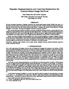
pared to the noise term σ, which means that the prior dominates over the likelihood ˆ and vice versa. The term and the estimate is close to the prior term (in this case β) pooling factor is plotted in Fig. 3.2 for a sample uniform grid input distribution centered around the origin. Here C is given by eq. (3.3), parameters h and σ were chosen arbitrarily and the local model is centered around the origin. From the plot, it is obvious that the pooling factor approaches 0 near the center of the model and approaches 1 away from the center as is expected. Also shown in the plot are the pooling factors for different values of the bandwidth h. For smaller bandwidths the curve is sharp at the bottom and is more flat for higher values of the bandwidths. This implies that for higher bandwidths the extent of data around the center of the model pooled towards the mean regression coefficient is higher and in turn leads to an increased expanse of linearity.

3.2

Locally weighted linear model

A Randomly Varying Coefficient model can also be understood as a local linear regressor. The local regression equivalent to RVC can be obtained by marginalizing out the hidden variables βi of the local model to obtain : ˆ σ, h1 . . . hd+1 ) = R P(yi |βT xi , σ2 )P(β |β, ˆ Ci )dβ P(yi |β, i i i T ⇒ yi ∼ N (βˆ xi , xTi Ci xi + σ2 )

(3.6)


31

1 0.9 σ2 = 100

0.8

pooling factor

0.7

h=1

0.6 0.5 0.4 0.3 h=10

0.2 0.1 0 −10

−8

−6

−4

−2

0 x

2

4

6

8

10

Figure 3.2: The pooling factor as a function of the input distribution

It is interesting to note that the form of likelihood in eq. (3.6) corresponds to a linear regression with heteroscedastic noise (Gelman et al., 2003). Thus the Randomly Varying Coefficient formulation strives to model the data points as being generated from a linear function with a noise process that increases monotonically with the distance from the center of the local model. This brings the model in line with the kind of heteroscedastic model we had discussed in the context of product of experts regression in Chapter 2. Assuming IID data, the log likelihood for the entire data is given by the sum of the log likelihood of individual data points defined in eq. (3.6), and can be written as : T 1 (yi − βˆ xi )2 1 T 2 L = ∑ − ln (xi Ci xi + σ ) − 2 2 (xTi Ci xi + σ2 ) i

(3.7)

Eq. (3.7) can be rewritten in a more generic form by replacing the variance part xTi Ci xi + σ2 by a weighting function

1 φ(xi ,h)

1 2

to yield : 1 2

T

L = ∑ ln φ(xi , h) − φ(xi , h)(yi − βˆ xi )2 i

(3.8)

The log likelihood L can be seen to be made up of two terms - a weighted squared error term that represents the bias of the fit and the normalization term that corresponds to the variance. The weighting function contributes to both these terms with the bandwidth parameter h of the weighting function modulating the bias and variance of the fit. The


32

optimal bandwidth would hence be a trade-off between the bias and variance and would typically depend on the functional form of the objective function being optimized.

3.2.1

The weight function for the local linear regression

As we saw in eq. (3.8), the marginal likelihood can be understood as a weighted least square regression with appropriate regularization. The nature of the weighting is governed by the weighting function that is used to provide locality. The weighting function in our model is given by φ(xi , h) = 1/(xTi Ci xi + σ2 ). This weighting function corresponds to an inverse of a quartic polynomial in x. This type of weight function has not been used previously in local least squares regression or kernel regression. Researchers usually prefer to use weight functions like Gaussian, Epanechnikov or tricubic kernels (Härdle, 1994; Loader, 1999a). However it has been noted (Härdle, 1994; Atkeson et al., 1997) that given an optimal bandwidth for a kernel the fit is not sensitive to the shape of the kernel. Hence, in this work we have chosen an inverse polynomial keeping an eye on the ease of inference afforded by this form of kernel. In this section we had formulated RVC as a local linear regression with parameters ˆ and the for the fit and bandwidth. A straightforward approach to estimate the fit (β) bandwidth (h) parameters of RVC would be to optimize the log likelihood given by eq. (3.8). However, it is observed that the maximum likelihood (ML) estimate for the fit obtained using the log likelihood suffers from substantial bias at points of high curvature along the function being modeled and requires a regularizer prior over the bandwidth parameter as explained next.

3.2.2

Bias reduction for linear fit

The log likelihood function L given by eq. (3.8) is a typical loss function for a locally weighted regression and it is generally observed that when a localised linear regression is used to obtain a smoothed estimate of a non linear function, substantial bias is introduced at points of high curvature. This is usually referred to as “trimming the hills and filling the valley” (Hastie & Loader, 1993) and is illustrated in Fig. 3.3. The phenomenon can be demonstrated by estimating the bias for a simple noiseless function defined over a one dimensional input. The log likelihood of a local model of RVC as


33

defined by eq. (3.8) can be adapted to a univariate target function as : 1 2

1 2

L = ∑ ln φ(xi , h) − φ(xi , h)( f (xi ) − m(xi − xc ) − c)2 i

where f (x) is the function to be approximated, xc the center of the local model, m the slope and c the intercept of the univariate regression. To estimate the value of the bias introduced by an ML estimate of the parameters, the slope and intercept of the weighted regression needs to be computed by differentiating L with respect to the parameters and equating to zero : ∂L = φ(xi , h)(xi − xc )( f (xi ) − m(xi − xc ) − c) = 0 ∂m ∑ i ∂L = φ(xi , h)( f (xi ) − m(xi − xc ) − c) = 0 ∂c ∑ i

(3.9) (3.10)

Solving the above simultaneous equations in m and c we obtain : ( f (xc ) − c) = f 00 (xc )

∑i φ(xi , h)(xi − xc ) ∑i φ(xi , h)(xi − xc )3 − (∑i φ(xi , h)(xi − xc )2 )2 (∑i φ(xi , h)(xi − xc ))2 − ∑i φ(xi , h) ∑i φ(xi , h)(xi − xc )2

= w f 00 (xc )

(3.11)

where f (xi ) has been replaced by its Taylor expansion about xc upto the second degree. Eq. (3.11) clearly illustrates the bias ( f (xc ) − c) as a function of the curvature represented here by the second order differential f 00 (xc ). Different methods have been proposed in the literature to reduce this bias • Using a higher degree polynomial fit can overcome the effect of higher degrees of the function. In the above derivation we have effectively shown that a linear fit can overcome bias effects of first degree, similarly a quadratic fit can overcome effects of second degree and so on. This has been proved for any generic local polynomial fit in (Hastie & Loader, 1993), (Fan & Gijbels, 1995). • As illustrated in (Choi & Hall, 1998) the bias at a point of high curvature can also be reduced by using local models in neighboring regions placed in such a way as to cancel out the effects of the bias. • If we assume that the fit is sufficiently local so that φ(x, h) has a fast decay, then the data distribution around the center of the local region can be assumed to be fairly symmetric. In addition when φ(x, h) is symmetric around xc and always


34

f(xc) Bias

c

xc

Figure 3.3: Bias for a local linear regression

nonnegative, the summation of terms of odd degree in eq. (3.11) reduces to zero. Hence, w in eq. (3.11) can be approximated as : w≈

∑i φ(xi , h)(xi − xc )2 ∑i φ(xi , h)

(3.12)

which means that in order to reduce the bias one can favor a weighting function φ(xi , h) with a small bandwidth value such that terms away from the center (large values of (xi − xc )2 ) receive a significantly low weight leading to smaller values for w. All the above methods tend to decrease the bias at the expense of an increased variance. In this work we use the last method wherein small bandwidths for local models are encouraged by using a Gamma 2 regularizer prior over the bandwidth parameters given by : h2j ∼ Gamma(a j , b j )

(3.13)

The parameter h being a scale parameter of the Normal distribution over the hidden variables βi , the Gamma distribution over h would be a conjugate to the Normal distribution and will serve to simplify inference procedure. We shall further assign noninformative Normal prior N (µ, S) for the parameter βˆ and a noninformative inverse Gamma3 prior with hyperparameters c and d for σ. We use values of µ = 0, S = 103 ×I, 2 Gamma(θ|a, b) ∼ ba θa−1 e(−bθ) Γ(a) 3 Inv − Gamma(θ|a, b) ∼ ba θ−(a+1) e(−b/θ) Γ(a)


35

Figure 3.4: The ‘local’ regression model

c = 10−3 and d = 10−3 to make the corresponding priors non-informative. We assume a uniform prior for the regularizer hyperparameters a j and b j . Fig. 3.4 summarizes the resultant probabilistic model for a single local model.

3.3

Combining the models for prediction

In the last section, we had concerned ourselves with the building of a probabilistic model for an individual local model. In this section, we look at how these local models can be combined together to form the complete model by using the product of experts regression model discussed previously in Chapter 2. In this section, we assume that the parameters of the models have been inferred and the learnt models need to be combined during prediction. Using the product of experts combination given by eq. (2.2), we get : y∼

∏ j N ( f j , 1/φ j ) Z

(3.14)

T Here, the local function f j is modeled using a linear fit : f j (x∗ ) = βˆ j (x∗ − x j ) from

eq. (3.8), x∗ is the test query point and x j is the center of the jth local model. The product of Gaussians is just another Gaussian and hence eq. (3.14) reduces to : T ∑ j φ j (x∗ )βˆ j (x∗ − x j ) , 1/ ∑ φ j (x∗ )) y |x ∼ N ( ∗ ∑ j φ j (x ) j ∗

∗

(3.15)


36

We now examine the predictive process by modeling the combined prediction as a linear smoother. Maximizing the likelihood given by eq. (3.8) with respect to the fit βˆ leads to a weighted regression solution. Writing down the maximum likelihood estimate of βˆ we get : βˆ j = (XTj W j X j )−1 XTj W j y

(3.16)

where, X = [x1 . . . xi . . . xN ]T , W j is a diagonal matrix with the diagonal elements given by W j (i, i) = φ j ((xi − x j ), h) and y = [y1 . . . yi . . . yN ]T . We can rewrite eq. (3.16) as βˆ = S j y. Substituting this form in eq. (3.15) we get the mean prediction as : j

T ∑ j φ j (x∗ )βˆ j (x∗ − x j ) E(y ) = ∑ j φ j (x∗ ) ∑ j φ j (x∗ )(x∗ − x j )T S j = y ∑ j φ j (x∗ ) ∗

= s(x∗ )T y where, s(x∗ ) =

∑ j φ j (x∗ )STj (x∗ −x j ) . ∑ j φ j (x∗ )

(3.17)

From eq. (3.17) we can conclude that the RVC model

is a linear smoother (Hastie & Tibshirani., 1990; Loader, 1999a), predicting the response to a new query point as a smooth over the target points y. The weight vector s(x∗ ) is usually called the weight function (Silverman, 1984) or the weight diagram (Loader, 1999a). It must be noted that the weight function s is a function of the design points and is completely independent of the response variable. For a fixed design with input data being regularly spaced within an interval, Silverman compares the weight function to a kernel and calls it an equivalent kernel (Silverman, 1984; Sollich & Williams, 2005). The equivalent kernel can be used to deduce the properties of the smoother as it indicates the weight received by each of the response points in accordance with its position in space. For the weight function defined in eq. (3.17), the equivalent kernel is plotted in Fig. 3.5 for three different test points with the train points being equally spaced along the input dimension.

3.3.1

Degrees of freedom

One of the ways to compare different linear smoothers is by measuring the degree of smoothness of the curve it models. The smoothness is often measured in terms of the degrees of freedom of the fit. The degrees of the freedom is also an indicator of the complexity of the learning model (in the sense of Occam’s razor) and loosely corresponds to the number of parameters used by the model. The degrees of freedom


37

0.08 0.07 0.06

equivalent kernel weight

0.05 0.04 0.03 0.02 0.01 0 −0.01 −0.02

−9.05

−5

0.05 x

5

9.05

Figure 3.5: The weights produced by the equivalent kernel at different test points for a uniformly spaced train points.

of a smoother can be computed by looking at the trace of the hat matrix (Hastie & Loader, 1993). The hat matrix is defined as the matrix that maps the responses to the fits produced by the model. We can derive the hat matrix for RVC by starting with the local model. For a local model the fit is linear and hence the hat matrix Sˆ is given by Sˆ j = X j S j = X j (XTj W j X j )−1 XTj W j such that yˆ j = Sˆ j y where yˆ j is the vector of predictions obtained from the jth local model corresponding to the vector of training responses y. The combined estimate produced by RVC is a convex combination of the estimates of different local models : yˆ =

∑ Wˆ j yˆ j j

=

∑ Wˆ j Sˆ j y

(3.18)

j

ˆ j is a diagonal normalized weight matrix with the diagonal elements given where, W ˆ j= ˆ j (i, i) = φ j ((xi −x j ),h) which can also be expressed in terms of W j as W by W ∑ j φ j ((xi −x j ),h)

(∑ j W j )−1 W j . From eq. (3.18), the effective weighted hat matrix would be Sˆ = ˆ j Sˆ j . The degree of freedom of the RVC model according to the measure de∑j W veloped in (Hastie & Loader, 1993) would be given by the trace of the hat matrix Sˆ


38

200 200 local models 100 local models

180 160

degrees of freedom

140 120 100 80 60 40 20 0 −5 10

0

5

10 bandwidth

10

Figure 3.6: Variation of degrees of freedom with bandwidth and the number of models in RVC

given by : ˆ = trace(∑ W ˆ j Sˆ j ) d f = trace(S)

(3.19)

j

It can be easily seen that the degree of freedoms of the combined system is greater than a single local model : ˆ ≥ trace(Sˆ j )∀ j∈1...M trace(S)

(3.20)

For a local model having a linear parametrization for the function, trace(Sˆ j ) would be equal to the number of dimensions of the input d. Therefore from eq. (3.20) we find that the combined model of RVC would have atleast as many degrees of ˆ as the number of dimensions of the input. As we can see from freedom(trace(S)) eq. (3.19), the degrees of freedom of the system is governed by the weighting provided to individual hat matrix. The weighting in turn is modulated by the individual bandwidths of the model. We can then expect that the degrees of freedom would be a function of the bandwidth. The variation of the degrees of freedom with the bandwidth of the models is illustrated in Fig. 3.6. Here, local models were centered around all the input points and were assigned the same bandwidth. The value of the bandwidth was varied and the effective degrees of freedom computed and plotted. The plot shows that as we increase the bandwidth the modeling ability of the model decreases as the degrees of freedom approaches that of a simple linear regression model and as the bandwidth decreases more complex surfaces can be modeled as it captures more vari-


39

ations in the given function. The other factor that influences the degrees of freedom is the number of models in the system. In Fig. 3.6 two plots have been shown to illustrate the effect of number of local models on the degrees of freedom of the system. The plot in the dashed line shows an RVC model with as many local models as data points and the plot with solid curve stands for the degrees of freedom for a case when only half of the data points are used as centers of the local models of RVC. The interesting fact to note in the figure is that as the bandwidth decreases in the top plot the degrees of freedom tends to reach the maximum which is the number of data points whereas in the bottom curve the maximum degrees of freedom exceeds the number of models in the system (in this case 100). This shows that the combined system can reach degrees of freedom exceeding the number of models. It must be noted that the illustration here has been obtained by restricting the bandwidths to be the same for all local models, this then represents a restricted subspace of the combination of the bandwidth values possible and represents a subset of the possible degrees of freedoms.

3.4

Discussion

In this chapter we had developed a probabilistic model for local linear regression and showed its links to related research literature. Furthermore we derived the complexity of the learning model for a local component of the ensemble and extended it to the entire ensemble. We also demonstrated in Section 3.3.1, that by learning the optimal bandwidth in a data driven fashion it is possible to modulate the flexibility of the model and by dynamically allocating and deallocating models in the system it is possible to enhance or limit the complexity of the system. This would be the basis for the learning algorithm of RVC developed in succeeding chapters.

Chapter 4 Learning Learning the parameters of the Randomly Varying Coefficient model implies optimizing the joint likelihood of the variables of the model. A simple maximum likelihood estimate of the parameters would tend to produce a biased (MacKay, 1992) model which overfits the training data. An alternative would be to to learn a distribution over the parameters that gives the most probable estimate of the parameter and confidence bounds over the estimates. Use of a non-informative prior over the nuisance parameters results in a posterior that is insensitive to the specific prior used and thus avoids tuning of the hyperparameters. The posterior over the parameters can then be used to marginalize out the variables during prediction. This is equivalent to taking an average of the predictions of different models and results in a more robust prediction. In the RVC model, we have non-informative priors over the parameters βˆ and σ (refer Fig. 3.4). For the bandwidth parameter h we have an informative prior with hyperparameters a j and b j . In a true Bayesian setting a non-informative prior over the hyperparameters a and b would be used to infer its posterior. However, due to the absence of any suitable conjugate prior over a and b we resort to inferring the point estimates of the hyperparameters. ˆ h j , σ and to obtain Our objective is thus to learn the posterior over the parameters β, point estimates for the hyperparameters – a j , b j . The joint posterior is given by: ˆ σ|y, a, b, c, d, µ, S) = P(h, β,

ˆ h, σ, a, b, c, d, µ, S) P(y, β, P(y, a, b, c, d, µ, S)

(4.1)

where we have used h to denote the vector [h21 . . . h2d+1 ]T and y denotes the training data [y1 . . . yN ]T , a ≡ [a1 . . . ad+1 ]T and b ≡ [b1 . . . bd+1 ]T . However, the posterior over the parameters is rendered intractable due to the difficulty in evaluating the denominator of eq. (4.1). This necessitates the use of variational Bayesian EM to evaluate the posterior 40

Chapter 4. Learning

41

ˆ σ|y, a, b, c, d, µ, S) and learn the regularizer hyperparameters a and b. P(h, β,

4.1

Variational approximation for RVC

To learn the parameters of the model we can maximize the marginal log likelihood with respect to the parameters treating βi as the hidden variables. The marginal log likelihood is given by:

L = ln P(y|a, b, c, d, µ, S) Z

ˆ σ2 |a, b, µ, S, c, d)dβ . . . dβ dhd βdσ ˆ 2 P(y, β1 . . . βN , h, β, 1 N " Z = ln ∏ P(yi|βi, σ2)P(βi|β,ˆ h1, . . . hd+1) = ln

i

# ˆ S)P(σ2 |c, d) ∏ P(h2j |a j , b j )P(β|µ,

ˆ 2 (4.2) dβ1 . . . dβN dh1 . . . dhd+1 d βdσ

j

Using Jensen’s inequality, the objective function that lower bounds L for a distribution Q is given by:

F =

Z

ˆ 2 ˆ σ2 ) ln P(y, β1 . . . βN , h, β, σ |a, b, µ, S, c, d) dβ . . . dβ dhd βdσ ˆ 2 Q(β1 . . . βN , h, β, 1 N ˆ 2 Q(β1 . . . βN , h, β, σ ) (4.3)

ˆ σ) that makes the bound tight is given by the The optimal value for Q(β1 . . . βN , h, β, ˆ σ|y) but since this posterior is intractable, we make an joint posterior P(β . . . β , h, β, 1

N

approximation by assuming that the posterior over the variables is independent and can be expressed as : 2 ˆ σ|y) = ˆ Q(β1 . . . βN , h, β, |y) ∏ Q(βi|y) ∏ Q(h2j |y)Q(β|y)Q(σ i

j

This form of approximation is often called an ensemble variational approximation (Beal, 2003), details of which can found in Appendix A. Substituting the factorized approximation in eq. (4.3) we get: "

Fapprox = ∑ hln P(yi |βi , σ)iQβ ,Q i

i

Qβi ,Qh1 ...Qhd+1 ,Q ˆ

σ

β

+ ∑ ln P(h2j |a j , b j ) Q j

#

D E ˆ h1 . . . hd+1 ) + ln P(β | β, i 2

hj

D E ˆ S) + ln P(β|µ,

Qβˆ

D E

− ∑ ln Qβ − ∑ ln Qh j Q − ln Q ˆ hj β i Qβ i j i

+ ln P(σ2 |c, d) Q

σ2

− hln Qσ2 iQ Qβˆ

σ2

(4.4)

Chapter 4. Learning

42

where h.iQ denotes the expectation with respect to the distribution Q. The optimal values of the posterior probabilities can be computed iteratively by maximizing the functional Fapprox with respect to each individual posterior distribution keeping the other distributions fixed akin to an EM procedure. The posteriors for the parameters of RVC can be derived following the same procedure detailed above. Here, we give the resulting updates for the hyperparameters of the posterior with the detailed derivation listed in Appendix B. ˆ • The update of the posterior Q(βi |y) ∼ N (νi , Gi ) keeping Q(β|y), Q(h2j |y) and Q(σ2 |y) fixed is :

Gi = (xi xTi / σ2 + hCi i−1 )−1 = hCi i −

hCi i xi xTi hCi i hσ2 i + xTi hCi i xi

by Sherman-Morrison Woodbury theorem (4.5)

D E Here, hCi i = diag(xTi xi / h2j

Q(h2j )

˜ c. ) and σ2 = d/ ˜ Furthermore, using results

from eq. (4.5),

νi = Gi (yi xi / σ2 + hCi i−1 µ˜ ) =

(4.6)

hCi i xi T µ ˜ + µ˜ y − x i i (hσ2 i + xTi hCi i xi )

ˆ ˜ keeping Q(β |y), Q(h2 |y) and ∼ N (˜µ, S) • The update of the posterior Q(β|y) i j Q(σ2 |y) fixed is : !−1 S˜ =

∑ hCii−1 + S−1

(4.7)

i

! µ˜ = S˜

∑ hCii−1 νi + S−1µ

(4.8)

i

The update given in eq. (4.8) can be seen to be equivalent to a weighted least squares regression by substituting the value of νi from eq. (4.6), S˜ from eq. (4.7) in eq. (4.8) and setting µ = 0 to obtain : !−1 ! T x x x y i i i µ˜ = ∑ hCi i−1 + S−1 ∑ hσ2i + xT hCii xi − hσ2i + xTi hCii xi − hCii−1 µ˜ i i i i (4.9) which at convergence would yield : µ˜ =

xi xTi ∑ hσ2i + xT hCii xi + S−1 i i

!−1

xi yi ∑ hσ2i + xT hCii xi i i

!

Chapter 4. Learning

43

and has the same form as a weighted regression estimate with the weights given

by σ2 + xTi hCi i xi . ˜ keeping Q(β |y), Q(h2 |y) • The update of the posterior Q(σ2 |y) ∼ Inv-Gamma(c, ˜ d) i j ˆ and Q(β|y) fixed is : c˜ = c + N/2 d˜ = d + ∑ (yi − νTi xi )2 + xTi Gi xi /2

(4.10) (4.11)

i

• The update of the posterior Q(h2j |y) ∼ Gamma(a˜ j , b˜ j ) keeping Q(βi |y), Q(σ2 |y) ˆ and Q(β|y) fixed is : a˜ j = a j + N/2 b˜ j = b j + ∑ (νi, j − µ˜ i, j )2 + Gi, j j + S˜ j j /(2xTi xi )

(4.12) (4.13)

i

Here, νi, j and µ˜ i, j denote the j-th element of the respective vectors and Gi, j j and S˜ j j denotes the j-th diagonal element. These updates are repeated till convergence. The regularizer hyperparameters a j and b j in eqs. (4.12) and (4.13) are obtained by maximizing the bound Fapprox given by eq. (4.4) with respect to these hyperparameters keeping the posterior distributions Q fixed. Such a method of hyperparameter estimation has been used previously in (Tipping & Lawrence, 2005) and suggested in (Beal, 2003). Considering only the terms of

Fapprox involving the hyperparameters we can define E as : E=

Z

Q(h2j |a˜ j , b˜ j ) ln P(h2j |a j , b j )dh2j

Maximizing E with respect to the hyperparameters is equivalent to minimizing the KL divergence between the distributions Q and P. Since the posterior Q and prior P share the same parametric form, KL divergence is minimized when the parameters of these distributions match. This leads to the simple update rule for the hyperparameters given by: a j = a˜ j , b j = b˜ j

(4.14)

The iterative training algorithm for each local model is concisely summarized in Algorithm 2.

Chapter 4. Learning

44

Algorithm 2 Training a local model 1: Initialize hyperparameters: Θ ≡ {µ0 , S, c, d, a, b}. 2:

Input: Batch training data X, y

3:

repeat ˜ using Θ and eq. (4.5), (4.6) and eqs. (4.7) Estimate posterior hyperparameters Θ

4:

- (4.13). Estimate values of the hyperparameters a and b of the regulariser prior using eq.

5:

(4.14). 6:

˜ until convergence of Θ

4.2

Prediction using the committee of local models

We have dealt so far with building a coherent probabilistic model for each local expert and have derived inference procedures to estimate the parameters of individual models. Given the ensemble of trained local models, in order to predict the response yq for a new query point xq , we take the normalized product of the predictive distribution of each local model as discussed in Chapter 2. The predictive distribution of each local model is given by: P(yq |y) =

Z

2 ˆ σ, h)Q(β|y)Q(σ ˆ ˆ 2 P(yq |β, |y)Q(h|y)dhd βdσ

(4.15)

ˆ σ, h) has the form given by eq. (3.6). We can further integrate out βˆ where P(yq |β, from eq. (4.15) to obtain the predictive distribution as : P(yq |y) =

Z

˜ σ, h)Q(σ2 |y)Q(h|y)dhdσ2 P(yq |˜µ, S,

(4.16)

Eq. (4.16) is a mixture of Gaussians with a common mean and different variances. Since the integral in eq. (4.16) is intractable, it is approximated using a Gaussian distribution given by N (˜µT xq , v2 ). A student-t distribution would be a better approximation for the particular integral, but we have chosen to approximate the predictive distribution by a Gaussian keeping in mind the ease of combining Gaussian distributions using a product of experts paradigm. By minimizing the KL divergence between the approximate distribution and the actual distribution, it can be shown (Appendix C) that the optimal value of v2 is xTq (S˜ + Chmode )xq + σ2mean where Chmode refers to the covariance matrix evaluated at the mode of the posterior Q(h|y) and σ2mean stands for the mean of Q(σ2 |y). The final predictive distribution for the k-th local model is: yq,k ∼ N (˜µTk xq,k , xq,k T (S˜ k +Ckhmode )xq,k + σ2mean ),

Chapter 4. Learning

45

Algorithm 3 Global prediction using local models 1: Input: Query point xq , learned parameters µ ˜ k , Ck , S˜ k and σk 2:

Initialize: sumα = 0, yq = 0

3:


4:

xq,k = xq − xc,k

5:

Calculate αk using eq. (4.18)

6:

yq = yq + αk µ˜ Tk xq,k

7:

sumα = sumα + αk

8:

end for

9:

Output: yq = yq /sumα , var = 1/sumα

where xq,k refers to the query point with the k-th center subtracted and augmented with bias. Blending the prediction of different experts by taking their product and normalizing it results in a Normal distribution given by : yq ∼ N (µ, ζ2 ) where µ =

1 ∑k αk µ˜ Tk xq,k , ζ2 = . ∑k αk ∑k αk

(4.17)

Here, µ is a sum of the means of each individual expert weighted by the confidence expressed by each expert in its own prediction αk , ζ2 is the variance and αk is the precision of each expert : αk = 1/(xTq,k (S˜ k +Ck )xq,k + σ2k ), Ck = diag{xTq,k xq,k /h2j,k }

(4.18)

The prediction routine for RVC combining the predictions of individual local models is summarized in Algorithm 3.

4.3

Empirical study of RVC

In this section, we carry our some empirical evaluations of the RVC algorithm in order to highlight the salient aspects of its formulation. In the implementation, the hyperparameters µ, S, c and d are set to values that make the corresponding priors noninformative. Values of µ = 0, S = 103 × I, c = 10−3 and d = 10−3 ensures such a condition. On the other hand the regularizer hyperparameters a and b are initialized such that it encourages small h as previously discussed in Section 3.2.2. A value of a = 1 and a sufficiently large value for b ensures such a bias. These settings are used for all the evaluations in the thesis.

Chapter 4. Learning

46 2 Data points True fn. 1.5

Linear fits

y

1

0.5

0

18

x

hslope

17.5

17

16.5

16 0

20

40

60

80

100

x

Figure 4.1: Local linear fits and ‘local’ bandwidth adaptation

4.3.1

Bandwidth adaptation and confidence measures

The bandwidth parameter plays a crucial role in determining the bias-variance tradeoff for each local model by determining the extent of each local model. Here, we illustrate the adaptation of bandwidth for each local model and the resulting global fits and confidence bounds of the RVC model. Fig. 4.1 shows the local linear fits (at selected test points) learnt by RVC using 300 noisy training data points from a function with varying spatial complexity(Vijayakumar et al., 2005). Such functions are extremely hard to learn since models with high bias tends to oversmooth the nonlinear regions while more complex models tend to fit the noise. While the local linear fits roughly correspond to the expected slope at the respective points (see Fig. 4.1 (top)), avoiding overfitting or oversmoothing, a more significant result is the adaptation of the local bandwidth. The bottom section of Fig. 4.1 plots the converged locality measure1 in terms of the local bandwidth parameter hslope , illustrating the adaptation to the local curvature. In another evaluation using the same toy function and 500 noisy training points, we compared the global fit and confidence bounds learned by RVC to Gaussian Process 1 Smooth

plots for the bandwidth were obtained by using local models centered around a dense uniform grid in input space.

Chapter 4. Learning

47 2

1.5

Data points True fn. Learnt fn. Confidence region

RVC

y

1

0.5

0

−0.5 0

20

40

60

80

100

x

(a) Fit and confidence bounds learnt by RVC 2

1.5

Data points True fn. Learnt fn. Confidence region

GP

y

1

0.5

0

−0.5 0

20

40

60

80

100

x

(b) Fit and confidence bounds learnt by GP

Figure 4.2: Comparison of fits learnt by RVC and GP

(GP) regression (Williams, 1998) – a state of the art regression technique. Fig. 4.2(a) and 4.2(b) shows the results of the comparison; it is important to note that we have deliberately avoided using training data in the input data range [55,65] and the confidence bounds (computed using eqs. (4.17) and (4.18) for RVC) nicely reflect this.This evaluation is aimed to demonstrate that RVC is able to adapt its confidence bounds based on the distribution of training data as well as a global learning algorithm like GP. This comparison does not include the fit learned in the region of sparse data, since the lack of data precludes any judgement about the true fit. This evaluation highlights the fact that RVC provides competitive (with respect to

48

800

420

780

400

760

380

740

360

720

340

700

320

680

300

660

280

640

260

620 00

1

2

3

4

5

6

Test likelihood

Fapprox

Chapter 4. Learning

240 7

log(b)

Figure 4.3: Sensitivity to initialization of the hyperparameters

the state of the art), approximate and appropriate confidence interval estimates while retaining the attractive properties of non-parametric, localised learning.

4.3.2

Sensitivity to initialization

Although the Variational Bayesian EM(VBEM) procedure of learning in RVC is not entirely parameter free, the majority of the parameters and hyperparameters (refer to Fig. 3.4), with the exception of the scale parameter of the Gamma regularizer hyperprior b, can be set using uninformative priors – we will demonstrate this empirically later on in this section. Maximum likelihood estimation of the regularizer hyperparameter b makes the convergence of the RVC relatively sensitive to its initialization. Next, we explore this effect on the final learned model and recommend a procedure to determine the optimal initialization for b. As an illustrative example, a noisy (std. deviation of 0.05) sinc function with 200 randomly distributed training points was used to train RVC. The training was repeated for different values of the scale parameter b of the regularizer Gamma prior. Fig. 4.3 plots the predictive likelihood of test data and the value of Fapprox as defined by eq. (4.4) after convergence of learning. These quantities are plotted against different initializations of b measured on a log scale. From the figure (and further extensive evaluations), it can be gleaned that while different initializations can lead to different points of

Chapter 4. Learning

49

convergence in the parameter space, the variation of the converged value of the objective function(Fapprox ) closely mimics that of the test likelihood. Hence, this objective function can be used as a reliable measure to choose a near-optimal initialization for the hyperparameter b. ˆ and noise In contrast to the scale hyperparameter b, for the parameters of fit (β) variance (σ2 ) – again refer Fig. 3.4, it is sufficient to use uninformative priors over them. This insensitivity can be illustrated via an example where the role of prior in learning the noise parameter σ is studied. An experiment was performed where the evolution of test likelihood was traced under three different settings of prior over the parameter σ. The value of σ enters into the learning updates through the expectation

statistic σ2 which in turn is determined by the updates of d˜ and c˜ in eqs. (4.10) and (4.11), and is given by :

2 d˜ d prior + ddata (4.19) σ = = c˜ c prior + cdata where ddata = ∑i (yi − νTi xi )2 + xTi Gi xi /2, cdata = N/2, c prior = c and d prior = d. Eq. (4.19) can then be rewritten as : D E

2 σ prior /cdata + σ2data /c prior

2 σ = (4.20) 1/cdata + 1/c prior D E

d prior data . It is evident from eq. (4.20) that the where σ2prior = c prior and σ2data = dcdata posterior estimate is a weighted average of the data estimate (σ2data , cdata ) and the prior (σ2prior , c prior ). The relative contribution of prior and data in determining the posterior can be modulated by adjusting the ratio of c prior to cdata . The learning behavior of RVC in terms of accuracy and convergence is studied under three different priors for σ2 : D E • Correct informative prior : In this setting, σ2prior is initialized to the true noise value used in generating the dataset and c prior /cdata = 5. This setting provides a higher weight to the prior belief. • Non-informative D prior : EIn this setting, c prior = 10−3 and d prior = 10−3 which corresponds to a σ2prior = 1 and c prior /cdata = 5 × 10−6 . This setting corresponds to a case where the prior is downweighted and allows the “data to speak” (Gelman et al., 2003). D E • Incorrect informative prior : In this setting, σ2prior is initialized with a random incorrect value and c prior /cdata = 5. This setting corresponds to a case where the prior belief is incorrect but is allowed to dominate over the data.

Chapter 4. Learning

50

500 Incorrect prior Correct prior Non−informative prior

400

Test likelihood

300 200 100 0 −100 −200 0

200

400 # epochs

600

800

Figure 4.4: Effect of prior on accuracy and convergence

The plots of test likelihood for these settings is shown in Fig. 4.4. As can be seen from the figure, a non-informative setting of the prior leads to the same likelihood as a correct prior albeit at a slower rate of convergence whereas an incorrect strong prior leads to a deterioration in accuracy accompanied with a slower convergence. This suggests that in the absence of any strong prior information about the values of the parameters, a non-informative prior serves as the best choice; indeed, these default settings can be carried over to different learning tasks without the need for extensive tuning. The resulting reduction in the number of open parameters in RVC is a significant improvement over other local linear regression methods like LWPR (Vijayakumar et al., 2005).

4.3.3

Allocation of local models

Modularity and independence of local models lets us adapt the complexity of the combined model by the addition and deletion of local models without affecting the existing learnt models. This property of RVC makes it useful as an adaptive, incremental learner that maintains the key benefits of local learning (Schaal & Atkeson, 1998; Vijayakumar et al., 2005) and will be exploited in Section 5.2, wherein local models are allocated and deallocated dynamically. There are two issues when dealing with the allocation of local models - the number and the position of these models in the input space. In a non-competitive local learning scenario, where local models cooperate only

Chapter 4. Learning

51

500

Test likelihood

0

Test likelihood 5 times Std. dev

−500

−1000

−1500 0

50

100 #local models

150

200

Figure 4.5: Illustration of the effect of number of local models on the quality of fit

at the prediction phase, the exact position and number of local models do not affect the quality of approximation(Atkeson et al., 1997; Schaal & Atkeson, 1998) as long as sufficient overlap is maintained. To illustrate this, noisy (std. deviation of 0.05) training data from a sinc function is used and accuracy of RVC is measured as a function of the number of local models used. To make the evaluation efficient, we exploit the fact that the local models are trained independently. Hence, instead of retraining RVC models with different number of local models, local models are placed at all the training data points and trained. A subset of these local models is then chosen to build an RVC for prediction. The RVC built in this manner is used to compute the test likelihood over a test dataset. This process of prediction is repeated for RVC built with a single local model, two local models and so on upto the maximum number of local models available. For each cardinality of the RVC, mean and variance of test likelihood is computed by repeating the test with different random selections of local models from the pool of trained local models. The statistics thus collected is shown in Fig. 4.5. From the figure, it is clear that after a certain point there is no significant increase in the accuracy with further addition of local models. Also, as seen from a larger variance at low number of local models and a much lower variance when using larger numbers of local models, the exact positioning of the local models is significant only when the number of local models are low, i.e., when there is not sufficient overlap between models. These results

Chapter 4. Learning

52

are indeed in line with other more extensive studies on local weighted learning(Atkeson et al., 1997).

4.4

Discussion

In this chapter we have formulated a principled variational approximation to the posterior probabilities over parameters of the model. The EM optimization procedure built on top of the variational Bayesian approximation allows us to develop efficient updates for the posterior probabilities of the parameters of the local model. The most interesting aspect of the learning rules for the local models is that they are completely independent of each other and hence avoid negative interference between them. Training local models is in itself not sufficient to make predictions for novel test points and requires a combination rule to combine the predictions of the local models. In this chapter we formulated such a combination rule based on the framework of product of experts. Furthermore, through empirical analysis of the RVC model in Section 4.3 we demonstrated the properties of the learning algorithm used in RVC. To summarise, the outcome of this chapter is a learning algorithm that has a probabilistic formulation and uses a Bayesian inference procedure to learn the posterior distributions over its parameters, from a batch of data. In the next chapter we modify this algorithm to make it online.

Chapter 5 Online learning In previous chapters, we have looked at the probabilistic formulation of RVC and derived learning rules that involved learning the posterior probabilities of the parameters using a batch update represented by eqs. (4.7)-(4.13). These updates can be rewritten in the form of online updates by exploiting the Bayesian formalism (Sato, 2001; Opper, 1998). In a batch mode of posterior evaluation, we have N

posteriorN = ∏ (likelihoodi ) × prior0 i=1

where i is an index over the data points. The same can be expressed as a set of online updates: posteriori ∝ likelihoodi × priori priori+1 = posteriori This set of updates implies that at every step of the online update the prior computed over the data seen so far is combined with the likelihood of the current data point to yield the posterior. This new posterior distribution of the parameter is then used as the prior during the next update. Based on this, we can derive the online updates for RVC that correspond to the batch results derived earlier : −1 S˜ i = (hCi i−1 + S−1 i )

(5.1)

µ˜ i = S˜ i (hCi i−1 νi + S−1 i µi )

(5.2)

a˜i, j = ai, j + 1/2 b˜ i, j = bi, j + (νi, j − µ˜ i, j )2 + Gi, j j + S˜ i, j j /(2xTi xi ) c˜i = ci + 1/2 d˜i = di + (yi − νTi xi )2 + xTi Gi xi /2 53

(5.3) (5.4) (5.5) (5.6)

Chapter 5. Online learning

54

Algorithm 4 Online updates for a local model 1: Initialize hyperparameters: Θ0 ≡ {µ0 , S0 , c0 , d0 , a0 , b0 }. 2:

repeat

3:

Input training data: xi , yi

4:

repeat ˜ i using Θi and eq. (4.5), (4.6) and eqs. Estimate posterior hyperparameters Θ

5:

(5.1) - (5.6). Estimate values of the hyperparameters a and b of the regulariser prior using

6:

eq. (4.14). until convergence of posteriors ˜i Θi+1 = Θ

7: 8: 9:

until end of training data

˜ = We repeat the above updates for a single data point {xi ,yi } till the posteriors Θ ˜ µ˜ , a, ˜ c, ˜ converge. For the (i + 1)-th point, we then use posterior Θ ˜ of i-th step (S, ˜ b, ˜ d) as the prior Θ = (S, µ, a, b, c, d); this procedure is illustrated in Algorithm 4. The prediction subroutine for the online algorithm remains the same as shown in Algorithm 3.

5.1

Complexity analysis of online updates

The time complexity of the learning algorithm is dominated by the computation of Gi in eq. (4.5). The equations that use Gi are eq. (5.4) and eq. (5.6) and these can be rewritten to avoid explicit computation of Gi . Eq. (5.4) requires only the diagonal elements of Gi which can be computed in O(d)(d is the number of dimensions of the input) since Gi ( j, j) = Ci ( j, j) − (Ci ( j, j)xi ( j))2 /(σ2 + γi ) using eq. (4.5) where γi = xTi Ci xi which can also be computed in O(d) due to the fact that Ci is diagonal. On the other hand, eq. (5.6) requires the evaluation of xTi Gi xi which in turn can be written down as: xTi Gi xi

σ2 γi = 2 σ + γi

and can also be computed in O(d). Furthermore, the matrix inverses in eq. (5.1) and eq. (5.2) can also be computed in O(d) due to the fact that Si and Ci are diagonal matrices. Therefore, the overall time complexity per online update is O(dM) where d is the number of dimensions and M the number of local models. The algorithm


55

does not require any data points to be stored and hence, has a O(M) space complexity for the sufficient statistics stored in the local models. The independence of the local models also means that the effective time complexity can be brought down to O(d) using M parallel processors. The time complexity for prediction is O(dM) including the evaluation of mean and the confidence bounds. We can see from this analysis that the algorithm is very efficient with respect to time and space (in fact it matches LWPR’s efficiency) and hence, is a strong candidate for situations which require real time and online learning.

5.2

Addition/deletion of local models

An important issue in online learning is the dynamic allocation of local models. It has been shown in Section 4.3.3 that typically only a subset of the training points needs to be used as centers of local models. Finding such an optimal subset of the training points, in a real time and independent learner is difficult and non-essential. The motivation behind this statement can be summarized as: • In an online setting, at any point in time there is only a partial knowledge of the target function. Hence, in theory, the optimal centers for the local models could shift with time as more samples are provided to the learner. This is particularly true when we have a changing input data distribution (also known as covariate shift) – a scenario which is very realistic in, for e.g., robot dynamics learning where data arrives in batches from one part of the workspace and then, another as opposed to a uniform distribution. • The optimal centers for the local models is a function of the global fit and cannot be determined locally and independent of other models. Moreover, truly incremental learning schemes discard training data after incorporating it into the learning model. Indeed, Section 4.3.3 has shown that sufficient overlap between local models is enough to ensure good global prediction. Hence, the local models are added using a simple heuristic based on the predictive likelihood for a new data point. The predictive likelihood for an unseen data point measures the capacity of the existing local models to explain the new data point. If the likelihood is less than a threshold parameter for all local models, then a new local model is added with the data point serving as the center.


56

0.7 −3

3

GP LWPR RVC

x 10

0.6 Test Error (nMse)

2

0.5

1

0.4

0

0.3 0.2 0.1 0

sinc

boston

ozone

Figure 5.1: Comparison of generalization error between RVC, GP and LWPR on sinc, boston and ozone data sets.

When two local models have sufficient overlap in the region they model, then one of them is redundant and can be pruned. The degree of overlap between two models can be estimated by looking at the input region where these two models have a significantly high confidence. If the two candidate models express confidence for a prediction above a fixed threshold then it is likely that the models have a significant overlap and one of them can then be pruned. In empirical studies though, we have found that if the addition of models is done judiciously then pruning does not play a significant part in the learning process. The addition and deletion heuristics used here are similar to the ones used in (Schaal & Atkeson, 1998).

5.3

Evaluation

In this section, we demonstrate the salient aspects of the RVC model by looking at some empirical test results, compare the accuracy and robustness against state of the art methods and evaluate its performance on some benchmark datasets. In the first experiment we compare the generalization performance of RVC against two other candidate algorithms - Gaussian Process(GP)(Williams, 1998) and Locally Weighted Projection Regression(LWPR)(Vijayakumar et al., 2005) on artificial as well


57

1

20 RVC # model LWPR # model

Test Error (nMse)

0.6 10 RVC

0.4

# models

SPGP #model

0.8

LWPR SPGP

0.2

0 0

GP

100

200 300 # data points

400

0 500

Figure 5.2: Comparison of online learning dynamics for sinc function

as real world datasets. The sinc function, air dataset described in (Bruntz et al., 1974) and the Boston housing dataset from the UCI repository were used as benchmark datasets. The dataset for the sinc function consisted of 500 training data points from the sinc function corrupted with output noise: ε ∼ N (0, 0.052 ) and a test dataset consisting of 1000 uniformly distributed test points. The air(ozone) dataset which is a three dimensional dataset with 111 data points was split into 83 training and 28 test points. The 13 dimensional Boston dataset was split into 404 training and 102 test points. The online learning methods – RVC and LWPR, were trained in epochs of repeated presentation of the training data, till convergence; LWPR required careful tuning of the distance metric initialization and learning rates to achieve the performance reported here as opposed to the uninformative priors used for RVC. The performance of GP, RVC and LWPR shown in Fig. 5.1 are statistics accumulated over 10 different traintest splits. Asymptotically, all three methods perform very well on the sinc data set, achieving nMSE of less than 0.0025. For the ozone dataset which is highly nonlinear, RVC and LWPR performs better than GP. For the Boston dataset, we find that the performance of RVC is close to that of LWPR while slightly inferior to the GP results – although this difference is statistically insignificant. In an evaluation to compare the online learning characteristics, we trained RVC, LWPR, GP and Sparse Pseudo-input Gaussian Process (SPGP) (Snelson & Ghahramani, 2006) algorithms on the sinc dataset described earlier. After each training data


58

8 6

−1 GP SPGP RVC

−2 −3 log(testing time)

log(training time)

4 2 0 −2

−4 −5 −6

−4

−7

−6 −8 0

GP SPGP RVC

100


400

500

−8 0

100

(a)


400

500

(b)

Figure 5.3: (a) Comparison of training time between RVC, GP and SPGP on sinc data set. (b) Comparison of time complexity for prediction.

point was presented to the learning system, the generalization error was evaluated using a uniform grid of 500 test data points. The RVC model was allowed only a single EM iteration for each data point to ensure a fair comparison with LWPR. The resulting error dynamics averaged over 10 train-test evaluations, is shown in Fig. 5.2. In this comparison, GP exhibits a sharply decreasing error curve which is not surprising considering that it is essentially a batch method and stores away all of the training data for prediction. When we compare RVC with LWPR, we find that RVC converges faster while using roughly the same order of local models. This can be attributed to the Bayesian learning rules of RVC that estimates the posterior over parameters rather than point estimates. Since the posterior is a product of likelihood and prior, in the event of sparse data (as in the initial stages of online learning), the prior ensures that the posterior distributions assigned to the parameters and in turn the predictions of the learner are reasonable. Also the optimization of the regularizer hyperparameters for every data point implies a faster adaptation and hence, a faster convergence. We can now compare accuracy and efficiency of RVC with that of a sparse version of GP namely SPGP. RVC is able to match the generalization performance of an SPGP using almost the same number of local models. A more significant result is seen from Fig. 5.3(a) where the time taken for training on the sinc dataset is illustrated for RVC and compared with an accurate yet slow full Gaussian Process and an approximate yet fast algorithm of SPGP. The difference between RVC and SPGP is very clear from Fig. 5.3(a) with RVC having a better scaling behaviour. The empirical results supports the theoretical prediction of a O(MN) time complexity for RVC compared to O(M 2 N)


59

100 Motorcycle data : GP 50

y

0

−50

−100

Data points Learnt fn. Confidence region

−150 0

10

20

30 x

40

50

60

(a) Fit and confidence bounds for GP 100 Motorcycle data: RVC 50

y

0

−50

−100

−150 0

Data points Learnt fn. Confidence region 10

20

30 x

40

50

60

(b) Fit and confidence bounds for RVC

Figure 5.4: Comparison of fit and confidence bounds for the motorcycle dataset learned by GP and RVC model, showing adaptation to heteroscedastic (varying) noise levels. The data consists of a sequence of accelerometer readings through time following a simulated motor-cycle crash.

for SPGP and O(N 3 ) for a full GP. The time required for the mean prediction are the same for RVC and SPGP - O(M) per test case and is much efficient than a full GP with O(N 3 ) complexity. These experiments thus demonstrate the favourable scaling characteristics of RVC when learning from data. Our next experiment aims to illustrate the ability of RVC to model heteroscedastic data (i.e., data with varying noise levels). Fig. 5.4(b) illustrates the fit and the confidence interval learnt on the motorcycle impact data (Silverman, 1984) discussed in (Rasmussen & Gharamani, 2000). Notice that the confidence interval correctly adapts to the varying amount of noise in the data as compared to the confidence interval learnt by a GP with squared exponential kernel shown in Fig. 5.4(a). This ability to model


(a)

60

(b)

Figure 5.5: (a) DLR LWR-III robot arm, (b) OpenGL/ODE based full contact simulation of DLR robot arm

non-stationary functions is another advantage of RVC’s localised learning. In the next evaluation, we demonstrate the utility of RVC in learning the inverse dynamics of a 7DOF KUKA Light-Weight Robot (LWR) arm (see Fig. 5.5(a)). Out of the seven degrees of freedom, three were controlled and the rest fixed. A batch train-test dataset consisting of 9 input dimensions and an output was generated using a faithful simulation (see Fig. 5.5(b)) of the robot arm performing a pseudo-randomly drifting figure-8 pattern. The input dimensions were the joint angles, velocities and accelerations whereas the output was the applied torque at the shoulder joint. A set of 1000 training and test points were used to evaluate the normalized mean square error (nMSE) and the performance averaged over 5 repeats of the evaluation. The performance of RVC compared against GP and LWPR is shown in Fig. 5.6(inset table). As can be seen from the table, for data from one of the representative joints of the robot arm, RVC and LWPR have similar performance and is significantly better than a simple linear regressor whereas GP has the best performance. This difference can be attributed to the fact that while GP utilizes the whole of the training set for prediction, RVC and LWPR is more efficient and uses only a few parameters for prediction. Finally, we used the robot arm as mentioned in the previous experiment to track a figure-8 pattern. A composite control consisting of a combination of feedforward and low gain feedback commands was used to control the joints of the arm. The feedforward command in turn was produced from an inverse dynamics model of the robot arm learnt online by an RVC model. The aim of the experiment was to learn an accurate model for the inverse dynamics of the robot arm. The RVC model was trained on data that was collected while the robot arm performed a drifting 8 pattern. The training data consisted of 2000 data points corresponding to a 8 pattern in the x-z plane and a slowly drifting y


61

0.5

z displacement

0.4 0.3

Methods

0.2

Linear

1.4 × 10−2 (±6.13 × 10−4 )

0.1

GP

1.45 × 10−7 (±8.09 × 10−9 )

RVC

1.8 × 10−3 (±2.19 × 10−4 )

LWPR

1.1 × 10−3 (±3.63 × 10−5 )

0

Trajdes Traj50

−0.1

Traj200000

Test error (nMse)

Trajpd

−0.2 −0.4

−0.3

−0.2

−0.1 0 x displacement

0.1

0.2

0.3

Figure 5.6: Progress of online learning with RVC control - Traj des is the desired trajectory, Traj 50 , Traj 200000 are the trajectories learnt from 50 and 20, 0000 training data points and Traj pd is the trajectory corresponding to a low gain PD control without any feedforward component; (table) Comparison of test errors for different learning methods.

coordinate. The training was stopped at certain intervals and the robot arm with the composite control was used to track the figure-8 pattern on a fixed x-z plane. The result of the experiment is shown in Fig. 5.6 where the pattern performed by the robot is shown at different stages of learning. As can be seen from the figure, RVC model is able to achieve a significant improvement over a simple Proportional-Derivative (PD) controller within a single pass of the training data, but requires more learning iterations to accurately track the desired trajectory. In this experiment we have compared the performance of the composite control based tracking to the PD controller to illustrate the suitability of an online learner like RVC for such control applications.

5.4

Automatic relevance determination in high dimensional input space

One of the impediments of localised learning is that, with increasing dimensions of the input space, learning the locality becomes difficult and requires a dense sampling of data in the input space. As explained and empirically demonstrated in (Vijayakumar et al., 2005; Hoffmann et al., 2009), the usual methods of dimensionality reduction like PCA is insufficient to handle this problem since PCA takes into account only the correlation amongst the input variables and ignores the information provided by the


62

0.45 Gaussian prior ARD prior

0.4 0.35

Test error (nMse)

0.3 0.25 0.2 0.15 0.1 0.05 0 0

5

10

15 20 25 Epochs of EM iteration

30

35

40

Figure 5.7: Comparison of the convergence of learning using a Gaussian prior and an ARD prior on a high dimensional dataset

response variable when determining the optimal low dimensional representation of the input space. The dimensionality reduction is more effective if the response variable is also included in the dimensionality reduction process. Consequently in this section we look at a method to reduce the dimensionality of the input space using a Automatic Relevance prior. It must be noted that while using Automatic Relevance prior allows us to choose the features it does not create new features like a PCA and so is less powerful, yet from the empirical evaluations performed later in this section we find that feature selection greatly improves the rate of convergence of the learning algorithm. The main advantage of having a Bayesian formulation for learning is that we can integrate our prior belief into the model by changing the prior distribution over parameters. When we need to handle large number of input dimensions with some of them being irrelevant, it is efficient to identify and eliminate the irrelevant dimensions. It is especially useful to have an automatic relevance determination in RVC because of its use of distance measures defined on the input space to measure the locality of a model. When we eliminate the irrelevant bandwidth parameters from the model, the learning becomes more efficient. We can achieve an automatic relevance determination by using a sparsity encouraging prior similar to (Figueiredo, 2003). In the original model illustrated in Fig. 3.4, we change the prior over the regression coefficient βˆ from a zero mean Gaussian to a zero mean Laplacian distribution leading to ˆ ˆ 1) P(β|α) ∝ exp(−αkβk


63

ˆ 1 denotes the l1 norm and α is the scale parameter of the Laplace distriwhere kβk ˆ However the bution. We can use this prior to find the posterior distribution over β. Laplace prior is not a conjugate distribution of the Gaussian distribution and requires approximation inorder to evaluate the posterior. We approximate the posterior over βˆ by a Gaussian distribution using a Laplace approximation. In our case the log posterior over βˆ is given by : D E ˆ ˆ M = ln Q(β|y) ∝ ln P(βi |β, Ci )

Q(βi ),Q(h)

ˆ + ln P(β|α)

(5.7)

Laplace approximation of the posterior corresponds to ˆ ∼ N (˜µ, S) ˜ Q(β|y) is the Hessian of the negative log where µ˜ = argmax ˆ M and S˜ −1 = −∇∇M | ˆ β=˜µ β posterior. The posterior mode µ˜ can be obtained by setting the gradient of M to zero and when C is diagonal we can evaluate the value of µ for each dimension separately: α µ˜ j = sgn(v j ) |v j | − (5.8) ∑i 1/Ci ( j, j) + where sgn(.) is the sign of the argument, (.)+ is defined as 0 when the argument is less −1 −1 than 0 else it takes the value of the argument itself, v = ∑i Ci ∑i µi C−1 i and j is the index over the dimensions. The variance of the posterior is given by the Hessian which is defined as -

 −1 −1  µ˜ 6= 0 ∑i Ci S˜ =  unde f ined otherwise

(5.9)

When any component of the vector µ˜ goes to zero we prune that particular dimension from the training data and from the model. This makes the learning very efficient. To demonstrate the effectiveness of the sparsity prior in determining irrelevant variables, we use a 5 dimensional sinc dataset with 4 of its dimensions being irrelevant. We run the RVC algorithm with an ordinary Gaussian prior and compare it with a Laplacian ARD prior with α set to a value of 0.1. It must be noted that there exist a number of methods to learn the value of α (Figueiredo, 2003), but here we have used the value of α that gave the maximum value for the training likelihood with multiple restarts. The evolution of the test error with each epoch of the EM is shown in Fig. 5.7. We find that the algorithm with the ARD prior is able to converge faster by pruning the irrelevant dimensions. In the final experiment we demonstrate the ability of RVC with an ARD prior to learn in high dimensions with many irrelevant input dimensions in the data. RVC is


64

1.4 SPGP RVC 1.2

Test error (nMse)

1

0.8

0.6

0.4

0.2

0

5d

10d

20d

Figure 5.8: Performance of SPGP and RVC on datasets of increasing dimensions. Shown on the plot are the mean and a single standard deviation of 10 train-test splits of data with 500 train and test points.

run on a sinc dataset with 5, 10 and 20 dimensions out of which only one dimension is relevant. The test error of RVC is compared against SPGP in Fig. 5.8. The SPGP algorithm was run using the matlab implementation of sparse GP with default settings and using as many local models as the RVC. The result demonstrates that RVC is able to match up with SPGP in terms of its generalization ability. It must be noted that SPGP did not use an ARD prior since the results obtained for the ARD priors were worse than that of an ordinary RBF prior and requires careful initialization of parameters before training to obtain better generalization performance (Snelson & Ghahramani, 2006).

5.5

Discussion

In the initial part of this chapter we modified the training updates of RVC to enable learning from data in an online manner. This process was simplified due to the use of Bayesian inference procedure that naturally yields online updates. In the second half of the chapter we provided extensive empirical evaluations to highlight the different strengths of the RVC formulation Generalization ability : Generalization ability of RVC was compared against other learning algorithms on well known multivariate benchmark datasets in Fig. 5.1 and was found to be fairly competitive compared to the other learning algorithms.


65

Online learning dynamics : RVC was shown to have a favourable online learning and fairly fast convergence as compared to related learning algorithms in Fig. 5.2. Efficiency : RVC has a very efficient learning and prediction routines as compared to learning algorithms like GP and was demonstrated in Fig. 5.3. Heteroscedastic noise : The ability to model heteroscedastic noise is another of the positives of RVC and is shown in Fig. 5.4. Scalability : The RVC model scales up well with increasing number of data points learning them online. This is illustrated in experiments with the robot arm shown in Fig. 5.6 and it also scales up well with increasing number of input dimensions as shown in Fig. 5.8. From these evaluations it can be seen that while RVC is well suited for a high dimensional data rich environment which requires fast learning with limited space complexity.

Chapter 6 Classification using Randomly Varying Coefficient model In this chapter we look at a different scenario of learning where we are concerned with classifying given data points into different classes. The essential difference between a regression as we have been examining in the previous chapters, and classification lies in the nature of the response variable. In regression the response is continuous valued while in classification the response has discrete values corresponding to the discrete classes. While in regression we aim to approximate the mapping between the input and the response, in classification the aim is to discriminate between the classes conditional on the input. Research in classification has been dominated by kernel based methods like Support Vector Machine (SVM)(Vapnik, 1998) and more recently by non-parametric methods like Gaussian Process Classification (GP)(Rasmussen & Williams, 2006). Non-parametric methods like GP derives its success by using a covariance function of the input to model the dependency amongst the responses. The response for a test input is then computed as a linear smooth of all the training responses. This in turn leads to a large overhead in the time and space complexities for training and prediction. The training time complexity for GP is O(N 3 ) for a data of size N and O(N 2 ) for prediction. For an SVM, the training time complexity for an active set of size M in the worst case is O(MN 2 ). These are significant overheads for large datasets. There have been many sparse Gaussian Process formulations (Csatò & Opper, 2002; Williams & Seeger, 2001; Smola & Bartlett, 2001; Tresp, 2000) that try to reduce this overhead but the efficiency still is quadratic in the size of the active set for most of these implementations. When we deal with online classifiers the space complexity also becomes an overarching concern. As seen in previous chapters Ran66

Chapter 6. Classification using Randomly Varying Coefficient model

67

domly Varying Coefficient (RVC) model exhibits a good generalization performance at a low cost - O(MN). Hence, we can use RVC to learn decision boundaries that would discriminate between classes.

6.1

Local logistic regression

We modify the RVC designed originally for regression into a classifier by using a logistic link function to convert a continuous response produced by a regressor into a value that lies between 0 and 1. This value in turn can be interpreted as the probability of the data belonging to a particular class. For a binary class variable zi , the probability that zi = 1 is modeled as the output of a logistic link function over a continuous latent variable yi expressed as : p(zi = 1|yi ) = 1/(1 + exp(−yi )) In turn, the latent variable yi is modelled as the response of a locally linear regression. For a locally linear region centered around xc a conditional model for the continuous latent variable yi is modelled as in eq. (3.1) and can be written as: yi = βTi xi + ε

(6.1)

where xi ≡ [(x0i − xc )T , 1]T represents the center subtracted, bias augmented input (1)

(d+1) T ]

vector, βi ≡ [βi . . . βi

represents the corresponding regression coefficient and

ε ∼ N (0, σ2 ) is the Gaussian mean zero noise with a variance σ2 . We follow the same formulation of RVC given in eq. (3.2) and define βi as : ˆ Ci ) βi ∼ N (β,

(6.2)

with Ci being a diagonal matrix given by : Ci ( j, j) = xTi xi /h2j where h j is the bandwidth of the jth dimension. By marginalizing the hidden variables βi we end up with a model for the local linear regression as : T yi ∼ N (βˆ xi , xTi Ci xi + σ2 )

(6.3)

Proceeding along the same lines as Chapter 3 of (Rasmussen & Williams, 2006) and Section 5.3 of (Gelman & Hill, 2007) we now assume a noise-free latent variable yi by setting σ2 to zero. Setting σ2 to zero yields the following model for yi : yi ∼ N (βTi xi , 0)


68

Figure 6.1: Probabilistic model of the logistic regressor

or equivalently marginalizing yi : p(zi = 1|βi ) = 1/(1 + exp(−βTi xi ))

(6.4)

which corresponds to the classical formulation of a linear logistic regression with regression coefficients βi . We preserve the same probabilistic model as the original RVC for the rest of parameters. This includes a Gamma regularizer prior over the bandwidth parameters : h2j ∼ Gamma(a j , b j )

(6.5)

ˆ We assume a uniform and a noninformative Normal prior N (µ, S) for the parameter β. prior for the regularizer hyperparameters a j and b j . The resultant probabilistic model for a single local model of the logistic regressor is shown in Fig. 6.1. Next, we infer the posterior distribution over the parameters of the model using Bayesian inference rules.

6.2

Learning the parameters

ˆ h j is given by: The joint posterior over the parameters β, ˆ a, b, µ, S) = P(h, β|z,

ˆ h, a, b, µ, S) P(z, β, P(z, a, b, µ, S)

(6.6)

where we have used h to denote the vector [h21 . . . h2d+1 ]T and z denotes the training data [z1 . . . zN ]T , a ≡ [a1 . . . ad+1 ]T and b ≡ [b1 . . . bd+1 ]T . However, the posterior over the


69

parameters is rendered intractable due to the difficulty in evaluating the denominator of eq. (6.6). This necessitates the use of variational Bayesian EM to evaluate the posterior ˆ a, b, µ, S) similar to Chapter 4 and learn the regularizer hyperparameters a and P(h, β|z, b. To learn the parameters of the model we can maximize the marginal log likelihood with respect to the parameters treating βi as hidden variables. The marginal log likelihood is given by:

L = ln P(z|a, b, µ, S) Z

ˆ b, µ, S)dβ . . . dβ dhd βˆ P(z, β1 . . . βN , h, β|a, 1 N

Z

ˆ S)dβ . . . dβ dh1 . . . dhd+1 d βˆ ∏ P(zi|βi)P(βi|β,ˆ h1, . . . hd+1) ∏ P(h2j |a j , b j )P(β|µ, 1 N

= ln = ln

j

i

Using Jensen’s inequality, the objective function that lower bounds L for a distribution Q is given by:

F =

Z

ˆ ˆ ln P(z, β1 . . . βN , h, β|a, b, µ, S, c, d) dβ . . . dβ dhd βˆ (6.7) Q(β1 . . . βN , h, β) 1 N ˆ Q(β1 . . . βN , h, β)

ˆ that makes the bound tight is given by the joint The optimal value for Q(β1 . . . βN , h, β) ˆ but since this posterior is intractable, we make a factorized posterior P(β . . . β , h, β|z) 1

N

approximation by assuming that the posterior over the variables is independent and can be expressed as : ˆ = ˆ Q(β1 . . . βN , h, β) ∏ Q(βi|z) ∏ Q(h2j |z)Q(β|z) i

j

Substituting the factorized approximation in eq. (6.7) we get: D E ˆ h1 . . . hd+1 ) Fapprox = ∑ hln P(zi |βi )iQβ + ln P(βi |β,


i

i

β

+ ∑ ln P(h2j |a j , b j ) Q

hj

j

D E ˆ + ln P(β|µ, S)

(6.8)

Qβˆ

− ∑ ln Qh j Q − ln Q ˆ hj β Q Qβi j

D E − ∑ ln Qβ i

i

βˆ

where h.iQ denotes the expectation with respect to the distribution Q. The optimal values of the posterior probabilities can be computed iteratively by maximizing the functional Fapprox with respect to each individual posterior distribution keeping the other distributions fixed akin to EM. For a logistic regression, an additional complication arises in the computation of the posterior distribution over the hidden variables


70

βi . The likelihood term P(zi |βi ) is given by the logistic link function whereas the prior over βi is Gaussian and is not conjugate to the likelihood term. We solve this issue by using a Laplacian approximation to approximate the posterior over βi by a Gaussian distribution.

6.2.1

Laplace approximation of Q(βi |z)

Frequently in Bayesian inference of complicated probabilistic models that employs non-conjugate priors, the posterior is approximated by a Gaussian distribution centered around the mode of the actual posterior. This is usually termed as the Laplace approximation (Tierney & Kadane, 1986). In our case the log posterior over the hidden variable βi is given by : D

E

ˆ Ci ) M = ln Q(βi |z) = ln P(zi |βi ) + ln P(βi |β, − ln

Z

ˆ ),Q(h) Q(β E D ˆ Ci ) exp(ln P(zi |βi ) + ln P(βi |β, ˆ ),Q(h) ) Q(β

(6.9)

Laplace approximation of the posterior corresponds to Q(βi |z) ∼ N (νi , Gi ) where νi = argmaxβi M and G−1 i = −∇∇M |βi =νi is the Hessian of the negative log posterior. The posterior mode νi can be obtained by setting the gradient of M to zero. However, this procedure does not yield a closed form solution for the posterior mode νi . We then have to resort to Newton’s update to find the mode iteratively as shown : −1 νi = νold i − (∇∇M ) ∇M

(6.10)

ˆ Ci ) and P(zi |β ) from eqs. (6.2) and (6.4) into eq. (6.9) Substituting the forms of P(βi |β, i and differentiating it with respect to βi we get : ∇M |β =νold = xi (zi − πi ) − hCi i−1 (νold ˜) i −µ

(6.11)

∇∇M |β =νold = −xi xTi πi (1 − πi ) − hCi i−1

(6.12)

i

i

i

where πi =

i

1/(1 + exp(−xTi νold i ))

D E and hCi i = diag(1/ h2j

Q(h2j ) −1

T from eq. (6.12) that G−1 i = −∇∇M = xi xi πi (1 − πi ) + hCi i

). It can be found

and the estimate for νi

can be obtained by substituting eqs. (6.11) and (6.12) in eq. (6.10) yielding : −1 old νi = νold ˜ )) i + Gi (xi (zi − πi ) − hCi i (νi − µ


71

which can be simplified using Sherman-Morrison Woodbury theorem to yield :

where wi =

6.2.2

hCi i xi xTi hCi i wi + xTi hCi i xi hCi i xi T ˜ ) + µ˜ = ((zi − πi )wi + xTi νold i − xi µ T (wi + xi hCi i xi )

Gi = hCi i −

(6.13)

νi

(6.14)

1 πi (1−πi ) .

ˆ and Q(h2 |z) Posteriors for Q(β|z) j

Posterior over βˆ based on the likelihood and the prior over βˆ can be derived as : ˆ ∼ N (˜µ, S) ˜ Q(β|z) where S˜ = (∑ hCi i−1 + S−1 )−1

(6.15)

˜ ∑ hCi i−1 νi + S−1 µ) µ˜ = S(

(6.16)

i

i

Similarly, the posterior over h j is given by : Q(h2j |z) ∼ Gamma(a˜ j , b˜ j ) where a˜ j = a j + N/2 b˜ j = b j + ∑ (νi, j − µ˜ i, j )2 + Gi, j j + S˜ j j /2xTi xi

(6.17) (6.18)

i

where νi, j and µ˜ i, j represent the jth element of the vectors. The regularizer hyperparameters a j and b j in eqs. (6.17) and (6.18) are obtained by maximizing the bound

Fapprox given by eq. (6.8) with respect to these hyperparameters keeping the posterior distributions Q fixed. This leads to the same update rule as eq. (4.14) for the hyperparameters and is given by: a j = a˜ j , b j = b˜ j

(6.19)

The posterior parameters are inferred by using a partial Newton step to infer the posterior of βi followed by EM updates. The procedure for training a local model is summarised in Algorithm 5.


72

Algorithm 5 Training a local model 1: Initialize hyperparameters: Θ ≡ {µ0 , S, a, b}. 2:

Input: Batch training data X, z

3:

repeat 1 Initialize νold ˜ , πi = 1/(1 + exp(−xTi νold i =µ i )) and wi = πi (1−πi ) . ˜ using Θ and eq. (6.13), (6.14) and eqs. Estimate posterior hyperparameters Θ

4: 5:

(6.15) - (6.18). Estimate values of the hyperparameters a and b of the regularizer prior using

6:

eq. (6.19). 7:

˜ until convergence of Θ

6.3

Prediction

Using the learning procedure discussed in the previous section we obtain independently trained local models of the logistic regression. Each of the local models represent a separate classifier with a linear decision boundary. To obtain an aggregate prediction for a particular query input we need to combine the classifiers. Ensemble learning has been a field of research which has seen considerable amount of research into the ways of combining classifiers (Kittler et al., 1998). In this thesis though we use the same technique as RVC - combining the linear regressors to produce a non-linear regression model and then using a logistic transform to obtain a classifier. Given the ensemble of trained local experts, in order to predict the response yq for a new query point xq , we take the normalized product of the predictive distribution of each local expert. This results in the predictive distribution for the k-th local model : yq,k ∼ N (˜µT xq,k , xq,k T (S˜ k + Ckhmode )xq,k ) where xq,k refers to the query point with the k-th center subtracted and augmented with bias. Blending the prediction of different experts by taking their product and normalizing it results in a Normal distribution given by: yq ∼ N (µ, ζ2 ) where µ =

1 ∑k αk µ˜ Tk xq,k , ζ2 = . ∑k αk ∑k αk

(6.20)

Here, µ is a sum of the means of each individual expert weighted by the confidence expressed by each expert in its own prediction αk , ζ2 is the variance and αk is the precision of each expert: αk = 1/(xTq,k (S˜ k + Ck )xq,k )

(6.21)


73

Algorithm 6 Global prediction using local models 1: Input: Query point xq 2:

Initialize: sumα = 0, yq = 0

3:


4:

xq,k = xq − xc,k

5:

Calculate αk using eq. (6.21)

6:

yq = yq + αk µ˜ Tk xq,k

7:

sumα = sumα + αk

8:

end for

9:

yq = yq /sumα

10:

Output : P(zq = 1) = 1/(1 + exp(−yq )) The predictive probability for the logistic regression can be obtained by combining

the predictive probability of the latent variable yq with the link function and marginalizing the latent variable to yield : Z

P(zq = 1|z) =

P(zq = 1|yq )P(yq |z)dyq

(6.22)

where P(zq = 1|yq ) is a logistic function and P(yq |z) is the predictive distribution given by eq. (6.20). The integral given in eq. (6.22) cannot be evaluated analytically and we must rely on numerical methods or sampling to evaluate the integral. In the context of binary classification if we threshold the predictive probability at

1 2

in order to discrimi-

nate between classes a MAP prediction would be the same as an averaged prediction as shown in (Bishop, 1995) and explained in (Rasmussen & Williams, 2006). Therefore we use MAP predictive estimate for classification. To obtain the MAP prediction we evaluate the integral in eq. (6.22) by approximating P(yq |z) by a delta function at its mode. The prediction routine is listed in Algorithm 6.

6.4

Evaluation

In the first evaluation, we look at the ability of logistic RVC (lRVC) to discriminate between two classes on a one dimensional artificial data. The data used in the task has previously been used in (Rasmussen & Williams, 2006) and is shown in Fig. 6.2. The data consists of two classes distributed such that there is linear separability at one region (between cluster centered at -6 and cluster centered at 0) and there is no clear separation in the other region (cluster centered at 0 and cluster centered at 2). This


74

1

predictive probability

0.8 0.6

0.4 0.2

0 −8

Class 0 Class 1 lRVC GP −6

−4

−2

0

2

4

6

x

Figure 6.2: Comparison of the decision boundary learnt by lRVC and GP

data was used to train lRVC with local models placed at all the training points and a Laplacian GP classifier with a square exponential covariance function. The predictive probability curve learnt by the two classifiers is compared in Fig. 6.2. It is interesting to observe that the predictive probabilities assigned by lRVC to the data points lying in the inseparable region is less than the probabilities assigned to the separable part of the class. The local modeling of lRVC ensures that the decision boundaries learnt by the local models is based on the local spatial distribution of the class and hence in this case is more confident about the linearly separable part of the input space than the non-separable data. On the other hand, GP assigns almost the same and sometimes more (Rasmussen & Williams, 2006) predictive probability to the inseparable points than the separable ones which is not very intuitive for a classifier. Before we proceed to detailed evaluation experiments, we need to specify the evaluation measures that would be used to compare different classifiers. We compare classifiers based on two different measures - misclassification error and target information. The former is the often used loss function that measures the mean number of misclassifications produced by a classifier on a test set. The target information criteria refers to a loss function that takes into account the confidence expressed by the classifier about


75

its prediction. The loss function is given by : # " 1 q q log2 (P(zi = 1|xi )) + ∑ log2 (1 − P(zi = 1|xi )) + 1 I= N z∑ zi =0 i =1 and it measures in bits, the information conveyed by the classifier about the test target. For a baseline classifier that assigns classes at random I → 0 and for a more confident discrimination of classes I → 1.

6.4.1

Comparison of generalization performance and time efficiency

In the next evaluation, we compare the generalization performance of lRVC against a Gaussian Process classifier and a baseline probabilistic linear logistic regressor. The lRVC used in the evaluation used around 20 local models initialized at the cluster centers in the input space. The Gaussian Process uses a square exponential kernel and a logistic link function. The three classifiers are compared on different benchmark datasets listed in Table 6.1. The Breast cancer, Heart (Cleveland) and the Ionosphere dataset were obtained from the UCI repository, Pima and synthetic datasets are the same as the ones used in (Ripley, 1996) 1 . The USPS dataset corresponds to the digit discrimination task listed in (Rasmussen & Williams, 2006). The Catalysis and Gatineau datasets were obtained from the predictive uncertainty challenge 2 were the validation set has been used as test set. The evaluations on the datasets obtained from UCI was carried out on 10 train-test splits of the data and the mean and standard deviations are reported here. For all other datasets a single train-test trial was carried out using the train and test files provided. This makes it possible to compare other classifiers that have previously used the latter datasets. For the Gatineau dataset GP was trained using a subset of 1000 training points due to practical considerations of time and space complexity. The evaluation statistics are listed in Table 6.2. Also shown in the table is the results for a LIBSVM(Chang & Lin, 2001) (with an RBF kernel) evaluation over the same datasets. The comparison for SVM is restricted to the misclassification error since SVM does not provide a predictive probability. One can see from the results that lRVC is able to match the performance of GP for all the datasets and outperforms the baseline linear classifier especially when the target information is used for the comparison. It must be noted that while lRVC used only a small number of local models for prediction, GP used all of the training set for training and prediction. To emphasize this difference Table 6.3 shows the time taken by lRVC and GP for training and prediction on a dataset 1 The

datasets can be obtained from http://www.stats.ox.ac.uk/pub/PRNN/

2 http://predict.kyb.tuebingen.mpg.de/pages/home.php


Dataset

#train pts. #test pts #dim

Breast cancer

142

427

30

Heart(Cleveland) 149

148

13

Ionosphere

175

176

33

Pima

200

332

7

Synthetic

250

1000

2

USPS(3-5)

767

773

256

Catalysis

873

300

617

Gatineau

3000

2176

1092

76

Table 6.1: Statistics of the benchmark datasets

lRVC

GP

Linear

SVM

Error

Information

Error

Information

Error

Information

Error

Breast

0.028(0.007)

0.807(0.010)

0.026(0.009)

0.805(0.045)

0.042(0.014)

0.797(0.050)

0.028(0.009)

Heart

0.166(0.017)

0.432(0.049)

0.169(0.017)

0.423(0.039)

0.173(0.024)

0.388(0.113)

0.173(0.022)

Ionosphere

0.152(0.027)

0.338(0.170)

0.123(0.025)

0.535(0.054)

0.163(0.027)

-2.288(0.963)

0.078(0.025)

Pima

0.202

0.361

0.222

0.276

0.198

0.364

0.198

Synthetic

0.100

0.649

0.093

0.658

0.114

0.611

0.100

USPS(3-5)

0.045

0.798

0.025

0.794

0.040

0.476

0.023

Catalysis

0.303

0.143

0.303

0.150

0.343

-3.516

0.323

Gatineau

0.090

0.570

0.090

0.588

0.154

-0.484

0.090

Table 6.2: Performance comparison between lRVC and GP in terms of the misclassification error rate and the target information (measured in bits) conveyed by the classifier. The values in parenthesis indicate the standard deviation.

consisting of the USPS digit 3 classified against the rest of the digits. lRVC can be seen to achieve a good generalization performance with a low overhead.

6.4.2

Rejection using the predictive confidence bounds

In the last evaluation, we evaluate the confidence bounds learnt by lRVC by plotting the relation between the reject rate, the misclassification error and the target information. In this experiment the first and second moments for the predictive probability were computed by using sampling to evaluate the integral in eq. (6.22). The test samples which had a variance above a threshold were rejected and the misclassification error was evaluated for the rest of the test data. The dataset used for this purpose was the

Chapter 6. Classification using Randomly Varying Coefficient model Method

GP

lRVC

77

0

1

2

4

5

6

7

8

Error

0.0108

0.0028

0.0183

0.0046

0.0259

0

0.0024

0.0254

9 0.0061

Information

0.8944

0.9027

0.8627

0.8686

0.7943

0.8857

0.8677

0.8550

0.8486

Train time(sec)

1915.9

1475.8

1020.8

877.0

911.4

963.7

919.9

845.8

993.0

Test time(sec)

47.8

37.6

25.0

22.1

20.2

23.8

23.4

20.5

24.4

Error

0.009

0.005

0.022

0.005

0.045

0.003

0.009

0.032

0.012

Information

0.944

0.960

0.886

0.966

0.798

0.972

0.955

0.883

0.946

Train time(sec)

582.59

509.67

440.44

402.23

382.08

400.75

370.25

363.13

383.42

Test time(sec)

0.87

0.74

0.61

0.61

0.55

0.55

0.54

0.49

0.55

Table 6.3: Comparison between the time taken for training and prediction by lRVC and

0.05

1

0.04

0.8 lRVC GP Linear

lRVC GP Linear

0.03

0.6

0.02

0.4

0.01

0.2

0 0

0.2

0.4 0.6 reject rate

0.8

test information, bits

misclassification rate

GP on the USPS dataset.

0 1

Figure 6.3: Comparison of error-reject curve for lRVC and GP

USPS data. The misclassification error typically decreases as test samples are rejected and an ideal classifier would have a larger reduction in the misclassification error with respect to the rejection rate. The error and the target information versus the rejection rate for lRVC, GP and the Bayesian linear logistic regressor were evaluated and plotted in Fig. 6.3. It can be seen that lRVC’s performance exceeds that of the linear classifier by a large margin and is not significantly different from GP.

6.4.3

Dynamics of online learning

Similar to Chapter 5 we can derive the online updates for the batch updates. The online updates for the logistic RVC are the same as eqs. (5.1) - (5.4) derived in Chapter


1

20 RVC GP

18 RVC # model

0.8

16 14

0.6

12 10

0.4

8

# models

Misclassification error

78

6 0.2

4 2

0 0

50


200

0 250

Figure 6.4: Online learning dynamics of lRVC compared with GP. The plots are the average performance over 10 trials of different orders of data presentations.

5. In the last evaluation, we use these online updates to learn a classifier on the synthetic dataset. The data points are presented to the online learner one at a time and the misclassification error is evaluated over the test data after each training update. The dynamics of the learning process is shown in Fig. 6.4. The learning dynamics is compared with the generalization performance of GP which uses increasing number of training data points and the corresponding test error at each stage is displayed. It can be seen from the figure that online version of lRVC exhibits fast convergence and matches the performance of GP asymptotically.

6.5

Discussion

In this chapter we extended the learning framework of RVC from a regression setting to handle classification. We used a logistic link function to turn regression into classification. From the evaluations in this chapter we can see that local logistic regression is a very competitive method. The result makes it more significant when we take it into account that the logistic regression is able to achieve such a good performance using a small number of local models. Moreover the time and space efficiency is linear in terms of the data points and the dimension. In contrast, kernel classification paradigms like GP and SVM have a much higher overhead in training and testing.


79

The use of variational Bayesian EM approximation for learning the parameters of the model allows us to reformulate the learning rules into a set of online updates for the parameters that would enable the logistic classifier to learn from data in real time. The logistic regression formulation in this thesis is restricted to binary classification. It can be easily extended to a multi-class classification using a softmax link function instead of a logistic link function. The treatment of the learning remains the same in that case too. In conclusion, the contribution of this chapter has been a probabilistic formulation of a local linear logistic regressor that can learn online using very efficient Bayesian updates and at the same time exhibits good learning characteristics.

Chapter 7 Contributions and future work The major contribution of the thesis is the development of a Bayesian formulation for independent spatially localised learners for multivariate nonlinear regression. We have used a novel formulation of data dependent priors in order to carve out locally linear regions while avoiding competition amongst local models. The ‘non-competitive’ behavior of each local model allows independent, efficient learning while the Bayesian regularizer hyperpriors guard against the danger of overfitting or over-smoothing through automatic local bandwidth adaptation. In this chapter we summarize the contributions made in this thesis along with future avenues of research possible. In this thesis, use of a product of regression experts explained in Chapter 2 has been shown to be a feasible approach to follow when we require efficient learners that can learn in an online manner and dynamically adjust model complexity. Furthermore in this thesis we have derived the connection between the ambiguity formulation of regression ensembles and a product of regression experts in eq. (2.5). Another novelty is the use of POE to bridge the gap between previously unrelated pieces of research - conditional random fields, independent ensemble learning and complementary prior. Though it is difficult to assimilate independent ensemble learning into a probabilistic framework, it is useful in designing efficient learning systems. Therefore it is worthwhile to compare the framework of dependent learning to that of independent learning by treating the latter as an approximation to the dependent learning. In eq. (2.10) we provide a bound that characterizes the error between an independent and a dependent learning. In future this bound could be further refined to quantify the effect of independent learning on the generalization ability of a learning algorithm. Chapter 3 provides a unique probabilistic formulation of a locally weighted learning using a heteroscedastic variance component to weight the errors. This type of a 80

Chapter 7. Contributions and future work

81

model has not been used for locally weighted learning, nonetheless, eq. (3.8) demonstrates the equivalence of heteroscedastic model to a locally weighted regression. Section 3.3.1 examines the ability of RVC to adapt its model complexity and illustrates the change in the complexity of the learning model through a plot of the varying degrees of freedom in Fig. 3.6. The plot provided in Fig. 3.6 is a result of an empirical analysis of the degrees of freedom; it might be possible to extend this to a more analytical treatment wherein we can derive a closed form functional relation between the degrees of freedom of RVC and the bandwidths of individual local models. Chapter 4 provides a simple Variational Bayesian EM procedure to train the local models efficiently. These learning updates are very efficient with each EM update being O(MN) where M is the number of local models and N the number of training points. Furthermore, Bayesian inference procedure also yields a predictive distribution with a mean prediction and a confidence bound on the prediction. The predictive distribution of RVC is shown to provide meaningful confidence bounds through an illustrative example in Fig. 4.2. The Variational Bayesian algorithm provides efficient updates but the approximation itself tends to have a slow convergence rate. One of the possible avenues of future research will be to use algorithms like (Qi & Jaakkola, 2006) to speed up the convergence of the VBEM algorithm. In Chapter 5 we derived the online updates for the Variational Bayesian EM learning and evaluated the RVC model against the state of the art in non-linear regression techniques on artificial as well as real world data sets. RVC matched the generalization performance of LWPR while avoiding cumbersome parameter tuning for initialization (refer Fig. 5.1, Fig. 5.2). It achieves competitive performance compared to GP - essentially a batch method, while being much more computationally efficient (refer Fig. 5.3). One of the main advantages of spatially localised models of RVC is its ability to model locally constant but globally varying properties of a function like heteroscedastic noise. The ability of RVC to model heteroscedastic noise is illustrated in Fig. 5.4 where it is compared with a GP on a benchmark dataset and is shown to perform better than a GP. The RVC is also shown to scale well with increasing dimensions of the input space in Section 5.4 where an ARD prior is used to learn in a high dimensional space with lots of irrelevant dimensions and its performance is compared with other learning methods in Fig. 5.8. In Fig. 5.6 we also demonstrate a practical application of RVC in learning the inverse model of robotic arm and is shown to perform well compared to other similar methods. The pros and cons of RVC compared against other learning algorithms have been compared in Table 7.1. The space and computational efficiency of RVC

Chapter 7. Contributions and future work

82

coupled with the ability to grow model complexity in a data driven fashion makes it a strong candidate for practical online and real time learning scenarios and was the basis for (Edakunni et al., 2007) The probabilistic formulation of RVC can further be exploited to extend it to generalized linear models and has been illustrated in Chapter 6 by formulating a logistic regression based on the model of RVC. The classifier based on RVC was also evaluated against the state of the art methods and was found to exhibit good generalization properties with a low computational complexity as illustrated by Tables 6.2 and 6.3. This work formed the basis for (Edakunni & Vijayakumar, 2009). Active learning is another area of research that can be pursued in the context of the work presented in this thesis. While traditional research has concentrated on active learning in global models of learning, the localised independent models of RVC provide an alternative strategy for active learning. The active learning itself can be localised with the learning of the fit and the number of models being learnt actively. This effort is aided by the presence of a probabilistic confidence bound provided by each of the local models constituting the ensemble. To conclude, this thesis presents an online, spatially localised ensemble learning method with efficient Bayesian inference rules that provides competitive generalization results for a variety of learning scenarios.

O(M 2 N) per gradient de-

O(N 3 ) per gradient descent

Large

Large

Number of open parameters

Projected regression

O(M)

Small

None

ARD prior

O(N 2 )

Small

Few open parameters

Scales poorly on ARD prior

O(MN)

number of training data points.

Table 7.1: Comparison of the features of the learning algorithms discussed in this thesis. Note that here, M is the number of models and N the

convergence on training

Number of data points for

informative prior

non-

All parameters other than

Open parameters have

ARD prior

Handling high dimensions bandwidth

O(M)

Space complexity

tion

O(M)

O(M) per data point

rameters

rameters

tion

MAP estimate of hyperpa-

MAP estimate of hyperpa-

Yes

Leave-one-out cross valida-

Yes

No

O(M)

O(M) per data point

Time complexity for trainO(M)

Variational Bayesian EM

Training method

No

No

No

Time complexity for predic-

Yes

Probabilistic framework

Yes

No

Yes

scent step

Yes

IID assumption for data

Yes

Yes

SPGP

O(N 2 )

Yes

Online

Yes

GP

step

Yes

Non-parametric

LWPR

ing

RVC

Features

Chapter 7. Contributions and future work 83

Appendix A Variational Bayesian Expectation Maximization In this section we introduce the variational Bayesian expectation maximization algorithm as applied to a generic graphical model involving hidden variables and distributions over those variables. We start with a simple model with the visible data given by D which stands for the collection of training data of N points whose ith individual point is represented by Di . The hidden variable associated with each individual data point is given by the variable zi . The likelihood is given by P(D|z1 . . . zN ). Assuming that the data is conditionally independent the likelihood can be written down as : N

P(D|z1 . . . zN ) = ∏ P(Di |zi )

(A.1)

i=1

The hidden variables are assumed to have been generated from a distribution given by : P(z1 . . . zN |θ) where θ is the parameter of the prior distribution. The prior distribution over the hidden variables is assumed to be conditionally independent : P(z1 . . . zN |θ) = ∏ P(zi |θ)

(A.2)

i=N

and the prior over the parameter θ is given by P(θ|α) where α is the hyperparameter. We are now interested in inferring the posterior distribution over the parameter θ. Following Bayes’ rule, the posterior is given by : P(θ|D) =

P(D|θ)P(θ|α) P(D|α)

(A.3)

Here, P(D|θ) is obtained by integrating over the hidden variables from the joint distribution : Z

P(D|θ) =

P(D|z1 . . . zN )P(z1 . . . zN |θ)dz1 . . . dzN 84

(A.4)

Appendix A. Variational Bayesian Expectation Maximization

85

The integration in eq. (A.4) leads to a closed form expression for P(D|θ) only when P(z1 . . . zN |θ) is conjugate to P(D|z1 . . . zN ). We assume from hereon that the distribution is conjugate. The prior over the parameter P(θ|α) is also assumed to be conjugate to P(z1 . . . zN |θ). Despite these pairwise conjugate distributions the posterior over the parameter θ is rendered intractable due to the difficulty in evaluating the evidence term P(D|α) in the expression in eq. (A.3). The cause of this problem is the integration involved in evaluating the evidence term : Z

P(D|α) =

P(D|θ)P(θ|α)dθ

and this would lead to a closed form expression only when P(θ|α) is conjugate to P(D|θ) which is generally not the case. In order to infer the posterior over the parameters we can start with the marginalized likelihood given by : Z

P(D, α) =

P(D|z)P(z|θ)P(θ|α)dzdθ

(A.5)

where z ≡ [z1 . . . zN ]. Taking the log of the likelihood given in eq. (A.5) we get :

L = ln P(D|α) = ln

Z


Using Jensen’s inequality L can be lower bounded by F given by :

L = ln ≥

Z


Z

Q(z, θ) ln

P(D|z)P(z|θ)P(θ|α) dzdθ Q(z, θ)

= F

(A.6) (A.7) (A.8)

where Q(z, θ) is any arbitrary function of z and θ that integrates to unity. The inequality of eq. (A.7) becomes an equality when Q(z, θ) equals the joint posterior of the random variables. But as we had seen earlier this distribution is intractable and our aim is to estimate this posterior distribution. We can constrain the form of the joint posterior as a factorized form of distribution which implies Q(z, θ) ≈ Q(z)Q(θ). Substituting this factorized form in eq. (A.7) we get : P(D|z)P(z|θ)P(θ|α) dzdθ (A.9) Q(z)Q(θ) can be seen to be a functional form of the distributions Q(z) and Q(θ)

F ≈ Fapprox =

Here, Fapprox

Z

Q(z)Q(θ) ln

and we can maximize Fapprox iteratively with respect to the free distributions. These iterative steps would essentially form the updates for the Variational Bayesian EM (VBEM) algorithm.


A.1

86

VBE step

In the VBE step we try to estimate the posterior distribution over the hidden variables Q(z) and is obtained by taking the functional derivative of Fapprox defined by eq. (A.9) with respect to Q(z) and equating it to zero : Z R ∂Fapprox ∂ Q(z) ln P(D, z|θ, α)dz = Q(θ)dθ ∂Q(z) ∂Q(z) Z

=

[ln P(D, z|θ, α) − ln Q(z) − 1] Q(θ)dθ

= 0

(A.10) (A.11) (A.12)

Solving for Q(z) we get : Z

ln P(D, z|θ, α)Q(θ)dθ

ln Q(z) ∝

(A.13)

Substituting the form of P(D, z|θ, α) from eq. (A.1) and (A.2) we get : Z N

∑ ln [P(Di|zi)P(zi|θ)]Q(θ)dθ

ln Q(z) ∝ ⇒ ∑ ln Q(zi ) ∝

i=1 Z N

∑ ln [P(Di|zi)P(zi|θ)]Q(θ)dθ

i

i=1

Z

ln [P(Di |zi )P(zi |θ)]Q(θ)dθ

(A.14)

Taking exponential of both sides of eq. (A.14) we get : Q(zi ) ∝ exp (ln P(Di |zi )) exp hln P(zi |θ)iQ(θ)

(A.15)

⇒ ln Q(zi ) ∝

where h.iQ denotes the expectation with respect to the distribution Q. When P(zi |θ) belongs to the exponential family of distribution the term hln P(zi |θ)iQ(θ) results in a distribution belonging to the same family and as a result the posterior over the hidden variable Q(zi ) is given by : ˆ Q(zi ) ∝ P(Di |zi )P(zi |θ) ˆ where P(zi |θ) = exp hln P(zi |θ)iQ(θ) is a distribution conjugate to P(Di |zi ). This leads to a closed form expression for the distribution of the posterior Q(zi ). We can see that the end result of the VBE step is an approximate posterior for the hidden variable. In the next step of the procedure we use this approximate posterior over the hidden variable to estimate the posterior over the parameter θ.


A.2

87

VBM step

In this step we estimate the posterior over the parameter assuming that the estimate of the posterior over the hidden variable is known and is equal to the current estimate from the VBE step. We use the same strategy as before to obtain the estimate of the posterior. We take the functional derivative of Fapprox with respect to Q(θ) and equate it to zero to obtain : ∂Fapprox = ∂Q(θ)

R hR

∂

i ln P(D, z|θ) + ln P(θ|α Q(θ) Q(θ)dθ ∂Q(θ)

Z

=

ln P(D, z|θ)Q(z)dz + ln P(θ|α − ln Q(θ) + c

= 0 Solving for the equation we get : ln Q(θ) ∝ ln P(θ|α) + hln P(D, z|θ)iQ(z)

(A.16)

Applying exponential on both sides and using eq. (A.1) and (A.2), eq. (A.16) becomes : *  +

∑ ln P(Di, zi|θ)

Q(θ) ∝ exp 

i

P(θ|α) Q(zi )

! ∝ exp

∑ hln P(Di, zi|θ)iQ(zi)

P(θ|α)

i

∝

hln exp P( D , z |θ)i i i ∏ Q(zi ) i

We can make the same arguments as for the VBE step and show that if the distributions involved belong to the conjugate exponential family, the posterior over the parameter has a closed form expression and belongs to the exponential family as well. The two steps of VBE and VBM are repeated iteratively till convergence. Furthermore, it can be proven that this procedure is guaranteed to minimize the KL divergence between the actual joint posterior distribution P(z, θ|D) and the approximate posterior distribution Q(z)Q(θ).

Appendix B Derivation of VBEM posteriors for RVC We start with the approximate lower bound of the loglikelihood given by : " D E ˆ hln P(yi |β , σ)i + ln P(β |β, h1 . . . hd+1 ) Fapprox =

∑

i

i

Qβi ,Qσ2

i


β

+ ∑ ln P(h2j |a j , b j ) Q

hj

j

D E ˆ S) + ln P(β|µ,

Qβˆ

− ∑ ln Qβi Q − ∑ ln Qh j Q i

#

βi

hj

j

E D − ln Qβˆ

+ ln P(σ2 |c, d) Q

Qβˆ

σ2

− hln Qσ2 iQ

σ2

(B.1)

B.1

Derivation of Qβi

The form for the posterior over βi can be derived by performing a functional differentiation of Fapprox with respect to Qβi and equating it to zero. This would yield : D E ∂Fapprox ˆ hln = P(y |β , σ)i + ln P(β | β, h) − ln Z − ln Qβi = 0 (B.2) i i i Q 2 ∂Q βi

Qh ,Qβˆ

σ

D E ˆ h) ⇒ ln Qβi = hln P(yi |βi , σ)iQ 2 + ln P(βi |β, σ

Qh ,Qβˆ

− ln Z

(B.3)

where Z is the normalization term for the posterior probability. Expanding eq. (B.3) by taking the expectations with respect to the posteriors of the other parameters we get :

1 1 ln Qβi ∝ − (yi − βTi xi )2 1/σ2 − (βi − µ˜ )T hCi i−1 (βi − µ˜ ) 2 2 ⇒ Qβi ∼ N (νi , Gi ) with 1 T Gi = (xi xi + hCi i−1 )−1 σ2 1 + hCi i−1 µ˜ ) νi = Gi (yi xi σ2 88

Appendix B. Derivation of VBEM posteriors for RVC

D E where, hCi i = diag(xTi xi / h2j

Q(h2j )

B.2

) and

D E 1 σ2

89

= c/ ˜ d.˜

Derivation of Qσ2

Performing a functional differentiation of Fapprox with respect to Qσ2 and equating it to zero would yield : ∂Fapprox ∂Qσ2

= ∑i hln P(yi |βi , σ)iQβ + ln P(σ2 |c, d) − ln Z − ln Qσ2 = 0

(B.4)

i

⇒ ln Qσ2 = ∑i hln P(yi |βi , σ)iQβ + ln P(σ2 |c, d) − ln Z

(B.5)

i

Taking expectations and expanding eq. (B.5) yields : 1 1 1 T 2 T 2 2 2 ln Qσ2 ∝ ∑ − ln σ − (yi − νi xi ) /σ − xi Gi xi /σ − (c + 1) ln σ2 − d/σ2 2 2 2 i ˜ with ⇒ Qσ2 ∼ I G (c, ˜ d) c˜ = c + N/2 d˜ = d + ∑ (yi − νTi xi )2 + xTi Gi xi /2 i

B.3

Derivation of Qβˆ

Equating to the zero, the functional differential of Fapprox with respect to Qβˆ yields : D E ∂Fapprox ˆ ˆ (B.6) ∂Qβˆ = ∑i ln P(βi |β, Ci ) Q ,Q + ln P(β|µ, S) − ln Z − ln Qβˆ = 0 βi h D E ˆ S) − ln Z ˆ Ci ) ⇒ ln Qβˆ = ∑i ln P(βi |β, + ln P(β|µ, (B.7) Qβi ,Qh

Taking expectations and expanding eq. (B.7) yields : 1 1 −1 T ˆ ˆ ln Qβˆ ∝ ∑ − (βi − β) hCi i (βi − β) − (βˆ − µ)T S−1 (βˆ − µ) 2 2 i ˜ with ⇒ Q ˆ ∼ N (˜µ, S) β

S˜ = (∑ hCi i−1 + S−1 )−1 i

˜ ∑ hCi i−1 νi + S−1 µ) µ˜ = S( i

B.4

Derivation of Qh j

The diagonal structure of Ci ensures that the posterior over Qh factorizes into individual components Qh j . Performing a functional differentiation of Fapprox with respect to

Appendix B. Derivation of VBEM posteriors for RVC

Qh j and equating it to zero would yield : D E ∂Fapprox ˆ = ln P(β | β, C ) + ln P(h2j |a j , b j ) − ln Z − ln Qh j = 0 ∑i i i ∂Qh j Qβi ,Qβˆ D E ˆ Ci ) ⇒ ln Qh j = ∑i ln P(βi |β, + ln P(h2j |a j , b j ) − ln Z Qβi ,Qβˆ

90

(B.8) (B.9)

Taking expectations and expanding eq. (B.9) yields : # " 2 +G ˜ jj (ν − µ ˜ ) + S 1 1 i, j i, j j i, j h2j + (a j − 1) ln h2j − b j h2j ln Qh j ∝ ∑ ln h2j − Tx 2 2 x i i i ⇒ Qh j ∼ G (a˜ j , b˜ j ) with a˜ j = a j + N/2 b˜ j = b j + ∑ (νi, j − µ˜ i, j )2 + Gi, j j + S˜ j j /(2xTi xi ) i

Appendix C Approximation of predictive distribution We approximate predictive distribution given in eq. (4.16) by P(yq |˜µT xq , v) where, P(yq |˜µT xq , v) ∼ N (˜µT xq , v2 ) The KL divergence between the two distributions is given by, R Z Z P(yq |˜µ, σ, h)Q(h|y)Q(σ|y)dhdσ P(yq |˜µ, σ, h)Q(h|y)Q(σ|y)dhdσ ln dyq P(yq |˜µT xq , v) (C.1) where, ˜ q + σ2 ) P(yq |˜µ, σ, h) ∼ N (˜µT xq , xTq (Ch + S)x

(C.2)

We need to optimise eq. (C.1) with respect to v. Writing down the term dependent on v and exchanging the order of integration we get, Z Z T L =− P(yq |˜µ, σ, h) ln P(yq |˜µ xq , v)dyq Q(h|y)Q(σ|y)dhdσ Z T =− P(yq |˜µ, σ, h) ln P(yq |˜µ xq , v)dyq

(C.3)

Q(h|y),Q(σ|y)

˜ q + σ2 xTq (hCh iQ(h|y) + S)x 1 1 Q(σ|y) = ln v2 + 2 2 2 v where, hCh iQ(h|y) = diag(xqT xq

2 σ Q(σ|y) =

1 h2j

Gamma(h2j )

2 σ InvGamma(σ2 ) =

) = Chmode σ2mean

˜ q +σ2mean . Differentiating L w.r.t to v and equating to zero we get v2 = xTq (Chmode + S)x 91

Bibliography Akaike, H. (1974). A new look at the statistical model identification. IEEE Transactions on Automatic Control, 19, 716–723. Allen, D. M. (1974). The relationship between variable selection and data augmentation and a method of prediction. Technometrics, 16, 125–127. Atkeson, C., Moore, A., & Schaal, S. (1997). Locally weighted learning. Artificial Intelligence Review, 11, 76–113. Beal, M. J. (2003). Variational algorithms for approximate Bayesian inference. Doctoral dissertation, Gatsby Computational Neuroscience Unit, University College London. Bishop, C. M. (1995). Neural networks for pattern recognition. Claredon Press. Bishop, C. M., & Svensèn, M. (2003). Bayesian hierarchical mixture of experts. Uncertainty in Artificial Intelligence. Brown, G., Wyatt, J., Harris, R., & Yao, X. (2005a). Diversity creation methods: A survey and categorisation. Journal of Information Fusion, 6, 5–20. Brown, G., Wyatt, J. L., & Tino, P. (2005b). Managing diversity in regression ensembles. Journal of Machine Learning Research, 6, 1621–1650. Bruntz, S. M., Cleveland, W. S., Kleiner, B., & Warner, J. L. (1974). The dependence of ambient ozone on solar radiation, temperature and mixing height. Symp. Atmospheric Diffusion and Air pollution. MIT Press. Chang, C.-C., & Lin, C.-J. (2001). LIBSVM: a library for support vector machines. Software available at http://www.csie.ntu.edu.tw/ cjlin/libsvm. Choi, E., & Hall, P. (1998). On bias reduction in local linear smoothing. Biometrika, 85, 333–345. 92

Bibliography

93

Cleveland, W. S., & Loader, C. (1995). Smoothing by local regression: Principles and methods (Technical Report). AT&T Bell Laboratories. Csatò, L., & Opper, M. (2002). Sparse on-line Gaussian processes. Neural Computation, 14, 641–668. De Forest, E. L. (1873). On some methods of interpolation applicable to the graduation of irregular series. Annual Report of the Board of Regents of the Smithsonian Institution for 1871, 275–339. De Forest, E. L. (1874). Additions to a memoir on methods of interpolation applicable to the graduation of irregular series. Annual Report of the Board of Regents of the Smithsonian Institution for 1873, 319–353. Demirekler, M., & Altinçay, H. (2002). Plurality voting-based multiple classifier systems: statistically independent with respect to dependent classifier sets. Pattern Recognition, 35, 2365–2379. Dietterich, T. G. (2002). Ensemble learning. In M. Arbib (Ed.), The handbook of brain theory and neural networks, 405–408. The MIT Press. Edakunni, N. U., Schaal, S., & Vijayakumar, S. (2007). Kernel carpentry for online regression using randomly varying coefficient model. International Joint Conference on Artificial Intelligence (pp. 762–767). Edakunni, N. U., & Vijayakumar, S. (2009). Efficient online classification using an ensemble of bayesian linear logistic regressors. Multiple Classifier Systems (pp. 102–111). Fan, J., & Gijbels, I. (1995). Adaptive order polynomial fitting: Bandwidth robustification and bias reduction. Journal of Computational and Graphical Statistics, 4, 213–227. Fan, J., & Gijbels, I. (1996). Local polynomial modelling and its applications. Chapman and Hall. Figueiredo, M. A. (2003). Adaptive sparseness for supervised learning. IEEE Transactions on Pattern Analysis and Machine Intelligence, 25, 1150–1159. Freund, Y., & Schapire, R. (1996). Game theory, online prediction and boosting. Ninth Annual Conference on Computational Learning Theory (pp. 325–332).

Bibliography

94

Gasser, T., Kneip, A., & Köhler, W. (1991). A flexible and fast method for automatic smoothing. Journal of American Statistical Association, 86, 643–652. Gelman, A., Carlin, J. B., Stern, H. S., & Rubin, D. B. (2003). Bayesian data analysis. Chapman and Hall/CRC. Second edition. Gelman, A., & Hill, J. (2007).

Data analysis using regression and multi-

level/hierarchical models. Cambridge University Press. Gelman, A., & Pardoe, I. (2006). Bayesian measures of explained variance and pooling in multilevel (hierarchical) models. Technometrics, 48, 241–251. ¨ Gram, J. P. (1883). Uber entwickelung reeller functionen in reihen mittelst der methode der kleinsten quadrate. Journal für Mathematics, 94, 41–73. Härdle, W. (1994). Applied nonparametric regression. Cambridge University Press. Hashem, S., & Schmeiser, B. (1995). Improving model accuracy using optimal linear combinations of trained neural networks. IEEE Transactions on Neural Networks, 6, 792–794. Hastie, T., & Loader, C. (1993). Local regression: Automatic kernel carpentry. Statistical Science, 8, 120–129. Hastie, T. J., & Tibshirani., R. J. (1990). Generalized additive models. Chapman and Hall. Hinton, G. E. (1999). Product of experts. Ninth International Conference on Artificial Neural Networks. Hinton, G. E., Osindero, S., & Teh, Y.-W. (2006). A fast learning algorithm for deep belief nets. Neural Computation, 18, 1527–1554. Hoffmann, H., Schaal, S., & Vijayakumar, S. (2009). Local dimensionality reduction for nonparametric regression. Neural Processing Letters, 29, 109–131. Jones, M., Marron, J., & Sheather, S. (1996). A brief survey of bandwidth selection for density estimation. Journal of the American Statistical Association, 91. Jones, M. C., Davies, S. J., & Park, B. U. (1994). Versions of kernel-type regression estimators. Journal of the American Statistical Association, 89, 825–832.

Bibliography

95

Kittler, J., Hatef, M., Duin, R. P. W., & Matas, J. (1998). On combining classifiers. IEEE Transactions on Pattern Analysis and Machine Intelligence, 20, 226–239. Krogh, A., & Vedelsby, J. (1995). Neural network ensembles, cross validation, and active learning. Advances in Neural Information Processing Systems (pp. 231–238). Kschischang, F. R., Frey, B. J., & Loeliger, H. A. (2001). Factor graphs and the sumproduct algorithm. IEEE Transactions on Information Theory, 47, 498–519. Kuncheva, L. I., & Whitaker, C. J. (2003). Measures of diversity in classifier ensembles and their relationship with ensemble accuracy. Machine Learning, 51, 181–207. Kuncheva, L. I., Whitaker, C. J., Shipp, C. A., & Duin, R. P. W. (2000). Is independence good for combining classifiers ?

International Conference on Pattern

Recognition. Lafferty, J., McCallum, A., & Pereira, F. (2001). Conditional random fields: Probabilistic models for segmenting and labeling sequence data. International Conference on Machine Learning. Loader, C. (1999a). Local regression and likelihood. Springer-Verlag. Loader, C. R. (1999b). Bandwidth selection : Classical or plug-in ? The Annals of Statistics, 27, 415–438. Longford, N. T. (1993). Random coefficient models. Clarendon Press. MacKay, D. J. C. (1992). Bayesian interpolation. Neural Computation, 4, 415–447. Mallows, C. L. (1973). Some comments on c p . Technometrics, 15, 661–675. Murray, I., & Ghahramani, Z. (2004). Bayesian learning in undirected graphical models: Approximate mcmc algorithms. Proceedings of the 20th Annual Conference on Uncertainty in Artificial Intelligence (UAI). Nadaraya, E. A. (1964). On estimating regression. Theory of Probability and its Applications, 9, 141–142. Opper, M. (1998). A Bayesian approach to on-line learning. In On-line learning in neural networks, 363–378. New York, NY, USA: Cambridge University Press.

Bibliography

96

Price, P. N., Nero, A. V., & Gelman, A. (1996). Bayesian prediction of mean indoor radon concentrations for minnesota counties. Health Physics, 71, 922–936. Qi, Y. A., & Jaakkola, T. S. (2006). Parameter expanded variational bayesian methods. Advances in Neural Information Processing Systems. MIT Press. Rasmussen, C. E., & Gharamani, Z. (2000). Infinite mixtures of Gaussian process experts. Advances in Neural Information Processing Systems 14. MIT Press. Rasmussen, C. E., & Williams, C. K. I. (2006). Gaussian processes for machine learning. MIT Press. Ripley, B. D. (1996). Pattern recognition and neural networks. Cambridge University Press. Ruppert, D., Sheather, S. J., & Wand, M. P. (1995). An effective bandwidth selector for local least squares regression. Journal of the American Statistical Association, 90. Sato, M. (2001). Online model selection based on the variational Bayes. Neural Computation, 13, 1649–1681. Schaal, S., & Atkeson, C. (1998). Constructive incremental learning from only local information. Neural Computation, 10, 2047–2084. Schapire, R. E. (1999). A brief introduction to boosting. Proceedings of the Sixteenth International Joint Conference on Artificial Intelligence. Silverman, B. W. (1984). Spline smoothing : The equivalent variable kernel method. The Annals of Statistics, 12, 898–916. Smola, A., & Bartlett, P. (2001). Sparse greedy Gaussian process regression. Advances in Neural Information Processing Systems 13 (pp. 619–625). MIT Press. Snelson, E., & Ghahramani, Z. (2006). Sparse gaussian processes using pseudo-inputs. Advances in Neural Information Processing Systems 18 (pp. 1257–1264). MIT press. Sollich, P., & Williams, C. K. I. (2005). Using the equivalent kernel to understand gaussian process regression. Advances in Neural Information Processing Systems. Spencer, J. (1904). On the graduation of the rates of sickness and mortality. Journal of the Institute of Actuaries, 38, 334–347.

Bibliography

97

Sutton, C., & McCallum, A. (2005). Piecewise training of undirected models. 21st Conference on Uncertainty in Artificial Intelligence. Szegö, G. (1992). Orthogonal polynomials. American Mathematical Society. Tierney, L., & Kadane, J. (1986). Accurate approximations for posterior moments and marginal densities. Journal of the American Statistical Association, 81. Tipping, M. E., & Lawrence, N. D. (2005). Variational inference for Student-t models: Robust Bayesian interpolation and generalised component analysis. Neurocomputing, 69, 123–141. Tresp, V. (2000). A Bayesian committee machine. Neural Computation, 12, 2719– 2741. Vapnik, V. N. (1998). Statistical learning theory. Wiley, New York. Vijayakumar, S., D’Souza, A., & Schaal, S. (2005). Incremental online learning in high dimensions. Neural Computation, 17. Vijayakumar, S., D’Souza, A., Shibata, T., Conradt, J., & Schaal, S. (2002). Statistical learning for humanoid robots. Autonomous Robot, 12, 55–69. Waterhouse, S., Mackay, D., & Robinson, T. (1996). Bayesian methods for mixture of experts. Advances in Neural Information Processing Systems (pp. 351–357). MIT Press. Watson, G. S. (1964). Smooth regression analysis. Sankhya Ser. A, 26, 359–372. Williams, C. K. I. (1998). Prediction with Gaussian processes: from linear regression to linear prediction and beyond. In M. I. Jordan (Ed.), Learning in graphical models, 599–621. Kluwer. Williams, C. K. I., & Seeger, M. (2001). Using the Nyström method to speed up kernel machines. Advances in Neural Information Processing Systems 13 (pp. 682–688). MIT Press. Woodrofe, M. (1970). On choosing a delta-sequence. Annals of Mathematical Statistics, 41, 1665–1671.

Bibliography

98

Woolhouse, W. S. B. (1870). Explanation of a new method of adjusting mortality tables, with some observations upon Mr. Makeham’s modification of Gompertz’s theory. Journal of the Institute of Actuaries, 15, 389–410. Xu, L., Hinton, G., & Jordan, M. I. (1995). An alternative model for mixtures of experts. Advances in Neural Information Processing Systems, 7, 633–640.

Bayesian Locally Weighted Online Learning

Bayesian Locally Weighted Online Learning

Suggest Documents

Learning Locally Minimax Optimal Bayesian Networks

Locally Weighted Naive Bayes - CiteSeerX

Locally Weighted Learning Model Predictive Control for ... - IEEE Xplore

Real-Time Robot Learning With Locally Weighted ... - Semantic Scholar

Optimal Bayesian Online Learning - CiteSeerX

Bayesian Nonparametric Weighted Sampling Inference

Robust Tracking with Weighted Online Structured Learning

Locally Weighted Projection Regression (LWPR) - CiteSeerX

Implementation of Locally Weighted Projection Regression Network

Face Recognition with Weighted Locally Linear ... - CiteSeerX

Locally Weighted Full Covariance Gaussian Density Estimation.

Weighted locally convex spaces of measurable functions

An approach to online Bayesian learning from

Online Bayesian Passive-Aggressive Learning - arXiv

Bayesian Online Learning on Riemannian ... - Semantic Scholar

Locally adaptive multiscale Bayesian method for ...

Bayesian hierarchically weighted finite mixture ... - Oxford Journals

Weighted Bayesian Classification based on ... - Semantic Scholar

Are Online Shoppers Interested in Learning about Locally Grown

BNFinder2: Faster Bayesian network learning and Bayesian ...

Learning Bayesian Networks

Learning Bayesian Networks - CiteSeerX

Bayesian Representations and Learning

BAYESIAN LEARNING WITH WASSERSTEIN