bayesian optimization of visual comfort - Semantic Scholar

BAYESIAN OPTIMIZATION OF VISUAL COMFORT

THÈSE NO 3918 (2007) PRÉSENTÉE LE 15 NOVEMBRE 2007 À LA FACULTÉ DE L'ENVIRONNEMENT NATUREL, ARCHITECTURAL ET CONSTRUIT LABORATOIRE D'ÉNERGIE SOLAIRE ET PHYSIQUE DU BÂTIMENT PROGRAMME DOCTORAL EN ENVIRONNEMENT

ÉCOLE POLYTECHNIQUE FÉDÉRALE DE LAUSANNE POUR L'OBTENTION DU GRADE DE DOCTEUR ÈS SCIENCES

PAR

David LINDELÖF ingénieur physicien diplômé EPF et de nationalité suédoise

acceptée sur proposition du jury: Prof. A. Mermoud, président du jury Prof. J.-L. Scartezzini, Dr N. Morel, directeurs de thèse Prof. L. Halonen, rapporteur Prof. S. Morgenthaler, rapporteur Dr T. Schumann, rapporteur

Suisse 2007

Now Faithful play the Man, speak for thy God: Fear not the wicked’s malice, nor their rod: Speak boldly man, the Truth is on thy side; Die for it, and to Life in triumph ride. John Bunyan, The Pilgrim’s Progress

Abstract We propose a self-commissioning, user-adaptive blinds and electric lighting controller for small office rooms. Self-commissioning, in this context, means that the controller builds an internal representation of the room, in particular of the room’s daylighting characteristics, automatically and without user input. By user-adaptive, we mean that the illuminances the controller will seek to maintain are derived from a statistical analysis of the user’s behaviour on the manually overridable blinds and electric lighting. Self-commission and user-adaptation are implemented by two decoupled software elements. The first element is a method for modeling the daylighting illuminance on arbitrary locations in the office room, when the windows are shaded by one or two venetian blinds (though the method can be generalized to an arbitrary number and kinds of window shadings). It uses the past history of illuminance distributions in the office room for a similar scene configuration, and models the current illuminance on a given point as a linear combination of outdoor global and diffuse irradiance. The second element is an algorithm for the estimation of the user’s visual discomfort probability. It is a function of the current illuminance distribution in that office room, and of the past history of the user’s interactions with the blinds’ and lighting controls. A bayesian formalism is applied to infer the probability that any illuminance distribution should be considered by the user as visually uncomfortable. We describe how these elements have been integrated in a blinds and electric lighting controller. That controller runs today on an office room of the experimental LESO building and we present the results of the algorithm’s adaptation to the preferences of that room’s user. We have also assessed that controller’s performance on computer-simulated virtual office rooms. We have let the controller run for one year simulated time on six different combinations of office room location (Rome and Brussels) and orientation (north, west and south). These simulations have let us evaluate the energy savings made possible with such a controller, and the improvement of the user’s visual comfort. Keywords: Bayes’s theorem, daylighting controller, user adaptation, self-commissioning, smart buildings, embedded controller, non-parametric density estimation, linear daylighting model.

i

Abstract

ii

R´ esum´ e Nous proposons un syst`eme de commande automatique de stores v´enitiens et de l’´eclairage ´electrique pour des bureaux individuels. Ce syst`eme s’adapte, d’une part, aux caract´eristiques lumineuses du bureau concern´e; et d’autre part, aux pr´ef´erences de l’utilisateur, en choisissant des niveaux d’´eclairement en fonction d’une analyse statistique du comportement de l’utilisateur sur les commandes mises `a sa disposition. Deux modules logiciels d´ecoupl´es permettent la double adaptation aux caract´eristiques du bureau et aux pr´ef´erences de l’utilisateur. Nous d´ecrivons ces deux modules qui constituent ce syst`eme de commande. Dans un premier temps nous d´ecrivons une m´ethode de pr´ediction de l’´eclairement naturel sur des points arbitraires dans un bureau, pour des fenˆetres munies d’un ou deux stores v´enitiens (la m´ethode se g´en´eralise facilement ` a un nombre arbitraire de protections solaires). La m´ethode consiste `a consid´erer l’´eclairement en un point donn´e, et pour une configuration de sc`ene donn´ee, comme une combinaison lin´eaire de l’irradiance globale et diffuse ext´erieure. Dans un deuxi`eme temps, nous d´ecrivons un algorithme pour l’estimation de la probabilit´e d’inconfort visuel de l’utilisateur. Fonction de la distribution de l’´eclairement dans la pi`ece, la m´ethode utilise le formalisme bayesien pour analyser les situations ayant par le pass´e provoqu´e une intervention manuelle de l’utilisateur sur ses stores ou l’´eclairage ´electrique. De cette analyse, une probabilit´e d’inconfort visuel peut ˆetre d´eriv´ee pour toute distribution d’´eclairement. Ces deux ´el´ements ont ´et´e int´egr´es dans un r´egulateur de stores v´enitiens et d’´eclairage artificiel. Ce r´egulateur commande aujourd’hui les stores et l’´eclairage dans un bureau du bˆatiment experimental LESO. Nous pr´esentons le r´esultat de l’adaptation de ce r´egulateur aux pr´ef´erences de l’occupant de ce bureau. Nous avons ´evalu´e les performances ´energ´etiques de ce syst`eme par simulations informatiques. Six combinaisons de bureaux, `a savoir deux emplacements (Rome et Bruxelles) et trois orientations (nord, ouest et sud), ont ´et´e simul´ees en pr´esence du r´egulateur. Ces simulations ont permis d’´evaluer les ´economies d’´energie possibles avec notre syst`eme, ainsi que les am´eliorations du confort visuel. Mots-cl´es: Th´eor`eme de Bayes, commande de l’´eclairage naturel, adaptation `a l’utilisateur, mise en service automatique, commande embarqu´ee, estimation non-param´etrique de densit´e, mod`ele lin´eaire d’´eclairage naturel.

iii

R´esum´e

iv

Foreword I’ve been told that when people finish their doctoral studies, they rarely are neutral about their topic. Some are sick of the topic and quickly move on to something else. Others remain enthusiastic about the topic. I was in the latter camp. (Martin Fowler)

To paraphrase Tolkien, this work grew in the writing. What we initially thought would be a trivial modification of existing blinds control algorithms to handle an arbitrary number of venetian blinds ended up as a very different beast. A log entry on 17 September 2003, in the first of four logbooks filled during this work, records the first tentative explorations of a bayesian analysis of user behaviour—what ended up as the core of this thesis and a published paper. By the time I wrote my thesis research plan in May 2003, it was clear our bayesian controller would need a companion software module for modeling daylighting illuminance from an arbitrary number of venetian blinds. At the time we still thought it would be possible to measure in-situ the daylight coefficients for an arbitrary office room. The simplicity and robustness of the daylighting model that was eventually developed—at that time, a polynomial model in the outdoor global irradiance—took us by surprise. A further twist came, according to my logbooks, in February 2006 when our partners insisted that the outdoor diffuse irradiance be “somehow” taken into account in the daylighting model. I initially resisted this idea, until it became clear that it would lead to a linear daylighting model instead of a polynomial one—something nobody had anticipated. Serendipity is defined by the American Heritage Dictionary as the faculty of making fortunate discoveries by accident. Serendipity has characterized much of this work—the previous existence of vast data archives on which to test the bayesian model, the unforeseen benefits of including the diffuse outdoor irradiance in the daylighting model—but never as much as when we decided to build a simulation framework for testing the controller. Accidental design decisions made years before I joined LESO-PB made it possible to develop a simulation framework in mere weeks—the first tests started in July 2006. It is unclear whether this thesis would have been possible without this tool. What you read today is far removed from what I wrote three years ago in my thesis research plan, a mandatory three-year plan that EPFL requires of all doctoral students after one year of enrollment. With the benefit of hindsight, any research plan that stretches out more than one year—or even one month—into the future should be eyed with skepticism. Research that proceeds according to plan for three years, without surprises or accidental discoveries, was probably not worth doing in the first place. A mandatory research plan was introduced by EPFL in 2003, and I hope this first batch of doctoral graduates (of which I am part) will provide enough constructive feedback to amend this regulation. But I digress. The following people have each contributed in their way to this work and I would like to thank them:

v

Foreword Prof Jean-Louis Scartezzini and Dr Nicolas Morel, my thesis advisors, for granting me enough freedom and independence to pursue this research, Dr Antoine Guillemin, my predecessor at LESO-PB, for his patience and efforts to ensure I could take over his work seamlessly, Jessen Page, with whom I had the pleasure to share my office room for the last two years, and with whom I have had many an interesting and enlightening discussion (not to mention fine chess games), The collaborators on the Ecco-build project, during which most of the ideas presented in this work germinated, in particular Christophe Marty, Dr Sif Kh´enioui, Dr Marc Fontoynont, Jan Wienold, Tilmann Kuhn and Dr Jens Christoffersen, Dr Darren Robinson and Lee Ann Nicol, for patiently proof-reading two of my early papers. It was Lee who first brought to my attention the virtues of non-sexist writing, Irmeli Svendsen and my beloved Christine, who have patiently proof-read the “untechnical” parts of this manuscript and given me the precious opinion of laypersons, The support staff of the LESO-PB: Laurent Deschamps, Pierre Loesch, Suzanne Leplattenier, Sylvette Renfer and Barbara Smith, each of whom I have at some point or another pestered with completely unreasonable requests, Dr Arne Kovac, who helped me solve problems in his implementation of the taut-string algorithm, Dr Sylvain Sardy, who provided me with numerous advice with some of the most mathematically tricky questions, Dr Paul Murrel, who showed me how to embed Computer Modern fonts in plots produced by R, Yannick Wurm, for his clarifications on some biological aspects of visual comfort, Malcolm Reynolds, whose witticisms made the last months spent writing this manuscript lighter to bear, The Swiss Federal Office of Education and Research for funding this work, All the programmers and engineers who have contributed the open source software without which this work would have been impossible, in particular the Free Software Foundation, the R Foundation for Statistical Computing, the Linux Project, Richard Stallmann, Prof Donald E. Knuth and Dr Leslie Lamport, All the good people at LESO-PB, too numerous to list here in full, who all contributed to a warm and friendly atmosphere, and last, but far from least, all my gratitude to Christine, who encouraged me to embark on this journey. Thank you for your optimism and your patience. I love you, Christine, and apologize for all the evenings you had to spend alone.

vi

Contents Abstract

i

R´ esum´ e

iii

Foreword

v

1 Results summary

1

2 The 2.1 2.2 2.3 2.4

2.5

2.6 2.7 2.8 2.9

need for integrated daylighting controllers in modern buildings Global warming and carbon emissions . . . . . . . . . . . . . . . Inadequacies of manual blinds control . . . . . . . . . . . . . . . Health benefits of daylight . . . . . . . . . . . . . . . . . . . . . . Difficulties in defining visual comfort . . . . . . . . . . . . . . . . 2.4.1 Early ergonomical studies . . . . . . . . . . . . . . . . . . 2.4.2 Preferred range of illuminance . . . . . . . . . . . . . . . 2.4.3 Objective quantification of visual discomfort and glare . . Legislative efforts . . . . . . . . . . . . . . . . . . . . . . . . . . . 2.5.1 CIE Guide on Interior Lighting . . . . . . . . . . . . . . . 2.5.2 CIE Lighting of Indoor Work Places . . . . . . . . . . . . 2.5.3 European Parliament directive 2002/91/EC . . . . . . . . 2.5.4 Leadership in Energy and Environmental Design . . . . . 2.5.5 ASHRAE 90.1-2004 . . . . . . . . . . . . . . . . . . . . . 2.5.6 IESNA Lighting Handbook . . . . . . . . . . . . . . . . . 2.5.7 Swiss norms . . . . . . . . . . . . . . . . . . . . . . . . . . The need for an adaptive controller . . . . . . . . . . . . . . . . . Difficulties in modeling daylighting with modern blinds . . . . . . Recent control systems . . . . . . . . . . . . . . . . . . . . . . . . Scope of this project . . . . . . . . . . . . . . . . . . . . . . . . .

3 Monitoring and simulation of controlled office rooms 3.1 Office rooms description . . . . . . . . . . . . . . . 3.1.1 The Eibserver program . . . . . . . . . . 3.1.2 Data logging . . . . . . . . . . . . . . . . . 3.1.3 The ‘leso_eib’ database . . . . . . . . . . 3.2 Simbad model . . . . . . . . . . . . . . . . . . . . 3.2.1 Daylighting and electric lighting model . . . 3.2.2 User behaviour model . . . . . . . . . . . . 3.2.3 Heating and cooling model . . . . . . . . . 3.2.4 Thermal model . . . . . . . . . . . . . . . . 3.2.5 Solar gains model . . . . . . . . . . . . . . .

. . . . . . . . . .

. . . . . . . . . .

. . . . . . . . . .

. . . . . . . . . .

. . . . . . . . . .

. . . . . . . . . .

. . . . . . . . . .

. . . . . . . . . .

. . . . . . . . . . . . . . . . . . .

. . . . . . . . . .

. . . . . . . . . . . . . . . . . . .

. . . . . . . . . .

. . . . . . . . . . . . . . . . . . .

. . . . . . . . . .

. . . . . . . . . . . . . . . . . . .

. . . . . . . . . .

. . . . . . . . . . . . . . . . . . .

. . . . . . . . . .

. . . . . . . . . . . . . . . . . . .

. . . . . . . . . .

. . . . . . . . . . . . . . . . . . .

. . . . . . . . . .

. . . . . . . . . . . . . . . . . . .

3 3 11 12 12 12 18 20 25 25 26 27 27 28 29 29 31 32 34 36

. . . . . . . . . .

37 37 47 48 49 51 52 54 56 56 57

vii

Contents 3.3

Chapter summary . . . . . . . . . . . . . . . . . . . . . . . . . . . . . . . . . . 57

4 Daylighting model 4.1 Model requirements . . . . . . . . . . . . . . . . . . . . . . . . 4.2 Daylight coefficients . . . . . . . . . . . . . . . . . . . . . . . . 4.3 Daylight factor methods . . . . . . . . . . . . . . . . . . . . . . 4.3.1 Daylight factor . . . . . . . . . . . . . . . . . . . . . . . 4.3.2 Vertical irradiance . . . . . . . . . . . . . . . . . . . . . 4.3.3 Fixed sun position . . . . . . . . . . . . . . . . . . . . . 4.4 Simplified daylighting model for a given sun position . . . . . . 4.5 Validation by simulation . . . . . . . . . . . . . . . . . . . . . . 4.5.1 Half-year training data . . . . . . . . . . . . . . . . . . . 4.5.2 Progressive learning . . . . . . . . . . . . . . . . . . . . 4.5.3 West-facing facade and venetian blinds . . . . . . . . . . 4.6 Implementation in a daylighting controller and test on a virtual 4.7 Chapter summary . . . . . . . . . . . . . . . . . . . . . . . . .

. . . . . . . . . . . . . . . . . . . . . . . . . . . . . . . . . . . . . . . . . . . . . . . . . . . . . . . . . . . . . . . . . . . . . . . . . . . . . office room . . . . . . .

. . . . . . . . . . . . .

. . . . . . . . . . . . .

61 62 62 64 64 67 67 70 74 75 76 79 79 85

5 Bayesian discomfort model 5.1 Bayesian inference . . . . . . . . . . . . . . . . . . . . 5.2 User visual discomfort probability . . . . . . . . . . . 5.3 Discomfort estimation on monitored data . . . . . . . 5.3.1 User actions . . . . . . . . . . . . . . . . . . . . 5.3.2 Density estimation . . . . . . . . . . . . . . . . 5.3.3 Single office room . . . . . . . . . . . . . . . . . 5.3.4 Remaining office rooms . . . . . . . . . . . . . 5.4 Discussion of results . . . . . . . . . . . . . . . . . . . 5.4.1 Visual discomfort probability function . . . . . 5.4.2 Choice of prior . . . . . . . . . . . . . . . . . . 5.4.3 Bayesian network with more than one variable 5.5 Chapter summary . . . . . . . . . . . . . . . . . . . .

. . . . . . . . . . . .

. . . . . . . . . . . .

. . . . . . . . . . . .

. . . . . . . . . . . .

. . . . . . . . . . . .

. . . . . . . . . . . .

. . . . . . . . . . . .

. . . . . . . . . . . .

. . . . . . . . . . . .

. . . . . . . . . . . .

. . . . . . . . . . . .

. . . . . . . . . . . .

. . . . . . . . . . . .

. . . . . . . . . . . .

89 89 92 95 95 95 96 101 105 105 106 109 110

6 Controller implementation 6.1 Controller requirements . . . . . . . . . . 6.1.1 Blinds and electric lighting control 6.1.2 Visual comfort . . . . . . . . . . . 6.1.3 User adaptation . . . . . . . . . . 6.1.4 Energy savings . . . . . . . . . . . 6.1.5 Building automation response time 6.1.6 Solar variability response time . . 6.2 Design notes . . . . . . . . . . . . . . . . 6.2.1 Integration of the visual discomfort 6.2.2 User adaptation . . . . . . . . . . 6.2.3 Daylighting model optimization . . 6.2.4 Solar vector computation . . . . . 6.2.5 Optimization algorithm . . . . . . 6.2.6 Alternatives to a cost function . . 6.3 Building bus interface . . . . . . . . . . .

. . . . . . . . . . . . . . .

. . . . . . . . . . . . . . .

. . . . . . . . . . . . . . .

. . . . . . . . . . . . . . .

. . . . . . . . . . . . . . .

. . . . . . . . . . . . . . .

. . . . . . . . . . . . . . .

. . . . . . . . . . . . . . .

. . . . . . . . . . . . . . .

. . . . . . . . . . . . . . .

. . . . . . . . . . . . . . .

. . . . . . . . . . . . . . .

. . . . . . . . . . . . . . .

. . . . . . . . . . . . . . .

113 114 114 114 114 115 115 115 116 116 117 117 118 118 121 123

viii

. . . . . . . . . . . . . . . . . . . . . . . . . . . . . . . . . . . . . . . . . . . . . . . . . . . . . . . . probability . . . . . . . . . . . . . . . . . . . . . . . . . . . . . . . . . . . . . . . . . .

Contents 6.4

6.5

Design decisions . . . . . . . . . . . . . . . . 6.4.1 Overall controller structure . . . . . . 6.4.2 System initialization and typical event 6.4.3 Controller states . . . . . . . . . . . . Chapter summary . . . . . . . . . . . . . . .

. . . . . . loop . . . . . .

7 Controller tests 7.1 Control runs on virtual and real office rooms . . . 7.2 User visual comfort . . . . . . . . . . . . . . . . . . 7.2.1 Adaptation to a real user . . . . . . . . . . 7.2.2 Estimated visual discomfort in virtual office 7.3 Energy performance . . . . . . . . . . . . . . . . . 7.3.1 LESO office rooms 201 and 202 . . . . . . . 7.3.2 Simulation runs . . . . . . . . . . . . . . . . 7.4 Chapter summary . . . . . . . . . . . . . . . . . .

. . . . .

. . . . .

. . . . .

. . . . .

. . . . . . . . . . . . rooms . . . . . . . . . . . . . . . .

. . . . . . . . . . . . .

. . . . . . . . . . . . .

. . . . . . . . . . . . .

. . . . . . . . . . . . .

. . . . . . . . . . . . .

. . . . . . . . . . . . .

. . . . . . . . . . . . .

. . . . . . . . . . . . .

. . . . . . . . . . . . .

. . . . . . . . . . . . .

. . . . .

. . . . .

125 125 129 131 134

. . . . . . . .

135 . 135 . 136 . 136 . 143 . 148 . 148 . 153 . 161

8 Concluding remarks and recommended follow-up 165 8.1 Comprehensive field tests . . . . . . . . . . . . . . . . . . . . . . . . . . . . . . 165 8.2 Further improvement towards a commercial controller . . . . . . . . . . . . . . 166 8.3 Latent variables discovery . . . . . . . . . . . . . . . . . . . . . . . . . . . . . . 167 A Hardware independent building control API

169

B Statistical methods 171 B.1 Analysis of variance in R . . . . . . . . . . . . . . . . . . . . . . . . . . . . . . . 171 B.2 Linear models . . . . . . . . . . . . . . . . . . . . . . . . . . . . . . . . . . . . . 172 C Source code C.1 Companion website . . . . . . . . . . . . . . . . . . . C.2 Precalculated illuminance files naming convention . . C.3 Astronomical Almanac algorithm R implementation C.4 Machine synchronization . . . . . . . . . . . . . . . .

. . . .

. . . .

. . . .

. . . .

. . . .

. . . .

. . . .

. . . .

. . . .

. . . .

. . . .

. . . .

. . . .

. . . .

. . . .

175 175 175 175 178

ix

Contents

x

1 Results summary Where there are so many, all speech becomes a debate without end. But two together may perhaps find wisdom. (J. R. R. Tolkien, The Fellowship of the Ring)

Bayesian statistics—the same formalism driving most modern spam filters—can be used to build better automatic building management systems. When you receive unwanted spam in your inbox, chances are your email program provides a button that lets you send that spam to a junk folder. Your other messages are assumed by the program to be normal email. A module in your email program then silently runs a statistical analysis, both on your junk email and on your normal email, in order to improve its capacity to classify directly incoming email as spam or ham. We have built an integrated venetian blinds and electric lighting control system that runs according to the similar principles. When a office room user is sufficiently disturbed by insufficient lighting or glare to act on the blinds or electric lighting controls at their disposal, our system learns that the visual environment before that reaction was visually uncomfortable. Similarly, the environment after adjustment by the user is learned by the system as being supposedly comfortable. Bayesian statistics are used by our controller to analyze this data, and to estimate in advance the probability that any scene configuration will be visually uncomfortable. At regular intervals, our controller uses its internal daylighting model of the controlled office room to calculate whether the visual discomfort probability could be reduced by adjusting the venetian blinds or the electric lighting. If that probability can be significantly reduced by adjusting the blinds or the electric lighting, then the appropriate commands are sent to the blinds and lighting actuators. We have also installed our controller on an occupied office room of the LESO experimental building. Our controller has learned from the behaviour of that room’s occupant his visual preferences, and uses that data to control the venetian blinds and the electric lighting in an optimal way—both from the user’s point of view and from an energetic point of view. Provided the user’s visual discomfort probability is kept reasonably small, the controller also optimizes the use of free solar gains in order to reduce the office room’s heating or cooling loads. Computer simulations have shown that compared with a manual operation, our controller achieves, on average: ˆ 60% energy savings on electric lighting, ˆ up to 35% energy savings on heating/cooling, but with a strong dependency on office location and orientation, ˆ between 11% and 40% energy savings on the total energy demand,

1

1 Results summary ˆ a drop on the yearly average visual discomfort probability from 0.44 to 0.33.

The controller running on the real, occupied LESO office room has resulted in a reduction by half of the rate of user interactions, suggesting the system was accepted by that user. Throughout this work we have tried to keep in mind a possible industrial implementation of the ideas underlying our controller. The latter was implemented in a popular programming language, available on many embedded platforms. And the building automation system of the LESO building is not custom-built, but commercially available. Our controller software is ready to be deployed on any platform. We have tried to make the technology developed in this work readily transferable to the industry, and believe it is.

2

2 The need for integrated daylighting controllers in modern buildings The traditional way to begin talking about something is to outline the history, broad principles and the like. When someone does that at a conference, I get slightly sleepy. My mind starts wandering with a low-priority background process that polls the speaker until he or she gives an example. The examples wake me up because it is with examples that I can see what is going on. With principles it is too easy to make generalizations, too hard to figure out how to apply things. An example helps make things clear. (Martin Fowler)

In this chapter we will ask ourselves why an integrated daylighting and electric lighting controller (herafter “daylighting controller”) is needed in today’s buildings, and what requirements it must fulfill. In section 2.1 we begin by reviewing the important contribution to carbon emissions from the buildings sector. Section 2.2 will review why manual control is not sufficient to achieve a correct management of daylighting. Section 2.3 is a brief review of the recently acknowledged health benefits of daylight. In section 2.4 we will explore the current state-of-the-art in estimating or evaluating visual discomfort. Section 2.5 will review the current legislative efforts to standardize lighting conditions in office rooms, and to regulate the energy consumption of buildings. Section 2.6 will highlight the need for an adaptive daylighting controller because of the statistical nature of most visual discomfort indices. We will discuss in section 2.7 the difficulties in modeling the daylighting illuminance in an office room equipped with venetian blinds, a very common situation in modern buildings. Section 2.8 will review recently proposed advanced daylighting control systems and the philosophies driving them. Finally in section 2.9 we will briefly summarize the requirements of the control algorithm that we are going to develop, implement and test in this work.

2.1 Global warming and carbon emissions My entirely unscientific impression of the recent weather is not just that it’s getting hotter—it’s getting weirder. (Slashdot)

On 7 December 2006 a 20 m wide tornado, rated 1–2 out of 6 on the Fujita scale, damaged 150 homes and hurt 6 people in Kensal Rise, in the north-west of London (see Figures 2.1 and 2.2). Tornadoes by themselves are not rare sights in the UK—the British Isles are hit

3

2 The need for integrated daylighting controllers in modern buildings

Figure 2.1: The Kensal Rise tornado.

Figure 2.2: The damage caused by the Kensal Rise tornado. by as many as 40 tornadoes each year—but this was the first time since December 1954 that the capital itself had been hit with such damage. Neither was this the first freak tornado to hit the UK in recent years—a year earlier, in July 2005, a tornado rated 3–4 on the Fujita scale, the worst in 25 years, hit Birmingham and caused devastating damage to homes and businesses. The public’s memory has not yet forgotten the extreme weather events of the past five years: the 2002 floods in eastern european countries; the 2003 heat wave, which killed more than 14 000 people in France alone; the 2005 floods in Lucerne, Switzerland; and the 2005 hurricane season, from which New Orleans has not recovered yet. The twentieth century has been the warmest of its millenium, the 1990s have been their century’s warmest decade and 1998 has been the warmest year of the millenium in the northern hemisphere. Eleven of the last twelve years rank among the twelve warmest years in the instrumental record of global surface temperatures. Global warming—the slow but steady increase of Earth’s global temperature—is believed today to pose a grave danger to the stability of our environment, if it continues or (as some scenarios suggest) accelerates. Although it is difficult to directly relate global warming with the extreme weather events described above, the evidence suggests that more such events are to be expected if nothing is done to mitigate the climate change. The global temperature, a weighted average of land, air and sea surface temperatures, has

4

Average yearly temperature [°C]

2.1 Global warming and carbon emissions

14.4 14.2 14.0 13.8 13.6 13.4 1850

1900

1950

2000

Year

Figure 2.3: Global temperatures 1850–2004, from Jones and Salmon (2006). The solid line is a smoothed curve. been instrumentally measured since 1850. The data is freely available (Jones and Salmon, 2006) and shown in Figure 2.3. Global temperatures have increased by about 0.8 °C in 150 years. A first increase happened between 1910 and 1945, and a second one from 1975 to this day. Not all parts of the world have warmed at the same rate. Nor is the temperature increase equally distributed over the whole year. In Switzerland, for example, winters have become about 2 °C warmer during the same time, while summers have remained stable (Bader and Bantle, 2004). This explains why many glaciers in the swiss Alps have either disappeared or been substantially diminished. The full mechanism responsible for global warming is not yet understood, but there is little doubt that a man-made increase of so-called greenhouse gases contributes to it substantially. The fundamental principles of the greenhouse effect are today very well understood and uncontroversial. We know that several gases can reflect or trap heat from the Earth that would otherwise have radiated out into space. There is nothing bad about this effect—without it, the Earth would be about 33 °C colder than it is now, making it probably lifeless. But the greenhouse effect becomes a problem when the concentrations of the greenhouse gases—water vapor, carbon dioxide (CO2 ), methane (CH4 ), nitrous oxide (N2 O), CFC gases and ozone (O3 )—increase beyond their natural levels. The International Panel on Climate Change have recently released their Climate Change 2007 report (Alley et al., 2007), which estimates that mankind’s production of carbon dioxide, methane and nitrous oxide has retained globally an extra 2.30 ± 0.23 W/m2 of solar radiation between 1750 and 1998, 70% of which is attributable to CO2 emissions alone (c.f. Figure 2.4). CO2 is the main contributor to the anthropogenic greenhouse effect and its global emission is usually taken as proportional to the emission of all other greenhouse gases. Variations in its output are admitted to accompany corresponding variations in the output of all greenhouse gases. Its atmospheric concentration is thus usually taken as a proxy for the total contribution to global warming from greenhouse gases.

5

2 The need for integrated daylighting controllers in modern buildings

Figure 2.4: Anthropogenic and natural climate forcing, from Alley et al. (2007). In the 1950s, Professor Roger Revelle, concerned by the global post-World War II economic expansion, was the first to propose a long term research program that would regularly collect samples of CO2 atmospheric concentrations. He felt it was important to monitor how human activities were influencing the delicate chemical balance of our atmosphere. Under his direction, Keeling and Whorf began in 1958 a series of monthly measurements of atmospheric CO2 concentrations on Mauna Loa, about 3400 m above sea level on the barren lava field of an active volcano in Hawaii. The site is considered as one of the best sites for measuring undisturbed CO2 concentrations because of the complete absence of vegetation or human activities, and influences from volcanic vents can be excluded from the record. This measurement continued well into the 21st century and is today the longest continuous record of CO2 concentrations available in the world. The measurements are freely available (Keeling and Whorf, 2005) and are shown in Figure 2.5. Cleveland (1993) uses this data as an example of an exhaustive graphical data analysis in his classic Visualizing Data. The yearly oscillations in CO2 concentrations are normal and are the signs of a healthy, breathing planet. There is much more landmass in the northern hemisphere, hence more forest, which absorbs the CO2 during its growing season. But the main growing trend of about 5% per decade is very worrying. The current CO2 levels are higher than they have been for 100 000 years (Petit et al., 1999), and there is no doubt that most of this increase results from human activities. Anthropogenic greenhouse gases are believed to have contributed to most of the observed recent global warming. This view is summarized in the last IPCC report (Alley et al., 2007): Most of the observed increase in globally averaged temperatures since the mid-20th century is very likely due to the observed increase in anthropogenic greenhouse

6

2.1 Global warming and carbon emissions

CO2 concentration [ppm]

380

360

340

320

1960

1970

1980

1990

2000

Year

Figure 2.5: Atmospheric CO2 concentrations, from Keeling and Whorf (2005).

7

2 The need for integrated daylighting controllers in modern buildings gas concentrations. (italics in text) Similarly, a National Academy of Sciences Commitee on the Science of Climate Change report (NAS-2001) finds that: The IPCC’s conclusion that most of the observed warming of the last 50 years is likely to have been due to the increase in greenhouse gas concentrations accurately reflects the current thinking of the scientific community on this issue. Oreskes (2004) has conducted a survey of 928 peer-reviewed papers on the topic of “climate change” and found that 75% of these agreed with this consensus view, 25% expressed no opinion, and none disagreed. Neither does Lomborg, author of The Skeptical Environmentalist (Lomborg, 2001), disagree with this consensus view, although he is critical of the way the consequences of global warming have been modeled. No peer-reviewed published scientific work disagrees that human activities are the cause of most of the global warming, and we could find no scientific publication that did not agree that if CO2 concentration were allowed to continue rising, the atmospheric temperatures will eventually rise, causing the polar ice caps to melt, the coastal areas of the continents to flood and the overall global climate to change dramatically. Skeptics rightfully wonder whether the increase in CO2 concentrations might not be part of a natural cycle of a shorter period than the geological timescales observed by Petit et al. (1999), but longer than the one for which we have monthly instrumental readings. Robertson et al. (2001) provides such measurments from the analysis of CO2 concentrations in air bubbles trapped in ice cores. The data is publicly available and plotted in Figure 2.6, which shows how atmospheric concentrations of CO2 have evolved in the last 500 years. It has been stable between 1500 until the beginning of the industrial revolution around 1850. A drop is suggested between 1600 and 1750, which would coincide suspiciously with the Little Ice Age. But since 1850 the increase in CO2 concentrations has exploded, reaching levels that have not been seen in 500 years, nor indeed in 100 000 years. The current rise in CO2 concentration levels thus coincides with the explosion of industrial activity (and CO2 emissions) that started with the industrial revolution. Switzerland alone emitted, in 2004, 44.55 millions of tons of CO2 , or almost 6 tons per capita. At standard pressure and temperature, this is more than 3 million liters per inhabitant, the approximate volume of a typical hot-air balloon1 . Such compelling evidence, and the most elementary prudence, demands that we seek and implement solutions to limit and decrease our emission of greenhouse gases. Broadly speaking, there are two ways to accomplish this. The first, most comfortable, and most tempting solution, is to look for alternative, cleaner energy sources that do not emit greenhouse gases. This solution will, however, treat only the current symptoms instead of curing our disease. Our fundamental problem is not our energy sources—it is the use we make of them. We are addicted to energy, not oil. Human activities have emitted greenhouse gases since the dawn of mankind, and plentiful oil has discouraged any rational use of that energy. Switching to a carbon-neutral, plentiful, sustainable energy source is a laudable goal but not the best one. The second, and, we believe, best solution, is to rationalize our current energy consumption. We can try to limit our energy consumption, or reduce it by making it more efficient. This is one of the driving ideas behind this work. 1

8

The molar mass of CO2 is 44 g/mol. A perfect gas’s volume is 22.4 L/mol. Switzerland has 7.5 million inhabitants. The volume of a typical hot-air balloon is 2500 m3 .

2.1 Global warming and carbon emissions

CO2 concentration [ppm]

360

340

320

300

280

1500

1600

1700

1800

1900

2000

Year

Figure 2.6: CO2 concentrations for the last 500 years, from Robertson et al. (2001)

9

2 The need for integrated daylighting controllers in modern buildings According to the International Energy Agency (IEA-2007), the energy demand in 2004 of the “Residential” and “Commercial and Public Services” sectors of the OECD european countries was 461 984 thousands of tonnes of oil equivalent (ktoe), out of a total of 1 333 497 ktoe2 . These sectors use therefore about 35% of our energy (against 23% in 1991, c.f. Schipper et al. 1996), most of which is used for heating, cooling and lighting our buildings. Countries whose energy supply depends on fossil fuels should therefore reduce the energy demands of their buildings not only for economic reasons, but for environmental reasons too3 . The energy demands of buildings can be reduced through many different technologies. Inexpensive measures include weatherstripping, caulking, and insulating walls, floors and ceilings. According to Cunningham and Saigo (1995), prototype buildings have achieved up to 94% energy savings compared to the market average, and 83% compared to the most efficient building on the market. Zero-energy buildings, i.e. buildings that produce more energy than they use, are today technologically possible—the Pearl River Tower, currently under construction in Guangzhou in China, will be one of the world’s first zero-energy skyscrapers when it is finished in 2009 (WIKI-PRT). In this work, we will not deal with changes to a building’s infrastructure but instead focus on how a building’s operation can be improved to make more efficient use of daylight. According to the IESNA Lighting Handbook (Rea, 2000, p. 26-1), 20–25% of all electricity in US buildings, or 5% of the national energy consumption, is used for lighting. The heat generated by this same lighting represents between 15–20% of a building’s cooling load. It makes therefore sense to develop control algorithms for building management systems that minimize the use of energy for lighting. The Handbook quotes field studies (Rea, 1984a) according to which 40% energy savings are possible with elementary control systems, such as predictable scheduling where lighting elements are connected to timers. Unpredictable scheduling (i.e., that relies on occupancy sensors) has achieved up to 60% savings in some areas, and in extreme cases (Rubinstein et al., 1984) up to 80% savings on lighting energy. The dynamic range of daylight is about five times that of electric lighting, and architects and contractors have extensively used daylight since almost two decades to replace or supplement electric lighting. Daylight not only provides illuminance to the building occupants instead of electric lighting, but an optimal usage of the building’s solar shading devices can help reduce the energy demand for heating in winter and the cooling load in summer. Studies (Guillemin, 2003) have shown that state-of-the-art integrated control algorithms can reduce the overall energy consumption (lighting and heating) of a non-residential building by about 25%. Nevertheless, the instantaneous daylighting illuminance can be more than twice or less than half the mean design values according to Rea (2000), so great care must be taken when designing a blinds control system. 2

The world consumes today about one cubic mile of oil (CMO) yearly, and Goldstein and Sweet (2007) argue we should normalize all energy units to that quantity. The density of oil is about 920 kg/m3 and one cubic mile is 4.17 cubic kilometers, so we would therefore say that the OECD countries use 0.12 CMO per year on these sectors, out of 0.35 CMO. 0.12 CMO is enough oil to cover Switzerland with a 1.2 cm thick layer of oil. 3 Switzerland’s electricity, about 23% of that country’s final energy use, is almost entirely produced by carbonneutral dams and nuclear plants. But electricity powers the cooling and lighting of most buildings, whereas their heating is powered by fossil fuels. Switzerland should therefore concentrate on achieving savings on heating energy, rather than on cooling or lighting.

10

2.2 Inadequacies of manual blinds control

2.2 Inadequacies of manual blinds control That which is common to the greatest number has the least care bestowed upon it. Every one thinks chiefly of his own, hardly at all of the common interest; and only when he is himself concerned as an individual. (Aristotle)

If an intensive use of daylight can help reduce the energy bill of the buildings sector and provide a pleasant environment to the occupants, why not let the occupants themselves manage their shading devices? The problem with completely manual blinds and electric lighting controls is that we humans are fundamentally lazy. Or to put it in a less unfavorable way: we don’t mind small levels of discomfort, especially if the alternative is to continuously adjust a shading device. To ask building occupants to manage their shading devices in a continuous, optimal way is unrealistic. But one might hope, at least, that the occupants’ behaviour towards their blinds show some degree of rationality and that energy savings can still be obtained. This is, unfortunately, not the case for the majority of building users, as has been reported in the scientific literature. Sutter et al. (2006) have recently monitored the use of venetian blinds in eight offices over 30 weeks, measuring the settings of the blinds every 15 min. Their data helped them validate or invalidate certain hypotheses on the manual use of shading devices. From their study, we should note the following: ˆ The use of shading devices is consistent, i.e. similar conditions cause similar usage patterns. ˆ The use of shading devices depends on how easily accessible the controls are, and their type (manual or motorized). Motorized venetian blinds were used three times more often than manual fabric blinds. A previous study had found that manual fabric blinds were used as little as once per month(!) (Paule, 2006). ˆ Most of the time, the venetian blinds are either fully retracted or fully closed. Whether this is influenced by the type or placement of the blinds’ controls is not discussed by the authors. In our building, once motorized blinds start moving, they will not stop until the user presses the button again. ˆ There is hysteresis in the use of the blinds. The window luminance, or the indoor illuminance, at which the users raise their blinds are not the same at which they lower them again.

Although the manner in which the users use their blinds is consistent, these points suggest that it is not optimal. From everyday’s experience we know that nobody will adjust their blinds regularly but will only do so once a certain threshold of discomfort is reached. The position of this threshold might even depend on the type and placement of the blinds’ controls. In addition, few people consciously adjust their blinds before leaving their office to optimize the use or rejection of solar gains. This has been confirmed by Galasiu and Veitch (2006) in a literature review, in which they found that people tend to set their shading devices in

11

2 The need for integrated daylighting controllers in modern buildings a conscious and consistent way—though not necessarily rational—and to forget about them. “Conscious”, in this sense, means the users know why they are adjusting their blinds, while “consistent” means that similar external stimuli will yield similar manual blinds’ settings. This was already pointed out by Rea (1984b). Indeed Galasiu and Veitch recommend that more research projects be carried out to help us understand exactly how the user’s preferences are distributed as a function of external stimuli.

2.3 Health benefits of daylight Daylight makes the hills and valleys stand out like the folds of a garment, clear as the imprint of a seal on clay. (Job 38:14)

Solar radiation can warm buildings in winter and save back-up energy, but has also recently been shown to have measurable health benefits. Retinal ganglion cells were discovered in 2002, a previously unknown connection between the eye and the circadian pacemaker in the mammal brain that drives daily wake-sleep cycles and certian hormonal levels (Berson et al., 2002). Webb (2006) reviewed recently the non-visual effects of light on the human body, and describes how the current bias towards visible light might affect us physiologically. Blue light is known to affect the circadian rythm, mood and even behaviour. Skin exposure to ultraviolet light causes vitamin D synthesis, and exposure to strong white light is regularly prescribed to treat Seasonal Affective Disorder, whose sufferers experience depressive symptoms in winter. In Galasiu and Veitch (2006) we read that there is evidence from Begemann et al. (1997) that the physiological need for lighting might even vary over the course of the day, in response to the circadian rythm. They note also that keeping a constant horizontal workplane illuminance might not be optimal. Recent research suggests that human bodies need a lighting environment as close as possible to the natural daily cycle. These researchers, and many others, suggest that any building construction code or building lighting design based solely on a specification of maintained illuminances fails to satisfy the spectral requirements of the human body. The development of a daylighting control system that would take these needs into account is a research project in its own right, but the present work was started before these effects were understood and our controller will not use these findings.

2.4 Difficulties in defining visual comfort One measures a circle beginning anywhere. (Charles Fort)

2.4.1 Early ergonomical studies Many disciplines that we call sciences in modern times started out as arts or crafts, i.e. as sets of rules or general know-how that was known to work without really understanding how or why. Shipbuilding, for instance, was until a few centuries ago not an exact science but relied

12

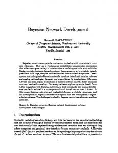
2.4 Difficulties in defining visual comfort entirely on the shipbuilder’s experience and prior work—or lack thereof. The Vasa swedish ship of the line was the most powerful ship of the world when launched from Stockholm on 10 August 1628—until it capsized and sank, less than 1000 m into her maiden voyage. Its complete design was in the head of the shipwright, based on shifting specifications given by the King. Now that shipbuilding has become a science, we know that if the ship’s center of gravity had been about 10 cm lower it would have remained afloat. Almost no discipline related to human welfare can today be called an exact science. Medical science is probably the most scientific-like of such disciplines, having also evolved from empirical roots, but remains even today a science that relies heavily on probabilities and statistics. Our eyes are not optimally adapted to life indoors, to its short distances, and in particular to its relatively low illuminances. The lighting in most of our modern workplaces, be they factories, hospitals, offices, shops or workshops, is unnatural and unsuitable for our natural condition. Understanding what makes an environment visually pleasant and healthy must therefore be regarded as a difficult, inexact discipline that has immensely benefited from science but that is still far from being completely consolidated. There is no formal, universally accepted way of quantifying visual comfort. If there was one, whose inputs were readily measurable quantities, a daylighting controller could be built provided one knew how to control those quantities. We will discuss the most popular proposals currently used in buildings codes in section 2.4.3 but first we will review early, more empirical work on this matter. Luckiesh and Moss (1937) is one of the earliest works on the topic of visual comfort still easily available. Their text summarizes research that was carried out during and after World War I, when it was important to maximize the industrial output from factory workers. The effect of lighting on productivity was one such parameter that was investigated during that time. The authors note that to establish a suitable visual environment one must ask oneself three questions: 1) What kind of light do we have? 2) How much of it do we have? and 3) What do we do with it? The first two questions deal with what kind of Light is available, while the third one deals with what Lighting we are to produce. Nowadays, the production of light of any quality and quantity is no longer an economic problem. Until 1880, mankind had to carry out most of its indoor activities with one-candela light sources, under conditions that would be considered intolerable today4 , whereas the cost of the lighting equipment in a modern building is a small fraction of the overall building’s cost. The challenges left to the designer of a lighting control system are therefore to provide a visual environment that makes human activities possible and comfortable with whatever lighting is available, while minimizing its energy consumption. In this work we will develop a controller for a pre-existing installation and there will be no guarantee that the office could not be lit in a better way, but the visual environment we provide will be the one that makes the optimal compromise between comfort and energy with the current lighting installation. A common metric used in lighting prescriptions is the illuminance of the surface where most of the work is being done. If this task illuminance is constant across the surface, it 4

But which unfortunately are still the norm in many countries. Luxtreks (http://www.luxtreks.com) is a not-for-profit organisation dedicated to donating solar-powered, battery-equipped lighting units to remote villages in places such as Bolivia, Peru or Tanzania. Their beneficiaries suffer often from lung damages caused by toxic fumes emitted from their crude ghee lamps (burning clarified butter) or kerosene lamps.

13

2 The need for integrated daylighting controllers in modern buildings must fall between two extremes: 1) an illuminance just sufficient for discerning the details of the work at hand, for the duration of the work; and 2) an illuminance that provides the easiest perception of the work surface. Any illuminance below this minimum will make the work impossible while any illuminance above this maximum is a waste of energy (and a risk of glare). We might be tempted to search for such an intermediate illuminance, balancing the energetic cost with the economic cost of having people not work in the easiest and most productive conditions, but this is impossible in practice. Instead, as we will see, our system will try to find a practical illuminance (retaining the terminology introduced by Luckiesh and Moss), that is, an illuminance that still permits productive and healthy work to be done while keeping energy expenditures low. It is, of course, slightly ironic to spend so much energy on achieving a given illuminance, which is something the eye is totally insensitive to. The brightness, or luminance of a surface, is what is directly perceived by the eye, and depends not only on the surface’s illuminance but also on its reflectance and specularity. For the relatively diffuse, homogenous surfaces usually encountered in the workspace we will assume that the luminance of a surface as seen by the observer is proportional to its illuminance. Luckiesh and Moss give one of the earliest tables of recommended illuminances for different tasks. They recommend 20–50 footcandles (fc), or 215–540 lx, for typical office work, i.e. “moderately critical and prolonged tasks, such as clerical work, ordinary reading [...]”. They also relate an experiment whereby 82 schoolteachers were asked to adjust the illuminance they deemed necessary for reading black print on white paper for extended periods of time. The results are shown in Figure 2.7. This experiment illustrates the extreme variations that can be found from individual to individual (a factor of 100 more illuminance in the extreme cases) and suggests that global illuminance prescriptions are not sufficient, but that illuminances should be adjusted for (or by) each individual. Luckiesh and Moss deal with adequate illuminances but provide little guidance on the avoidance of excessive lighting levels. At the time their book was written, daylight was not yet widely incorporated in building design, nor were electric lighting fixtures strong enough to cause serious glare problems. Weston (1935, 1945) has studied the relationship between task performance and task illuminance, especially above the visibility threshold. He has shown that in general, task performance increased first rapidly with task illuminance until a point is reached where large changes in task illuminance have only small effects. It is tempting to conclude that there is no reason to provide more task illuminance than that required for an efficient execution of the task—but a task illuminated just enough to carry it out cannot be sustained for prolonged periods of time. There is more to visual comfort than just the speedy execution of a short task. Etienne Grandjean has carried out important research in every aspect of comfort in the work environment, including visual comfort in the computerized environment. In Ergonomics in Computerized Offices (Grandjean, 1987) he defines glare as “a gross overloading of the adaptation processes of the eye, brought about by overexposure of the retina to light.” He further distinguishes between “relative glare”, caused by “excessive brightness contrasts between different parts of the visual field”; “absolute glare”, caused by sources so bright that the eye cannot physiologically adapt to them (e.g. the sun); and “adaptive glare”, a temporary effect experienced, for instance, when coming out of a dark room into bright daylight. He recommends that “All important surfaces withing the visual field should be of the same

14

2.4 Difficulties in defining visual comfort

25

Number of votes

20

15

10

5

0 100

200

500

1000

2000

5000

10000

Illuminance [lx]

Figure 2.7: Preferred illuminance among 82 schoolteachers, from Luckiesh and Moss (1937). The horizontal scale is logarithmic.

15

2 The need for integrated daylighting controllers in modern buildings order of brightness”, and that “The general level of illumination should not fluctuate rapidly because pupil reaction as well as retinal adaptation is a relatively slow process.” His work is one of the earliest works recommending spatial and temporal uniformity of luminances in the field of view, in addition to a suitable range of illuminance and avoidance of glare. He cites a study of 15 open-plan offices and 519 employees, where a workplane illuminance of 1000 lx or more resulted in a statistically significant increase in reported eye complaints. Employees preferred illuminance ranging between 400–850 lx. He points out that it is certainly not the workplane illuminance itself which was the source of glare. A brightly lit office room is rather more likely to have problems with reflections, deep shadows and relative glare. Experiments showing preferred illuminances between 1000–4000 lx should, according to Grandjean, be eyed with suspicion. Such findings could be artefacts that result from uncarefully designed brightly lit backgrounds. Grandjean recommends that office jobs without visual display terminals (VDT) should be illuminated by 500–700 lx, with brighter values for elder people. VDT tasks where most of the time is spent staring at the screen should be given 300 lx. These recommendations, however, were given at a time when computer screens were black with monochrome display and whose letters had luminances of 40–50 cd/m2 . It is not clear whether these prescriptions are still valid today. Refering to general lighting design and placement of luminaires, Grandjean gives the rules summarized in Table 2.4.1. Even today, reflections on computer screens are a major cause of discomfort. These should be avoided, and the single most effective measure one can take according to Grandjean is to adequately position the screen with respect to lights, windows and other bright surfaces. He concludes by recommending between 300–500 lx for conversational tasks, i.e. tasks during which one often glances at the screen, and 500–700 lx otherwise. Again, these values should probably be revised since the widespread introduction of high-luminance flat screens. Grandjean is also the author of Fitting the Task to the Man (Grandjean, 1988), whose chapters 17 (Vision) and 18 (Ergonomic principles of lighting) are of interest to us. These chapters pick up where his earlier book left off and complement it with more definitions and prescriptions. He defines “visual acuity” as the “ability to perceive two lines or points with minimal intervals as distinct”. Visual acuity is essentially what enables us to carry out our work efficiently and comfortably. It varies as follows: 1. It increases with the illuminance, plateauing at illuminances above 100 lx. 2. It increases with the contrast between the test symbols (letters on paper or on a screen) and their immediate background. 3. It is greater for dark symbols on a bright background than the reverse. 4. It decreases with age, down to about 50% at 80 years old. Since visual acuity does not greatly improve with higher illuminances, Grandjean cautions again against more than 1000 lx in office spaces and recommends task illuminances in the 500–700 lx range. Grandjean points out that the German (DIN) and American (IES, 5th ed, 1972) requirements for the same tasks are significantly different. The American values are systematically

16

High windows are more effective than broad ones, since the light penetrates further into the room. The lintel should not be deeper than 300 mm. Window sills should be at table height. If the window extends below the table-top it will be cold in winter and may cause glare. The distance from window to workplace should not be more than twice the height of the window. For workrooms the window area should be about one-fifth of the floor area. This is only a general rule which is very flexible according to circumstances. It is important that the glass should transmit plenty of light flux. Clear glass has a transparency of more than 90%, whereas frosted glass, glass bricks, or special heat-insulating glass may have transparencies from 70% down to only 30%. Effective protections against the glare of direct sunlight, and against radiant heat, are important in securing good visibility and comfort indoors. The most efficient method is an adjustable external sunshade, either venetian blinds or shutters. Venetian blinds inside the window, or between the panes of double-glazing, are a mistake, because they afford no protection against radiant heat. Each window should receive direct light from the sky vault, and it is desirable that a portion of sky should be visible from every workplace. The nearest building should be at least twice as far away as its own height. Pale colours should be used, both in the room itself, and in any courtyard outside, so as to reflect as much of the incident daylight as possible.

All large objects and major surfaces in the visual environment should, if possible, be equally bright.

The line from eye to light source must have an angle of more than 30° to the horizontal plane. If a smaller angle cannot be avoided, then the lamps must be shaded more effectively.

The working area should be brighter in the middle and darker in the surrounding field.

To avoid annoying reflections from the desk surface, the line from eye to desk should not coincide with the line of reflected light.

Surfaces in the middle of the visual fiels should not have a brightness contrast of more than 3:1.

Contrasts between the central and the marginal areas of the visual field should not exceed 10:1.

Light sources should not contrast with their background by more than 20:1.

The maximum brightness contrast within the entire room should not exceed 40:1.

No light source should appear within the visual field of an office employee during the working activities.

17

Table 2.1: Lighting design, luminaire placement, and daylighting design rules, from Grandjean (1987, 1988).

The use of reflecting colours and materials on table-tops or office machines should be avoided.

Excessive contrasts are more troublesome at the sides than at the top of the visual field.

It is better to use more lamps, each of lower power, than a few high-powered lamps.

Fluorescent tubes should be aligned at right angles to the line of sight.

All lights should be provided with shades or glare shields to prevent the luminance of the light source exceeding 200 cd/m2 .

Daylighting design

Lighting design and luminaire placement

2.4 Difficulties in defining visual comfort

2 The need for integrated daylighting controllers in modern buildings higher. The recommended illuminance for office work are a mere 500 lx in Germany but 1600 lx in the US. This should be taken as anecdotal evidence that official lighting recommendations do not depend only on genuine ergonomic principles, but also on political and economical ones, such as the price of energy. Fitting the Task to the Man concludes with design rules with respect to daylight, that we have also summarized in Table 2.4.1.

2.4.2 Preferred range of illuminance It should be kept in mind that lighting is not an exact science. It deals with people as well as things, and the lighting in a given interior is not good unless the occupants like it. An awareness of the fact that lighting is as much an art as a science is, indeed, central to a full appreciation of what is important in interior lighting. (CIE Guide on Interior Lighting, second edition)

In addition to the experiments described in the previous section, other researchers have conducted similar experiments where volunteers were asked to rate illuminances, in order to estimate what the optimal range of illuminance for typical office work should be. Fischer (1970) has pooled the results of such experiments conducted by Balder (1957), Muck and Bodmann (1961), S¨ ollner (1966), Riemenschneider (1967), Westhoff and Horeman (1963), Boyce (1968), and Bodmann et al. (1963). In each experiment the distribution of the reported preferred illuminances on a logarithmic scale have been fitted with a normal distribution. From these plots we have estimated the full width at half-maximum of each distribution and deduced the fitted standard deviation. The IESNA Lighting Handbook (Rea, 2000, page 3-39) gives some additional illuminance ranges from Bodmann (1962), Saunders (1969), Bean and Hopkins (1980) and Nemecek and Grandjean (1973), without specifying if these are confidence intervals, a fitted or sample standard deviation or the standard error on the mean estimate. For example, Nemecek and Grandjean report that: [...] the frequency of eye troubles in the three offices with more than 1000 lx was significantly higher than in the other ones (p < 0.001). Another analysis revealed that lighting intensities between 400–850 lx were judged to be the best. whereas Saunders report that: [...] at 400 lx, approximately 85% of the observers found the lighting conditions satisfactory or better, the figure increasing to 95% at 1000 lx. Figure 2.8 summarizes these findings, assuming the work quoted by the IESNA Lighting Handbook refers to the fitted standard deviation. The study due to Vine et al. (1998) was included in a similar fashion. Nabil and Mardaljevic (2005) have carried out one of the most recent reviews of the current understanding of preferred illuminances. They conclude that: ˆ Daylight illuminances lower than 100 lx are generally considered insufficient to be either the sole source of illumination or to contribute significantly to artificial lighting.

18

2.4 Difficulties in defining visual comfort

Study Balder Muck 1 Muck 2 Bodmann Westhoff Söllner Riemenshneider 1 Riemenshneider 2 Boyce Saunders Nemecek Bean Vine (morning) Vine (afternoon)

Year 1957 1961 1961 1962 1963 1966 1967 1967 1968 1969 1973 1980 1998 1998

Recommended value 100

200

500

1000

2000

5000

Workplane illuminance [lx]

Figure 2.8: Preferred illuminances in office rooms, pooled data. The width of each line is the fitted standard deviation, with some exceptions (see text). The size of each dot is inversely proportional to the fitted standard deviation. The vertical line is the recommended value of 500 lx one often finds in lighting design codes.

19

2 The need for integrated daylighting controllers in modern buildings ˆ Daylight illuminances in the range of 100–500 lx are considered effective either as the sole source of illumination or in conjunction with artificial lighting. ˆ Daylight illuminances in the range of 500–2000 lx are often perceived either as desirable or at least tolerable. ˆ Daylight illuminances higher than 2000 lx are likely to produce visual or thermal discomfort, or both.

From these observations they even propose a new measure of a building’s daylighting performance, christened “Useful Daylight Illuminance” (UDI), defined as the total time in the year the workplane’s illuminance is between 100–2000 lx. This range of illuminances was chosen precisely as a result of this literature review. They propose that this metric shall replace the Daylight Factor as an indicator of daylighting performance because: It is recognized that the daylight factor approach offers only a limited insight into true daylighting performance because it is founded on a measure of illumination under a single, idealized overcast sky. Figures 2.7 and 2.8 should make it clear that the range of preferred illuminances can vary greatly from individual to individual, a phenomenon recognized by Galasiu and Veitch (2006). Even within the restricted range of 100–2000 lx proposed by Nabil and Mardaljevic there is plenty of manoeuvering room for a lighting controller to achieve energy savings, instead of imposing a constant task illuminance on all occupants.

2.4.3 Objective quantification of visual discomfort and glare If there is a universal mind, must it be sane? (Charles Fort)

Throughout this work we will place much emphasis on the need to quantify objectively the visual discomfort. This notion might, at first, sound very odd. We are all very capable of determining by ourselves whether a visual environment is pleasant and productive or not, and nobody has ever walked around a building with an instrument measuring the visual discomfort (even though modern technology would in principle permit it). However, a rational assessment of visual discomfort is, in our opinion, important for three reasons. First, without such a tool, the building designers must rely on their expertise and rules of thumb to ensure that a planned building will satisfy the visual requirements of its future occupants. More often than not, these designers aim to satisfy national building construction codes that might fail to account for some peculiarity of the building, ruining in some cases the visual comfort. Second, daylight plays an important role in newly designed buildings because of the potential energy savings. But the use of daylight poses glare problems of its own that can be overlooked unless one quantifies objectively the visual discomfort. Third, the performance of most daylight-responsive control algorithms (including the present one) will benefit from a rational quantification of the visual discomfort. Coupled with an accurate daylighting model, the controller’s algorithm is free to explore its degrees of freedom and find the combination of blinds’ settings and electric lighting power that provides an optimal visual environment.

20

2.4 Difficulties in defining visual comfort In this section we will review the current understanding of this problem and the recommendations used by practitioners. Glare and insufficient illuminance are two main causes of visual discomfort in interior environments, but are usually treated separately in the literature and in building codes. Glare is, by far, the most difficult problem of the two. Early work by Guth and Hopkinson focused on finding a mathematical relationship between glare perception and the distribution, size and intensity of light sources. Field studies led to the determination of Guth’s Discomfort Glare Rating and to Hopkinsons’s Glare Index in the early sixties. The Commission Internationale de l’Eclairage (CIE) compiled these results in 1983 and published a report Discomfort Glare in the Interior Working Environment (CIE, 1983) on the state-of-the-art on discomfort glare5 in the interior working environment. In the same report, the CIE recommends the adoption of a formula proposed by Einhorn, considered as the best compromise between different national systems. This formula led to the CIE Glare Index (CGI), defined by: " # 1 + Ed /500 X L2s ωs CGI = 8 log10 2 · (2.1) Ed + Ei p2s s where Ed is the direct vertical illuminance [lx] at eye level from all sources, Ei is the eye-level indirect (excluding the glare source) illuminance [lx], Ls is the luminance [cd/m2 ] of the bright part of each source s in the direction of the eye, and ωs is the solid angle [sr] of the latter. ps is an index proposed by Guth that gives different weights to luminous sources according to their position in the visual field: sources close to the center of the field of view will carry more weight than sources in the field of view’s periphery. This index is defined by:  ps = exp (35.2 − 0.31889 · α − 1.22 · exp(−2α/9)) · 10−3 · β  + (21 + 0.26667 · α − 0.002963 · α2 ) · 10−5 · β 2 (2.2)

where α is the angle [rad] from vertical of the plane containing the source and the line of sight and β is the angle [rad] between the line of sight and the line from the observer to the source. This function is plotted in Figure 2.9. The CGI made it difficult, however, for luminaire manufacturers to provide design aids such as luminaire data sheets. This, and changes in the working environment, led in 1995 to the publication of another CIE report Discomfort Glare in Interior Lighting (CIE, 1995) in which the Unified Glare Rating (UGR) was introduced, defined by: " # 0.25 X L2s ωs UGR = 8 log10 (2.3) Lb s p2s

where Lb = Ei /π is the background luminance [cd/m2 ] seen by the eye of the observer. The UGR is thus a simplified version of the CGI in which no Ed appears, because “for the simplified glare calculation procedures [...] it has not been possible to find a way to include the direct illuminance.” 5

Discomfort glare is defined as glare that causes discomfort without necessarily impairing the vision of objects. It is distinct from disability glare, which is defined as glare that impairs the vision of objects without necessarily causing discomfort.

21

2 The need for integrated daylighting controllers in modern buildings

2 1.025

Y position [m]

1

1.020

1.015 0 1.010

−1

1.005

1.000 −2 −2

−1

0

1

2

X position [m]

Figure 2.9: Guth’s position index ps for a source on a plane 3 m away and perpendicular to the line of sight.

22

2.4 Difficulties in defining visual comfort VCP UGR

50% 24.0

60% 21.6

70% 19.0

80% 16.0

90% 11.6

Table 2.2: Correspondence between the UGR and VCP. The UGR takes on typically values between 10 and 30. One glare rating unit is the least detectable step, while three glare rating units are considered the finest granularity that makes sense for normative purposes. UGR = 14 and lower corresponds to the least perceptible glare effect. The standard recommends the UGR be rounded to a value belonging to 13–16–19– 22–25–28. The advantage of this new formula was its relative simplicity, which would help luminaire designers provide design aids and simplified glare calculation procedures. Today, however, both indices are readily available from computer simulations. The UGR is very popular among european lighting designers. American designers prefer the Visual Comfort Probability (VCP), whose expression is given in the IESNA Lighting Handbook (Rea, 2000) but is too involved to be reproduced here. The Handbook notes the correlation between this index and the UGR and recommends a table of correspondence between the two, given in Table 2.2. Neither the CGI nor the UGR has been validated against daylight glare or against large light sources. Glare from windows has been simulated in experiments at the Building Research Station in England and at the Cornell University in the USA, using fluorescent lamps behind diffusing screens. From these experiments, the “Cornell formula” (Chauvel et al., 1982) or Daylight Glare Index (DGI) has been derived, defined by: DGI = 10 log10 0.48

X s

Ls1.6 Ω0.8 s Lb + 0.07ωs0.5 Ls

(2.4)

where Ls is the source luminance [cd/m2 ], Lb is the background luminance [cd/m2 ], ωs is the solid angle of the source [sr], and Ωs is the solid angle [sr] of the source modified by its position in the field of view of the user. Even the DGI has been derived from electric lighting though, and Chauvel et al. (1982) found that a direct application of the DGI formula to a real daylit window overestimates the sensation of glare. For example, a daylit window that would in theory have a DGI rating of 16 is perceived to be about as glary as a luminaire whose DGI would be 10. Recent research by Tuaycharoen and Tregenza (2005) suggests that people are more tolerant towards visually stimulating sources of glare that carry some form of information, instead of plain white lights6 . The CIE, in its report Collection on Glare (CIE-2002), points out that the UGR yields glare estimates that are too severe for small (1.5 m2 ). For example, a straightforward application of the UGR for a 15 W incandescent lamp, 2 m above eye level, 4 m away, in 30 cd/m2 background luminance yields an UGR of 39, i.e. totally intolerable glare. According to this report, research has shown that for small sources in interior lighting it is the projected area of the source 7 , rather than its solid angle (which for small sources is the projected area divided by the distance), which should be used in the calculation of its 6

Which does not necessarily mean that the visual comfort is improved. The sensation of glare can be reduced without necessarily improving the visual comfort, in the traditional sense of “capacity to carry out some work efficiently”. 7 I.e., the area obtained by projecting the source on a plane whose normal is the line of sight.

23

2 The need for integrated daylighting controllers in modern buildings Illuminance [lx] UGR

300 13

600 16

1000 19

1600 22

Table 2.3: UGR for large glare sources. luminance. All small sources are therefore taken as being perceived as of size A = 0.005 m2 , or as discs 80 mm in diameter, no matter their distance to the observer. Therefore, their luminance L [cd/m2 ] shall be given as: L=

I = 200 · I A

(2.5)

where I is the intensity [cd] of the source. The summand in the UGR formula should therefore be replaced with: Is2 L2s ωs = 200 p2s rs2 p2s

(2.6)

where rs is the distance [m] to the source. This correction is valid for sources more than 5° off the line of sight at typical indoor lighting distances. For large glare sources, i.e. luminous ceilings, the standard does not recommend any glare formula at all but gives a table of illuminances the ceiling might provide together with their corresponding UGR rating. These values are given in Table 2.3. The report proposes a new glare index called the GGR, that redefines the UGR in order to make the transition between “normal” sources and large sources continuous:    Ed   2.55 1 + 220 0.18  8 log  GGR = UGR + 1.18 − (2.7) E d CC 1+ E i

where CC is the ceiling coverage, taking values between 0.15–1. The last glare index we will describe in this section is the Daylight Glare Probability index proposed by Wienold and Christoffersen (2005), defined as: ! X L2 ωs s −5 −2 + 0.16 (2.8) DGP = 5.87 × 10 Ev + 9.18 × 10 log10 1 + Ev1.87 p2s s

where Ev is the vertical eye illuminance [lx], Ls is the luminance of the source [cd/m2 ], ωs is the solid angle of the source [sr] and ps is Guth’s position index. They found this formula to correlate well with reported glare for DGP values between 0.2–0.8. The DGP estimates a glare probability as a function of the vertical eye-level illuminance8 and of the luminances of the most luminous sources in the field of view of the user, and has been derived from real, daylit windows. The inputs to this index are simple enough for this formula to be implemented in a commercial controller, provided outside solar conditions are known to the controller and some reasonable assumptions are made as to the layout of the 8

In Wienold and Christoffersen (2005), the authors measured this illuminance in a separate room adjacent to, and identical to, the one in which the subjects underwent productivity tests. The illuminance was measured close to the position where the subject’s eye would be.

24

2.5 Legislative efforts user’s environment (furniture, workplace disposition, etc), and as to the user’s location with respect to the windows. All these indices have been developed in an attempt to mathematically rate the glare sensation of an environment, but require a complete knowledge of luminance distributions in the field of view of the user. They are therefore difficult to use effectively in commercial controllers without at least installing a luminance mapper behind the user. Another limitation of these formulas is that they treat only visual discomfort caused by glare, and do not address visual discomfort caused by insufficient light. Used on their own, they are insufficient for the implementation of a lighting controller but have to be complemented by normative prescriptions with respect to illuminance distributions in the field of view of the user, such as the CIE recommendations (CIE, 1986). The formulas presented in this section attempt to quantify numerically the glare sensation or visual discomfort experienced by an average user as a function of lighting stimuli, leading to expressions that have grown increasingly complicated over the years. According to Kuhn (1996), a scientific theory that grows from an initial, simple formulation to layer upon layer of corrections and addendas is ripe for a paradigm shift, much as the geocentrism of antiquity whose simple initial expression failed to account for the observed planetary movements, and had to be completed with the unelegant theory of epicycles. More than once, a scientific theory has been adopted over competing theories because it was the simplest, and there is an unspoken feeling among some scientists that for a theory to be correct it must be elegant. Einstein would probably add that it should also be “as simple as possible, but not simpler”. Neither the UGR, GGR or any other glare formulas described in this section satisfy our definition of elegance or of simplicity, but more work in this field is certain to lead to a theory of visual comfort whose naturalness will be the best proof of its correctness. The theories we have today require too much knowledge of the user’s visual environment, and it is simply not practical to gather all this information. We do not have (yet) the necessary instruments that can evaluate the visual discomfort in realtime and feed that information to a daylighting controller. Besides, the current theories on visual comfort are statistical in nature and do not account for individual variations. The present work will, therefore, regress back to the way of empiricists and in chapter 5 we will develop a formalism for quantifying the visual discomfort by observing the behaviour of the user.

2.5 Legislative efforts Do you rulers ever give a just decision? (Psalm 58:1, Good News Translation)

In this section we will review the most important legislative documents relating to lighting comfort, control and energy management in buildings.

2.5.1 CIE Guide on Interior Lighting The Guide on Interior Lighting report from the CIE (CIE, 1986) refers to the study mentioned above by Fischer (1970) where people rated workplane illuminances. The horizontal illuminance was varied from 100 lx to about 20 000 lx. Three answers were possible: too dark, satisfactory or too bright.

25

2 The need for integrated daylighting controllers in modern buildings Illuminance range [lx] 200–300–500 300–500–750 500–750–1000

Type of task Tasks with simple visual requirements Tasks with medium visual requirements Tasks with demanding visual requirements

Table 2.4: Range of illuminance prescribed by CIE (1986) for different kinds of tasks. The middle value is the optimal illuminance. The standard concluded that: Practical experience has shown that an illuminance for general lighting of the order of 1000 lx is least likely to give rise to complaints, providing careful attention is paid to the avoidance of glare and to a proper balance of luminances of relevant surfaces in the room. The standard prescribes 20 lx as the minimum required for discerning features of the human face and is therefore considered as the absolute minimum for non-working interiors. Below 200 lx, most working interiors appear unacceptably dim. The standard ackowledges the logarithmic response of the human eye, and a 50% change in illuminance is considered the smallest increment in illuminance that results in a significant difference in subjective effect. This fact must be taken into account in tables of prescribed illuminances, as illuminance increments below this threshold are not perceptible. The standard gives a table with recommended illuminance ranges for different tasks, given in Table 2.4. The standard prescribes uniformity in task illuminance: the ratio of the minimum to the average illuminance of the workplane shall not be less than 0.8; the average interior illuminance shall not be less than 1/3 of the average workplane illuminance; and the average illuminance of adjacent interiors should not vary by more than a factor 5.

2.5.2 CIE Lighting of Indoor Work Places The Lighting of Indoor Work Places report from the CIE (CIE-2001) is a normative effort at standardizing lighting conditions in office rooms and other workspaces. It bases its recommendations on the UGR, and gives a table that prescribes a maximum UGR, a mean workplane illuminance, and a minimum colour rendering index for each kind of activity. For office rooms, CAD workstations and conference rooms the required mean illuminance is 500 lx, the maximum UGR is 19, and the minimum colour rendering index is 80. In circulation areas the required illuminance is 300 lx, the other requirements remaining unchanged. The daylight factor for interiors with side windows should not fall below 1% on the working plane 3 m from the window and 1 m from the walls. Supplementary lighting shall provide the required illuminance and balance the luminance distribution. This standard furthermore adds a clause limiting the luminance of overhead luminaires that might cause discomfort glare by reflections on VDTs. For class I and II screens (high quality screens, see ISO standard 9241-7), this maximum is 1000 cd/m2 . For class III screens, this maximum is 200 cd/m2 .

26

2.5 Legislative efforts The standard follows the one described in section 2.5.1 by prescribing task lighting uniformity, which shall not be less than 0.7, while the uniformity of the surroundings shall not be less than 0.5. The logarithmic sensitivity of the human eye to illuminances is reiterated in this standard, according to which, again, a factor of 50% is the smallest significant difference in subjective effect of illuminance. This was also mentioned as early as 1937 by Luckiesh and Moss, who pointed out that the human eye is sensible to relative differences of illuminances, not absolute ones, so that a change from 50 to 100 lx is perceived as equivalent to that from 500 to 1000 lx, provided the eye had had time to adapt before the increase. This norm has been adopted today as the european norm EN 12464-1:2002; the latter has been adopted as a swiss norm by the Schweizer Lichtgesellschaft.

2.5.3 European Parliament directive 2002/91/EC In December 2002 the European Parliament adopted directive 2002/91/EC (EC-2002), in recognition that: The residential and tertiary sector, the major part of which is buildings, accounts for more than 40% of final energy consumption in the Community and is expanding. The directive demands of Member States to establish national energy performance requirements for new and existing buildings, and to ensure that new buildings and buildings undergoing renovation are certified by independent energy experts. Boilers and air-conditioning systems must be regularly inspected. The directive does however not demand that control systems be taken into account.

2.5.4 Leadership in Energy and Environmental Design The Leadership in Energy and Environmental Design (LEED) Green Building Rating System is a US benchmark for “the design, construction, and operation of high performance green buildings”. It is a system of credits that assigns points to new or renovated buildings for meeting sustainable development goals. An intensive use of daylight and good views to the outside are part of LEED version 2.2 for new buildings. Credits 8.1 (Daylight 75% of Spaces, 1 point) is granted if: ˆ At least 75% of all occupied areas have at least 2% glazing factor9 , or ˆ Computer simulations demonstrate that at least 75% of all regularly occupied areas have 25 fc (about 250 lx) under clear sky conditions at noon on the equinox 30 in (about 75 cm) above the floor, or ˆ Measurements show that at least 75% of all regularly occupied areas have achieved at least 25 fc (250 lx). 9

Actual Tvis area The glazing factor is defined as Window ×Window geometry factor× Minimum ×Window height factor, Floor area Tvis but the free LEED rating system does not define these terms—we assume they are defined in the purchasable LEED reference guide.

27

2 The need for integrated daylighting controllers in modern buildings Credit 8.2 (Views for 90% of Spaces, 1 point) is granted if at least 90% of all regularly occupied areas have a direct line of sight to the outdoor environment via a glazing between 2’6” (76 cm) and 7’6” (229 cm) above floor finish. It is however unclear how venetian blinds whose slats are half-open should be accounted for.

2.5.5 ASHRAE 90.1-2004 ASHRAE publishes and maintains standard 90.1-2004, Energy Standard for Buildings Except Low-Rise Residential Buildings. The standard provides requirements for low-energy buildings and is intended to be adopted by local jurisdictions. It explicitly requires buildings of a certain size to be equipped with lighting control. Section 9.4.1.1 of the standard (Automatic Lighting Shutoff) states that: Interior lighting in buildings larger than 5000 ft2 (465 m2 ) shall be controlled with an automatic control device to shut off building lighting in all spaces. This automatic control device shall function on either: ˆ a scheduled basis using a time-of-day operated control device that turns lighting off at specific programmed times [...], or ˆ an occupant sensor that shall turn lighting off within 30 minutes of an occupant leaving a space, or ˆ a signal from another control or alarm system that indicates the area is unoccupied.

Section 9.4.1.2 (Space Control) states that: Each space enclosed by ceiling-height partitions shall have at least one control device to independently control the general lighting within the space. Each manual device shall be readily accessible and located so the occupants can see the controlled lighting. A control device shall be installed that automatically turns lighting off within 30 minutes of all occupants leaving a space [...] in classrooms [...], conference/meeting rooms, and employee lunch and break rooms. These spaces are not required to be connected to other automatic lighting shutoff controls. For all other spaces, each control device shall be activated either manually by an occupant or automatically by sensing an occupant. Each control device shall control a maximum of 2500 ft2 (232 m2 ) area for a space 10 000 ft2 (930 m2 ) or less and a maximum of 10 000 ft2 for a space greater than 10 000 ft2 and be capable of overriding any time-of-day scheduled shutoff control for no more than four hours. Provided these requirements are met the designer is relatively free to choose what system will schedule automatic lighting shutoff or decide that the space is no longer occupied.

28

2.5 Legislative efforts Very important Daylight integration and control Direct glare Luminances of room surfaces Reflected glare Important Color Appearance Flicker Light distribution on surfaces Light distribution on task plane (uniformity) Modeling of faces or objects Shadows Source/Task/Eye geometry Surface Characteristics Horizontal (500 lx) and vertical (50 lx) illuminances Table 2.5: Elements that contribute to visual comfort, according to the IESNA Lighting Handbook

2.5.6 IESNA Lighting Handbook The IESNA Lighting Handbook (Rea, 2000) is one of the most comprehensive handbooks available for the lighting designer. In its chapters on visual comfort, the Handbook uses the VCP as its visual comfort metric since it is this metric that is predominantly used in the US. Discomfort glare is deemed not to be a problem in a building if the VCP is 70% or more. Differences of 5 units or less are not considered signficant. In its appendices, the Handbook gives recommended illuminance ranges for a wide variety of activities. For “General offices, typing, computer rooms”, illuminances between 300–750 lx is recommended, 500 lx being optimal. In its section “Quality of the Visual Environment”, the Handbook lists the elements that contribute to visual comfort in a wide range of settings, and gives their relative qualitative importance. These elements are given in Table 2.5. Note in particular the very high importance granted to daylight integration and control for general offices, except for open-plan offices where this element is considered less important.

2.5.7 Swiss norms Swiss law requires not only that work spaces be sufficiently lit, it also requires that workers have an unobstructed view to the outside (OLT 3, art. 15, 24 and OLT 4, art. 17). Exceptions are allowed, but only if the work’s technical installations prevent the workers from having their view to the outside or for special cases, such as computer rooms or photo-processing laboratories. US-style cubicles are therefore illegal in Switzerland. Task illuminance, maximum UGR and color indices must follow the european norm EN 12464-1:2002 that we have previously discussed. The ratio between task luminance and immediate surrounding luminance must be kept lower than 3:1. The ratio between task luminance and general surrounding luminance must be kept lower than 5:1.

29

2 The need for integrated daylighting controllers in modern buildings

Zone Hours per year

Usage

Example

Office room 2750 h/year

300 lx, mostly daylight 500 lx, partly daylight 300 lx, no daylight

Private office room Bright office room Computer room

Consumption [MJ/m2 ·year] Maximum Target 35 12 70 40 90 60

Table 2.6: Maximum and target values for the electrical lighting energy consumption in offices according to SIA 380/4. Desired illuminance [lx] 50 100 200 300 400 500

Installed power [W/m2 ] Normal Strong 3.2 2.5 4.5 3.5 7.0 5.5 10.0 7.5 12.5 9.0 15.0 11.0

Table 2.7: Recommended installed power for electric lighting. Values are given for normal and strong energy performance requirements. The total glazed area of the building must, furthermore, be at least one eighth of the floor surface. At least half of that area must allow an outdoor view. Swiss norm SN 150911:1997 gives guidelines to building designers on how to integrate daylight in their designs. Illuminances and glare ratings are covered in Switzerland by the european norm EN 12464-1:2002, but the SIA (Soci´et´e Suisse des Ing´enieurs et Architectes) publishes recommendations for the HVAC and electric lighting energy consumptions. The 380/4 recommen´ ´ dation by the SIA L’Energie Electrique dans le Bˆ atiment gives maximum and target values for the electrical lighting energy consumption in different kinds of buildings. The values for office buildings are given in Table 2.6. This recommendation also provides limits on the installed electric lighting power. These limits are reproduced in Table 2.7. Typical values for expected yearly peak consumption hours are also given, and reproduced in Table 2.8. Zone Hours per year Office room 2750 h/year

Usage 300 lx, mostly daylight Partly daylight: 300 lx 500 lx No daylight

Peak consumption hours [hours/year] Normal Strong 1000 500 1200 1500 2750

900 1100 2400

Table 2.8: Typical consumption peak hours for electric lighting. Values are given for normal and strong energy performance requirements.

30

2.6 The need for an adaptive controller ´ The energy requirements for heating are covered in the SIA 380/1 recommendation L’Energie Thermique dans le Bˆ atiment. The limiting heating requirement for an administrative building are Qh = 75 + 90 × A/SRE [MJ/m2 ·year], where A [m2 ] is the ponderated sum of all surfaces of the building’s envelope (ground surfaces or surfaces adjacent to unheated zones being ponderated differently), and SRE [m2 ] is the energetic reference surface, the sum of all the building’s floor surfaces (with exceptions, given in the recommendation). For a typical administrative building, A/SRE = 0.8 and Qh = 147 MJ/m2 ·year.

2.6 The need for an adaptive controller Several normative documents acknowledge the difficulty of quantifying the visual discomfort for a large population. The IESNA Lighting Handbook (Rea, 2000), for instance, has studied the correlations between many of the glare indices described in section 2.4.3, and found that: All give reasonable predictions for the average discomfort of a group of people but give only poor predictions of an individual’s response. Similarly, the Guide on Interior Lighting report (CIE, 1986) states that: Because of this spread in glare sensation among people a quantity that is used to characterize the discomfort glare from a lighting installation is essentially a statistical quantity. It seems to this author indeed very odd that the equation defining the glare indices such as the UGR involve exclusively terms external to the observer; nowhere is there any dependency on variables inherent to the personal preferences or physiology of the latter. This author had recently to take out a new car insurance and was bombarded with highly personal questions designed to tailor a very specific insurance offer that would, presumably, minimize the risk to the insurer. It is mildly amusing to note how much effort is spent on getting to know the individual by insurance companies, while no such effort is apparent in the equations describing visual comfort nor, by extension, from building or lighting designers. The differences between individuals make it very difficult to frame a fixed set of rules that will fit all. As with thermal comfort, it is for all practical purposes impossible to satisfy everyone if the same control rules are uniformly applied. There is, however, a major difference between thermal and visual comfort. Fanger’s formalism for thermal comfort (now international standard ISO 7730) is widely held to satisfy 95% of users in the ideal case, and more typically 90%—leaving only 5–10% of users dissatisfied. But US standards, as we have seen, call for Visual Comfort Probabilities to be 70% or higher, implying that our current state-of-the-art in lighting design will typically leave 30% of users dissatisfied—or three to six times as many. Until we have a formalism for visual comfort whose satisfaction rate matches that of Fanger’s, we believe that any daylighting control system should apply different rules adapted to the preferences of individual users. We believe this is the only way that satisfaction rates higher than 90% can be achieved.

31

2 The need for integrated daylighting controllers in modern buildings

2.7 Difficulties in modeling daylighting with modern blinds A control algorithm that strives to maintain visual comfort while making an optimal use of shading devices (particularly if implemented on a low-powered, embedded controller) will work much better if it has an accurate, simple daylighting model of its lighting environment. The relative errors due to this model (i.e. the ratio between absolute error and real illuminance) must be smaller than illuminance differences the human eye can perceive. According to Luckiesh and Moss (1937), there is a geometric relationship between illuminance and perceived effect—doubling an illuminance from 100 to 200 lx is perceived approximatively as the same change from 1000 to 2000 lx. In addition, the illuminance “must be doubled to produce an obvious and significant improvement in seeing.”10 The IESNA Lighting Handbook (Rea, 2000) is more conservative and gives an illuminance change of 20% as the lowest detectable change. These elements suggest that in the absolutely worst case, a daylighting model for controllers cannot afford to be worse than 20% accurate, and 5–10% accuracy is a goal we should aim for. Few daylight modeling methods exist today that are both accurate and computationally cheap enough to be used on embedded hardware. A ray-tracing program such as Radiance (Larson and Shakespeare, 2003) is excluded because of its computational cost (especially when venetian blinds are involved), and a much simpler model is needed. The daylight factor (DF ) model assumes the indoor illuminance at a given point to be proportional to the outdoor, unobstructed, horizontal illuminance for a CIE Overcast Sky (CIE-1970)11 . This definition predicts accurate daylight illuminances only for CIE Overcast Skies. For such a sky, the indoor illuminance E is predicted by multiplying the daylight factor by the outdoor illuminance: E = DF × Eg hor (2.10) where Eg hor is the outdoor horizontal illuminance and DF is the daylight factor. The Daylight Factor method is one of two daylight illuminance calculation methods recommended by the IESNA Lighting Handbook (Rea, 2000). The Handbook recommends decomposing the DF into its sky component, its externally reflected component and its internally reflected component: DF = SC + ERC + IRC (2.11) The Handbook gives tables for hand-calculating these three components for a simple rectangular room under a CIE Overcast Sky, but warns that: The daylight factor is a low-precision procedure for determining the illuminance at any point in an interior space produced by a sky with a known luminance 10

This phenomenon should not come as a surprise to acousticians. The human ear is capable of operating across 12 orders of magnitude in acoustic energy. The human eye is likewise sensitive over 10 orders of magnitude. This extraordinary capacity is only possible with some kind of logarithmic response to the external stimuli—hence the geometric effect. 11 The CIE Overcast Sky—originally known as the Moon and Spencer (1942) sky—was adopted in 1955. It is a sky whose luminance Lθ [cd/m2 ] depends only on the height angle and whose zenith luminance LZ [cd/m2 ] is three times that at the horizon: Lθ = LZ

32

1 + 2 sin θ 3

(2.9)

2.7 Difficulties in modeling daylighting with modern blinds distribution. Direct sunlight is excluded. [...] It is used in northern Europe, where overcast skies predominate [...] The other method recommended by the Handbook is the so-called lumen method, which “assumes an empty rectangular room with simple fenestration and shading devices.” Furthermore: The procedure described here [...] does not provide for horizontal or vertical window blinds, nor for exterior elements such as sidewalks, streets, other buildings, and overhangs. In light of these limitations, we will not describe the lumen method here. As we will see in chapter 4, the DF model fails at predicting indoor illuminances for realistic sky conditions. Indeed, Robinson and Stone (2004) and many others argue that isotropic sky models (or models without azimuthal dependence, such as the CIE Overcast Sky) cannot accurately predict the vertical irradiance on a window. Such models do not take the sun’s position into account, and those errors will inevitably propagate on the calculation of the indoor illuminance. Guillemin (2003) has suggested that a better correlation than daylight factors might exist between indoor illuminances and vertical facade illuminance. He found experimentally that for the facades of our experimental building, the indoor illuminance could be modeled by E = a exp(b · α)Eg vert

(2.12)

where α (between 0 and 1) is the fraction of the window not covered by its textile blind, Eg vert is the facade’s vertical illuminance and a and b are model parameters to be fitted. For given blinds’ settings, the indoor illuminance is therefore assumed to be proportional to the outdoor vertical illuminance. Guillemin reports that the errors of this model have a standard deviation of 416 lx. We will also test this model in chapter 4 and see that it is insufficiently accurate for our needs. Moreover, this model was developed for textile blinds whereas our experiment will be carried out in offices equipped with one or two venetian blinds. Robinson and Stone (2006) have recently proposed a simplified indoor illuminance prediction algorithm that achieves very good accuracy, in particular in the presence of reflecting neighbouring buildings. However this model does not account for the particular reflecting characteristics of venetian blinds. Mahdavi (2001) is the only work we could find that describes a control system using a lighting simulation program, in this case, LUMINA. The paper describes a venetian blinds control system that tilts the blinds’ slats according to prescribed indoor lighting conditions and is very close to fulfilling our requirements. It is however not clear whether this control system is fast enough to run on a real controlled office. Spasojevi´c and Mahdavi (2005) report that an excellent indoor illuminance prediction can be achieved by segmenting the sky vault in 12 sectors and measuring the luminance of each sector. The luminance of each sector is then fed into the LUMINA lighting simulation program, instead of a complete sky luminance distribution function. For an office room with two unshaded south-east facing windows, the authors report a correlation between measured and simulated indoor illuminance of R2 = 0.89. But again, there does not appear to be any proof-of-concept implementation of this promising idea.

33

2 The need for integrated daylighting controllers in modern buildings Daylighting modeling methods based on so-called Daylight Coefficients (DC) have been shown to be accurate enough to compete with ray-tracing methods, and to be computationally light. Since they fulfill so many requirements for an embedded daylight controller we will defer their discussion to chapter 4, where our own daylighting model will be described. Were it not for one important shortcoming, DC methods would presumably have been adopted in this project. For the sake of completeness, Lehar and Glicksman (2007) have proposed an algorithm whose inputs are the geometry of the office and the distribution of reflectances in it. Each surface in the office is discretized into a mesh, and the brightness of each mesh element is given an initial brightness. The algorithm iteratively refines that guess until an equilibrium is reached and the brightness of each mesh element is a linear combination of the brightnesses of all other mesh elements. The authors found the algorithm’s computation time to be about 3–5 s (i.e. too slow for our application, where tens of modellings will be made at each time step) and that “roughly the same brightness levels are reported” between their model and a Radiance model. In light of this literature review it appears that no or few daylighting models exist that are fast enough to serve the needs of a real-time controller. As we will see in chapter 3, our controller will be tested against a real office room with two venetian blinds and against a virtual one with only one blind, so the daylighting model we need must be able to accomodate a variable number of venetian blinds. Such a model will be elaborated in chapter 4.

2.8 Recent control systems In this section we will review control algorithms that have recently been proposed in the academic literature, and that can therefore be taken as the state-of-the-art in daylighting control. Courret and Paule (1993) proposed a blinds control system that was to be fitted to the new Centre Suisse d’Electronique et de Microtechnique building in Neuchˆatel. The idea was to attach artificial retinas to each facade and to classify the sky condition as either overcast, intermediate or clear. A different control strategy is used for each sky condition. For overcast skies, the blinds are fully retracted. For intermediate skies, the blinds are completely lowered and their slats are opened. For clear skies, the blinds are lowered and the slat angle is chosen to optimize the protection against solar gains, the horizontal workplane illuminance, and visual comfort. The slat angle is calculated to always cut off direct sun, deemed to pose too large a risk of glare. Otherwise the slat angle is chosen to provide 300 lx throughout the room’s depth, and to keep the Visual Comfort Probability (c.f. section 2.4.3) above 70%. The authors use Radiance to calculate the illuminance and VCP profiles for different slat angles for different sun positions. The study concludes with the computation of a daily slat angle schedule for three typical days. The study is however completely theoretical in nature. The system has unfortunately never been implemented, nor its performance assessed. Lee et al. (1998) installed a dynamic venetian blind controller in an office room in Oakland (California), and monitored the energy consumption of that office compared to an identical one whose venetian blind was kept fixed (in the same position and slat angle) throughout the experiment, which lasted 14 months between 1996 and 1997. The daylighting controller adjusted the venetian blinds every 30 s to block direct sun and maintain the workplane illu-

34

2.8 Recent control systems minance at 540–700 lx. The system achieved lighting energy savings of 22–86% and cooling load reductions of about 28%. This study demonstrated the potential energy savings that can be achieved with a proper daylighting controller, even with one that “merely” keeps the workplane illuminance constant. Note in particular that the control algorithm makes no explicit attempt at minimizing solar gains during peak cooling periods; the cooling savings are achieved because peak cooling periods correspond usually to periods when the blinds need to be closed, resulting not only in a proper workplane illuminance but also in protection from solar gains. The same system was then assessed with 14 real occupants (Vine et al., 1998). Surveys found that 57% of respondents found the overall lighting to be comfortable, 29% found it uncomfortable, 71% of which because of insufficient daylight. We have alread mentioned in section 2.7 the daylight model used by Mahdavi (2001). In his paper, he also simulates the operation of a controller that uses this daylight model. His controller calculates at each timestep the value of a utility function for each combination of slat angle and electric lighting power, the optimal combination being then selected. This use of a utility (or cost) function is also the basis of the daylight controller we have developed in this work. It was also used by Ferguson (1990) in her thermal control algorithm. Guillemin (2003) has proposed a daylight control algorithm for office rooms equipped with two textile blinds based on a set of fuzzy rules. The variables that define the external environment (outdoor temperature, vertical facade illuminance, etc.) are discretized into categories and each possible combination is assigned an optimal blinds’ position. He found that 18 rules were necessary for a typical office room. The values of each rule are optimized daily so the controller can reproduce as closely as possible the blinds’ positions chosen by the users themselves. This algorithm is distinct from the previous ones in that it does not attempt to keep the controlled environment close to a design value, or the illuminances to prescribed values, or a glare index at a minimum. Instead, an expert judgment assigns initial values to each rule. If and when the user overrides the system, these rules are accordingly adjusted. This algorithm was shown to yield about 25% energy savings and to be accepted by 95% of the surveyed users (about 20 in all). The algorithm was implemented on the LESO experimental building (c.f. section 3.1), the same building on which the controller described in this work will be implemented. Variations on the theme of fuzzy logic control have been proposed by Lah et al. (2006) and Kolokotsa et al. (2006). In both cases, the control of a building is done through a set of fuzzy rules given initial values by a human expert. The work by Kolokotsa et al., in particular, is very close to the work described by Guillemin in that the fuzzy logic controller is implemented in Matlab and controls a building equipped with a commercial EIB system, which is exactly the conditions in which Guillemin worked. However, neither of these systems carries out any optimization of the rules nor takes into account user overrides. In spite of such promising results by machine-learning control algorithms, no commercial control system exists today that implements any of these ideas. Some innovative products are being rumoured, but even the daylight control system that will equip the New York Times Headquarters building, currently under constrution (Lee and Selkowitz, 2006), will limit itself to preventing direct sunlight and complement daylight with artificial lighting until a suitable workplane illuminance is reached (484–538 lx). The control algorithm described in this work is the first venetian blinds and electric lighting control algorithm proposed by our institute. Its underlying philosophy is different from that of

35

2 The need for integrated daylighting controllers in modern buildings the control algorithms described in this section, although it too attempts to minimize energy consumption while adapting itself to the user’s preferences.

2.9 Scope of this project This work was carried out as part of the Ecco-build project, whose goal was to develop and implement an adaptive control algorithm for venetian blinds and electric lighting, that minimizes the office room’s lighting and heating electrical consumption while maintaining the user visual comfort. We have implemented this algorithm on a pre-existing, real, occupied office while making sure it can also be run against a computer simulation of an office. The control algorithm will keep the office room’s energy consumption to a minimum, but learn from user overrides. No particular assumption has been made about the geographical location or orientation of the office, nor about its geometry or the distribution of its furniture. The location is an input to the algorithm but only for calculating the sun’s position. No parameterized model has been used in the visual discomfort estimation nor in the controller’s daylighting model, which is deduced from first principles. The controller has been implemented in a popular programming language used in embedded controllers. A limited number of mathematically complicated modules will use a compiled external mathematical library. Throughout this work we will not only discuss its theoretical principles but always keep an eye on a possible implementation on a commercial embedded controller.

36

3 Monitoring and simulation of controlled office rooms “What more do you want to know?” “The names of all the stars, and of all living things, and the whole history of Middle-Earth and Over-heaven and of the Sundering Seas,” laughed Pippin. “Of course! What else?” (J. R. R. Tolkien, The Two Towers)

In this chapter we will describe not only the office rooms on which our controller has been implemented, but also the computer model that helped develop and implement it, as well as assess its energy performance in different situations. Section 3.1 begins by describing the LESO solar experimental building, on which our controller’s implementation runs today. We will describe the two building office rooms that were fitted for that purpose and describe the hardware that has been installed. Section 3.2 then describes the computer model of a typical office room that was developed within this project, and that has been used for the development and assessment of the control algorithm and its implementation. As we will see, the computer program that implements the algorithm described in this work was designed to run indifferently against a real or a virtual office room. This is possible because that program is completely decoupled from the interface to the building automation system, which is replicated by the simulation program.

3.1 Office rooms description The LESO solar experimental building (Figure 3.1) is a middle-size (1000 m2 ) administrative building with 20 south-oriented office rooms of 15.7 m2 floor area each and height 2.8 m. Approximately half of them have a single user and the other half two. The south facade of the building was refurbished in 1999 with one that would satisfy sustainable development requirements, being made principally of wood and integrating advanced daylighting systems (so-called anidolic systems) that redistribute daylight in the offices (c.f. Figure 3.2). The LESO building is divided in nine thermically isolated units (three per floor). Most units have been partitioned in two office rooms. The conference room (LE 2 205) and the workshop (LE 0 05) are exceptions and occupy a complete unit each. The materials making up LESO’s construction elements are given in Table 3.1. The doors are 3.0 m2 in area and made of 2 cm thick wood. The lower windows are 2.1 m2 in area. The upper (anidolic) windows are inclined 45° and are 1.7 m2 in area. All windows (Silverstar N 13020 S glazing) are double glazed with IR coating, U-value 1.4 W/m2 ·K and gvalue 0.54. The windows’ frame is made of wood and its area is 0.9 m2 , its U-value 2 W/m2 ·K. The monitored total energy intensity of the building (including electric heating, lighting, computers and machines) is equal to 232 MJ/m2 ·year, of which 76 MJ/m2 ·year are needed for

37

3 Monitoring and simulation of controlled office rooms

Figure 3.1: The LESO solar experimental building in Lausanne, Switzerland.

Figure 3.2: The anidolic system of mirrors that redistribute daylight in LESO’s workshop.

38

3.1 Office rooms description

Element

Type

Area [m2 ] 5.4

South facade wall

Light wall

North wall (towards circulation area)

Heavy partition wall

7.0

Wall between units

Heavy partition wall

13.3

Wall within unit

Light partition wall

13.3

Floor

15.7

Ceiling (last floor)

15.7

Material Plaster panel Thermal insulation Wood Concrete bricks Thermal insulation Concrete bricks Concrete bricks Thermal insulation Concrete bricks Plaster panel Thermal insulation Plaster panel Rubber coating Screed Thermal insulation Concrete slab Concrete slab Thermal insulation Concrete and gravel

Thickness [cm] 1 12 1 12 8 12 12 8 12 1 4 1 1 6 6 25 25 16 10

Table 3.1: Materials and thicknesses of LESO construction elements. The external (west and east) walls have a 16 cm concrete bricks layer instead of 12 cm.

39

3 Monitoring and simulation of controlled office rooms heating space and 42 MJ/m2 ·year for lighting. The building is equipped with a grid-connected photovoltaic installation on its flat roof which provides 15.4 MJ/m2 ·year. Altherr and Gay (2002) have reported that the energy signature of the building when the outside temperature drops below 13°C (the so-called temperature of heating interlocking) is 0.72 W/m2 ·K. Above this temperature, the free (casual and solar) gains of the building are sufficient to heat it. The building has no active cooling or ventilation system except in one computer room. It is otherwise naturally ventilated by a stack effect. A detailed description of the building with its new southern facade, including an exhaustive analysis of the building’s energy flows, is given by Altherr and Gay (2002). The tasks carried out in these office rooms is evenly split between reading, writing, and work on the computer. The VDTs are mostly flat-screen monitors. The windows of all offices (except the ones used in this experiment) are protected by two external textile blinds. Floor drawings of the three building floors are shown in Figure 3.3. This building was used before its refurbishment for the experimentation of passive solar systems. Today it serves as test bench for advanced control algorithms for building services (heating, blinds and electric lighting). It is equipped with a commercial off-the-shelf European Installation Bus (EIB) building management system, with the following sensors and actuators: Outdoor sensors: outside air temperature, horizontal diffuse and global radiation, horizontal and south vertical illuminance, wind speed and direction. Indoor sensors (each office): air temperature, horizontal workplane illuminance, occupancy, and window opening. Indoor actuators (each office): blinds, electric lighting (continuous dimming), and electrical heating. User interface (each office): blinds, electric lighting, and indoor temperature setpoint. The electrical consumption of each room is also recorded. Each electrical meter has a rotating metallic disk on which a small (about 10°) sector is painted black. This disk is lit and rotates in front of a photodiode. When the black sector passes in front of the photodiode, a contact is broken, which is detected by a binary contact sensor connected to the EIB. The heating (“Force” meters) is recorded separately from the other appliances (“Lumi`ere” meters). Most Force meters are rated at 120 revolutions per kWh, and most Lumi`ere meters at 480 revolutions per kWh. No details are given on the meters about their precision, and we assume therefore conservatively an uncertainty of ±10 revolutions per kWh for both kinds of meters, i.e. a relative uncertainty on the energy consumption measurement of 8% for the Force meters and 2% on the Lumi`ere meters. The EIB building management system was installed in 1999. A PC is connected to that bus through a EIB-serial interface in order to run the control and monitoring program described in section 3.1.1. Since then, two research projects focused on control systems have been carried out using mesurements on the building, AdControl (Guillemin, 2003; Guillemin and Morel, 2003; Guillemin and Molteni, 2002) and Ecco-build. A data acquisition program has been running independently of any research project continuously since 2002 (except for upgrades). The data is stored in a MySQL database (MySQL Development Team, 2004, c.f. section 3.1.3), representing slightly more than five years of monitoring. For data related to user actions alone (change of occupancy, manual use of blinds or electric lighting controls, etc), we have accumulated at the time of writing about three million datapoints.

40

3.1 Office rooms description

Figure 3.3: Floor drawings of the LESO building. (0: basement; 1: first floor; 2: second floor.)

41

3 Monitoring and simulation of controlled office rooms

Figure 3.4: LESO office rooms equipped for this project. Office room 201 is to the left, office room 202 to the right. Two adjacent offices rooms (c.f. Figure 3.4) located on the second floor of the LESO building were equipped with venetian blinds in July 2004 and used in this study. The lower window was fitted with external blinds Baumann-H¨ uppe type “Noval 90”, bicolor slats RAL9016/RAL7035. The upper window was fitted with indoor1 blinds Baumann-H¨ uppe type “Genius 50” (c.f. Figure 3.5). Table 3.2 lists the devices installed in each of these two office rooms, as well as the equipment that monitors the outdoor environmental conditions. The horizontal workplane illuminance is measured with Siemens brightness sensors GE 252, which are actually ceiling-mounted luminance sensors shielded from the window’s luminance. The conversion from the workspace’s luminance to its illuminance is a programmable feature of the sensor, so that it can be calibrated to determine the illuminance, assuming a constant reflectance in its visual field. Each sensor has been calibrated with a reference sensor by Guillemin (2003). The sensors’ output is linear only up to about 500 lx, and has to be software-corrected in order to be accurate up to 3500 lx. Three additional illuminance sensors were installed in each office room used in this project, Wienold and Christoffersen (2006) having reported a good correlation between the glare sensation due to daylight and the eye-level vertical illuminance. Our control algorithm, described in chapter 5, is able to combine information from different sources and will adapt faster to the user’s preferences with three illuminance sensors instead of one. The first sensor was vertically installed at eye-level on the rear wall, slightly next to the user’s usual sitting place. The second one was placed on the opposite wall. The third sensor was placed horizontally about 15 cm above the user’s desks, giving an accurate reading of the workplane illuminance. The luxmeters provide an output current proportional to the intensity of the light flux impinging on them. A 100 Ω resistor was used to load them, allowing to read out a voltage (instead of a current). We calibrated them by placing their sensor under an adjustable light source, next to a reference illuminance sensor. The light source was gradually increased up to about 50 000 lx and the corresponding voltage was read out. The calibration curves are given in Figure 3.11. The sensors were then installed and connected to the GIRA Giersiepen analog sensor interface. One such sensor is shown in Figure 3.9. 1

The existing outdoor textile blinds, and the upper window’s slope, prevented us from fitting outdoor venetian blinds to the upper windows (which would have been a superior setup, from a thermal point of view).

42

3.1 Office rooms description

Figure 3.5: The blinds equipping office room 202. The upper indoor blinds are BaumannH¨ uppe type “Genius 50”, the lower outdoor blinds are Baumann-H¨ uppe type “Noval 90”.

Figure 3.6: Presence and ceiling-mounted luminance sensor.

43

44

AG ECO-IR 360AC-EIB UP 231/2 Delta profil GE 252 MX4 Analog-Sensorschnittstelle 4fach N 562 UP 220 JA/S4.230.1

BF3 Analog-Sensorschnittstelle 4fach MCR/PT100

In each office High Technology Systems Siemens Siemens BBC Goertz/Metrawatt GIRA Siemens Siemens ABB

Outdoor devices Delta-T GIRA Phoenix Contact

Sunshine sensor Analog/digital converter, 4 channels Temperature sensor

Presence sensor Push-button interface and temperature sensor (Il)luminance sensor Illuminance sensor Analog/digital converter, 4 channels Binary output (for heating control) Push button interface for blinds control Blinds actuator Force meter Lumi`ere meter

Type

12% ±0.5°C

°C

8% 2%

kWh kWh

W/m2

±0.5°C 15% 5%

Error

Boolean °C lx lx

Units

Table 3.2: Devices installed in office rooms 201 and 202 at LESO. Outdoor devices are also given.

Model

Manufacturer

3.10

3.7

3.6 3.8 3.6 3.9

Figure

3 Monitoring and simulation of controlled office rooms

3.1 Office rooms description

Figure 3.7: Venetian blinds manual controls.

Figure 3.8: Electric lighting and temperature setpoint control box. The user sets the electric lighting’s dimming levels with the two middle rockers. The leftmost rocker is used to select the temperature setpoint. The current temperature setpoint offset from 20° is indicated by the LED on the horizontal scale. The rightmost rocker is unused.

45

3 Monitoring and simulation of controlled office rooms

Figure 3.9: Wall-mounted illuminance sensor EB3 in office 202.

Figure 3.10: Delta-T BF3 sunshine sensor. A shading mask ensures that at least one of seven photosensitive diodes is always lit by direct sunlight, and at least one is shaded from it. The sensor can thus determine the diffuse and global components of daylight, and does not require any polar alignment (Delta-T Devices Ltd, 2006).

46

3.1 Office rooms description

0

EB4

50 100 150 200

EB5

EB6 60000

Illuminance [lx]

40000 20000 0

EB1

EB2

EB3

60000 40000 20000 0 0

50 100 150 200

0

50 100 150 200

U [mV]

Figure 3.11: Luxmeters calibration curves for the six luxmeters installed in office rooms 201 and 202. The luxmeters are labeled EB1, EB2 and so forth.

3.1.1 The Eibserver program The LESO building is equipped with a commercial building management system that can read out the status of the building’s sensors and actuators, and send commands to the latter. It was installed in 1999. As of August 2004, 240 sensors and actuators were on this system. Following the intial work of Ren´e Altherr, we have extended and currently maintain Eibserver, a Java program that allows a PC connected to the EIB system via its serial port to listen to, and send, EIB telegrams. It keeps in memory at all times the complete known state of the LESO building—when any variable is modified, that change is committed to memory and logged to disk (see section 3.1.2). Eibserver implements the Java Remote Method Invocation (RMI) mechanism to allow other processes, possibly running on remote machines, to subscribe for notification on specific events, to query the building’s status and to send control commands of their own. This can be done by any program implementing a Java virtual machine, including Matlab. But Matlab is unlikely to run on embedded devices in the foreseeable future (both for technical and economical reasons), whereas many Java virtual machines for embedded environments exist today2 . This is why we have tried to write as much of our controller in pure Java, as discussed in chapter 6. Below we give an example script written in Jython, an implementation of the Python programming language written in Java, with which we interactively query and send commands to the EIB system. Commands entered by the user are in bold: 2

E.g., http://www.skelmir.com/ or http://k-embedded-java.com/.

47

3 Monitoring and simulation of controlled office rooms

Figure 3.12: Interactive manipulation of textile blinds. The left photo is before sending the command, the right is after. The blind that moved is circled in red. 1 2 3 4 5 6 7 8 9 10 11

[lindelof@lesopriv3 ~]$ jython Jython 2.2a0 on java1.4.2_05 (JIT: null) Type "copyright", "credits" or "license" for more information. >>> from java.rmi import Naming >>> blind_201 = Naming.lookup("//lesopc7/bld-low_201") >>> blind_201.getPosition() 1.0 >>> blind_201.setPosition(0.2) >>> blind_201.getPosition() 0.2031 [lindelof@lesopriv3 ~]$ On line 5 we query the RMI server running on the same machine as Eibserver (i.e. lesopc7) for the remote object registered under the name bld-low_201, which is the lower textile blind in office 201. In the next lines the blinds’ position is queried, then set to 20% window’s fraction open, and queried again. The results, as seen by a webcam pointed at LESO’s south facade, are shown in Figure 3.12. As we will see, the remote interface exposed and implemented by Eibserver will also be implemented by the building simulation program described in section 3.2. Because this interface is common, it will be fully described in its own section 6.3.

3.1.2 Data logging The Eibserver program logs all bus events to disk. It first creates, if they do not exist already, subdirectories called lighting/, occupancy/, and so on in a results/ directory. In each of these directories, a new text file named DDMMYY.res (possibly appended with one or more tildes (~) if Eibserver had to restart that day) is created every night at midnight. The Eibserver program appends to these files the data as it comes in. The format of the data is, however, not quite consistent and has obviously evolved over time. Presently, according to comments left by the Eibserver program’s original author, that format is DDMMYY:HH:MM:SS;device_room;value where device is the name of the devices,

48

3.1 Office rooms description Table name luminosity skyluminosity consumption occupancy temperature blind heating lighting window setpoint

Description Indoor illuminance [lx] Outdoor illuminance [lx] / irradiance [W/m2 ] Electrical meters [kWh] User presence [boolean] Indoor and outdoor temperature [°C] Textile and venetian blinds’ positions and slat angles [0–1] Electrical heating power [%] Artificial lighting power [%] Windows open/closed status [boolean] User-chosen temperature setpoint [°C]

Records 26 946 119 20 994 794 5 238 006 2 986 328 2 722 403 976 656 803 075 379 339 64 104 5 508

Table 3.3: The tables in the ‘leso_eib’ database. The rows are sorted by decreasing number of records. The table names are identical to the names of the data directories created by Eibserver. The number of records are as of April 2007. possibly prefixed with usr: or set:, and possibly suffixed with _stat, _pos or some other descriptive string. room is the room number (3 digits), and value is the numeric data. Note in particular that according to the prefix of the device’s name one knows whether it was a user action or a command sent through Eibserver. It is thus possible to distinguish controller commands from user commands. Early data, however, presents difficulties. In rare cases the line is unrecoverable gibberish. Occasionally, race conditions allowed a thread to write out its data while another one was looking up the operating system’s definition of a newline, yielding two data entries on the same line followed by two newlines. These problems were rare and have not occured anymore.

3.1.3 The ‘leso_eib’ database We have written a Perl script (see Appendix C.1 for the source code) that starts every night at 5 a.m.3 , reads in the logfiles that have been written that day since midnight (one per subdirectory), parses each line, and inserts the corresponding values in a MySQL database. After reaching the end of each file the program checks every minute whether new data is available in that file, and updates the database accordingly. It stops at midnight. The MySQL database includes also all the data recorded by Eibserver since it began recording data in 2002. The database is made up of ten tables (sharing an identical structure), corresponding to the ten categories of data that Eibserver records. These tables and their schema are given in Tables 3.3 and 3.4. The database is accessible from a web interface, available on the EPFL intranet from http://lesopc28.epfl.ch/~lindelof/phpMyAdmin/index.php. From this interface users have read-only access to the entire database, and can dump portions of the data as text files. The main interface is shown in Figures 3.13 and 3.14. The database can, of course, also be programatically accessed. 3

All textile blinds are fully retracted by Eibserver at 2 a.m. and lowered again to their previous position. This ensures that any drift in the measurement of the blinds’ position is kept to a minimum. The Perl script starts at 5 a.m. to be sure that no other “administrative” process runs on the LESO building.

49

3 Monitoring and simulation of controlled office rooms

Field index date time room type device action data

MySQL Type int(11) date time char(3) varchar(5) varchar(20) varchar(5) double

Description Record index Date of the record (YYYY-MM-DD) Time of the record (HH:MM:SS) Office number (3-digit number, 300 for outdoor events) Source of the event (user, controller, sensor) Device name Kind of event (sensor, actuator command, etc.) Numeric data

Table 3.4: Schema of the ‘leso_eib’ database’s tables.

Figure 3.13: The main interface to the ‘leso_eib’ database.

50

3.2 Simbad model

Figure 3.14: Browsing a table of the ‘leso_eib’ database.

3.2 Simbad model One of the goals of this project is to demonstrate through computer simulations the potential energy savings with a blinds and electric lighting controller. To that end it was important to choose and, if need be, extend a building simulation package. Many software packages exist that model and simulate the thermal behaviour of building elements. The U.S. Department of Energy’s website4 lists at the time of writing 344 of them. ESP-r5 and EnergyPlus6 are the most popular packages in Europe and USA respectively. In this project we needed a software package that would model the thermal and visual aspects of an office room whose electric lighting and blinds are computer-controlled. We also required that the existing controller implementation could be easily coupled to this simulator. Simbad (SIMBAD-2006) is a Matlab toolbox for building simulation developed by the french Centre Scientifique et Technique du Bˆatiment (CSTB). It models most HVAC systems within a building but comes with no accurate daylighting model for a complex system such as venetian blinds. Simbad had, however, two very desirable features. First, as a Matlab toolbox, it is a library of simulation blocks for Simulink, the graphical tool for modeling and simulating dynamic systems under Matlab. Assembling a building model is very easy in this environment. Simbad provides out-of-the-box blocks for many building appliances such as heating elements or ventilation systems. Second, Simulink runs under Matlab, which has its own Java virtual machine. Java classes can therefore be loaded in Matlab and interact with the Matlab environment. Since 4

http://www.eere.energy.gov/buildings/tools_directory/ http://www.esru.strath.ac.uk/Programs/ESP-r.htm 6 http://www.energyplus.gov/ 5

51

3 Monitoring and simulation of controlled office rooms

Figure 3.15: Radiance model of the virtual office room. our controller’s implementation is completely decoupled from the interface to the building management system, we can write an interface in Java to our Simbad model that masquerades as the real building, and our controller will not see any difference. The benefits of this approach cannot be understated. Again: as long as we have a welldefined interface to the controlled systems, we are free to implement any control algorithm in any dialect of Java. In particular, we can write prototypes in Python using Jython7 (a Python implementation written in Java), or Groovy8 (a scripting platform for the Java language). This implementation can then run against Eibserver or against Simbad, since they both present this well-defined interface. As we will see, this led to dramatically short development cycles where programming defects were quickly discovered with the simulator and fixed before the real office room’s controller software was updated. The interface used in this project is described in section 6.3, but this idea of a common controller interface for any building management system will be elaborated further in Appendix A. The full details of our office room model are given by Marty and Fontoynont (2006). In the following we will discuss the elements of this model most important to us: the daylighting model, the user behaviour model and the heating/cooling model. The interface to the controller will be described in section 6.3.

3.2.1 Daylighting and electric lighting model The virtual office room is a cuboid 4.61 × 3.62 × 2.85 m3 in volume, with one side almost fully glazed and protected with venetian blinds. Figure 3.15 shows the Radiance model of this office room. 7 8

http://www.jython.org/Project/index.html http://groovy.codehaus.org/

52

3.2 Simbad model

800

100

Horizontal workplane illuminance [lx]

90 80

600

70 60 400

50 40 30

200

20 10 0

0 0

50

100

150

200

250

Electric power [W]

Figure 3.16: Simbad electric lighting calibration. The numbers represent the lighting command in % sent to the Simbad block. The electric lighting model consists of six 36 W fluorescent tubes (or 12.94 W/m2 installed power density) with a 95 lm/W efficiency and a 20% time depreciation factor. The ballasts in this model are assumed to be responsible for a 15% overconsumption (about 30 W). The office room is 16.7 m2 in area and has an 80% utilance factor, so the electric lighting can provide an illuminance anywhere between 0–780 lx9 . This high upper limit was deliberately chosen to see whether the controller would correctly limit the illuminance to more reasonable levels. We have used a Python script to increase the lighting command in steps of 10%, and read out the electric power consumption and resulting illuminance. The result is shown in Figure 3.16. For the daylighting model, we briefly considered a daylight coefficients approach10 , whereby we would compute the coefficients for every blinds’ position, slat angle and illuminance sensor position combination. We would then also have had to implement a sky model in Simbad, but because of time pressures we decided instead to precalculate every possible illuminance 9 10

6 × 36 × (1 − 0.2)/16.7 × 80% = 786 lx. Daylight coefficients will be discussed again together with the controller’s daylight model, and defined in chapter 4.

53

3 Monitoring and simulation of controlled office rooms Column 1 2 3 4 5 6 7 8

Units NA NA NA lx lx lx lx lx

Description Month (January=1) Day of the month Hour of the day (with fractions) East wall illuminance West wall illuminance East eye-level illuminance West eye-level illuminance Workplace illuminance

Example 6 4 9.292 (09:17:30) 255 714 2584 3064 1373

Table 3.5: Precalculated illuminance file format. The examples come from file illum_v001_0_0_N.ill. The wall illuminances are calculated 2.1 m away from the facade, at a height of 2.15 m. The eye-level illuminances are calculated 2.1 m away from the facade, at a height of 1.2 m. The workplane illuminance is calculated 2.1 m away from the facade at a height of 0.8 m. for each timestep, office room location, office room orientation and blinds’ settings. This Radiance-based daylighting model consists of precalculated illuminances at five different positions in the virtual office room, for each minute of a year, with weather data files for Brussels (Belgium, 50°52’ N 4°22’ E) and for Rome (Italy, 41°54’ N 12°27’ E). These annual simulations were carried out for three different office orientations (south, west, and north). A roller blind or a venetian blind was added to the simulated model, and different simulations were made for different discrete blinds’ settings. 785 annual simulations were carried out, each yielding the five illuminances for every minute for the 525 600 minutes in a year. Each file is 32 megabyte large, and the whole data set represents 24 gigabytes. Jan Wienold of Fraunhofer-ISE carried out the simulations with the Radiance-based Daysim (Reinhart, 2006) program on a cluster of more than 50 nodes. The weather data was provided by Fraunhofer-ISE, who produced it with the Metenorm (METEONORM-2006) program. Daysim models the sky luminance distribution from global and direct outdoor horizontal illuminances with Perez’s all-weather sky model (Perez et al., 1993). Table 3.5 gives the structure of these precalculated illuminance files. A full illuminance simulation with meteorological data thus yields a table with 535 600 rows, whose structure is given in Table 3.6. The naming scheme for these files in given in Appendix C.2.

3.2.2 User behaviour model The virtual user is present in the office from 8 a.m. to noon, and from 2 p.m. to 6 p.m. during weekdays, and absent on weekends. No other holidays are modeled. The Simbad model runs with either the simulated user controlling the blinds and the artificial lighting, or the external controller, but not both. The user does not act on the office room controls at all while the automatic controller runs, but follows the same occupancy schedule. When the user controls the blinds, an algorithm, that follows a recent state-of-the-art review of users’ manual blinds control (Marty et al., 2003; Reinhart and Voss, 2003), determines the blinds’ position and slat angle:

54

3.2 Simbad model Field index time Eeg Eed Eev Ees temperature rightWall leftWall rightEye leftEye horiz elevation azimuth clearness clearness.cat

Units N/A POSIX time W/m2 W/m2 W/m2 W/m2 °C lx lx lx lx lx ° ° N/A N/A

Description Datapoint index Timestep Horizontal global irradiance Horizontal diffuse irradiance Vertical global irradiance Direct normal irradiance Outside temperature Right wall illuminance Left wall illuminance Right user position eye-level illuminance Left user position eye-level illuminance Horizontal workplane illuminance Solar elevation Solar azimuth (0° is north, 90° is east) Perez clearness ǫ Perez clearness category ǫ˜

Example 300000 2006-07-28 08:59:30 341 118 67.6 515 16.0 249 629 2542 3007 1398 25.7 91 2.76 5

Table 3.6: Structure of the simulated data. The Perez clearness ǫ and clearness category ǫ˜ will be defined in chapter 4. The names of the fields are the same as the ones used in the analysis code (Appendix C.1). ˆ At dawn and sunset, the blinds are completely up. ˆ If direct sun is present, the slat angle is adjusted to the cut-off angle (adding 5° if the slat angle was less than the cut-off angle). The height is adjusted so the sun patch is at least 50 cm away from the user. ˆ If the vertical illuminance on the facade is larger than 49 klx, the blinds are pulled completely down and the slat angle is adjusted to the cut-off angle (adding 5° if the slat angle was less than the cut-off angle).

When the user does any of these, no more actions can occur for 15 min. For these purposes, direct sun is considered present if the ratio global/diffuse irradiance is larger than 1.25 and the horizontal global irradiance is larger than 24 W/m2 . This definition is used internally by our BF3 sunshine sensor, and is known (Delta-T Devices Ltd, 2006) to correlate well with the World Meteorological Organisation’s definition (beam irradiance > 120 W/m2 ). The electric lighting is switched on by the user to maintain a desktop illuminance of at least 500 lx. The user can adjust the electric lighting power in steps of 33%. The user never decreases the electric lighting power before leaving the office (at noon or in the evening), when the lighting is switched off. This might sound harsh, but we have recently studied the so-called intermediate light switching probability by the LESO users, i.e. the probability as a function of indoor illuminance that the users switch their lights off without leaving the office. That study (Lindel¨of and Morel, 2006) found that whereas the intermediate switch-on probability for a 15-min timestep can be between 1% and 3% for workplane illuminances lower than 200 lx, the switch-off probability

55

3 Monitoring and simulation of controlled office rooms Name Inputs T°ext CMV flow H/C flux Int gains Solar flux Outputs Air T° w

Description

Units

Outdoor temperature A vector representing controlled mechanical ventilation and infiltrations Heating/cooling loads Internal heat gains Solar heat gains

A vector containing the characteristics of the room’s air, including its temperature Wall temperature

°C

W W W

°C

Table 3.7: Inputs and outputs to Simbad’s thermal model. does not depend on the illuminance and is lower than 0.2%. That study found also that most LESO users did not bother dimming their lights but turned them either fully on of fully off. A modeled user that never switches the lights off before leaving the office is, therefore, not worse than the average LESO user11 . Allowing the modeled user to dim the lights is, energetically speaking, an improvement. We therefore believe that our user model is fair, or even optimistic, and that our controller will be compared with an energy-conscious manual behaviour, not with a hopelessly irrational and wasteful one.

3.2.3 Heating and cooling model An 1000 W electric heater was added to the office model with a simple, independent controller that turns it on if the temperature decreases below 21° and turns it off when the temperature increases above 23°12 . The heater’s electric consumption is separetely recorded. A fancoil with water alimentation was also added to the model for cooling. It switches on if the temperature goes above 26°, and increases in power according to the current temperature. Its power consumption is also recorded.

3.2.4 Thermal model The office room’s thermal behaviour is modeled with a Simbad two-node thermal ‘Office room, medium inertia and high insulation’ block. One node is the indoor air temperature, the other is the wall temperature. The inputs and outputs of this model are given in Table 3.7. For each node, Simbad solves at each timestep the following equation: Ci

dTi (t) = −Gi ∆T (t) + qi (t) dt

(3.1)

where Ti (t) [K] is the temperature of node i, Ci [J/K] is the heat capacity of node i, Gi [W/K] is the heat flow conductance between the two nodes, and ∆T [K] is the temperature difference 11

The average LESO user will, however, leave the office room more often than only twice a day, increasing the probability of switching the lights off when they are not needed. 12 Note that more energy-conscious values would be 19° and 21° respectively.

56

3.3 Chapter summary between the nodes. q(t) [W] is the sum of the solar or casual gains, and of the heat losses, at node i, including any heat exchange with outdoors. In modern building simulation software, this equation is solved for a much higher number of thermal nodes—a common practice is to have at least three nodes per wall, one for each surface and one in the middle. For multi-layered construction elements, the number of nodes is even higher. The computation time being polynomial in the number of nodes, a reasonable balance between accuracy and speed must be struck. Our goal here is not to model the energy performance of a real office room, but rather to compare the energy performance of a simplified room under two different control strategies. As such, absolute accuracy is not required as much as relative accuracy. Adding more nodes to the model would increase its absolute accuracy but is unlikely to shed more light on the relative performance of one control strategy over another. A two-node model is, therefore, satisfactory for our needs. For a thorough discussion of building simulation, we recommend Clarke (2001). Ferguson (1990) discusses also, in her thesis, the pros and cons of different thermal node placement strategies.

3.2.5 Solar gains model The Fraunhofer Institute for Solar Energy (ISE) has carried out calculations (Kuhn, 2006a,b) of the total solar energy transmittance, or g-value, for different blinds used in this project. The calculations yield the g-values as a function of the source’s azimuth and elevation (which can be negative for ground reflections) and of the slat angle. This data was used in the simulation to calculate the free gains due to solar gains. The source’s azimuth was discretized between −80° and +80° in steps of 20°. Its elevation was discretized between −85° and +85° in steps of 5°. The slat angle was discretized between 0° (horizontal slats) and 75° (closed slats) in steps of 15°. The ISE produced one file per slat angle for each blinds. This data includes the glazing’s g-value (75% for the simulated office room, 63% for the LESO glazings). File epfl_genius_noval_ext_30.dat, for example, contains a 35 × 9 matrix with the g-values for the Noval blinds (c.f. Figure 3.5) tilted at 30° in front of LESO’s glazing. The data in this file is shown in Figure 3.17. The Simbad model assumes the office room’s windows to be Pilkington insulight 4/12/4 glazings (g-value 0.75). The model includes outdoor blinds, taken to be of the same model (and g-value) as the indoor Genius blinds fitted in LESO’s office rooms.

3.3 Chapter summary In this chapter we have seen in what office rooms and on what hardware the control algorithm will run. Two office rooms of the LESO building have been fitted with venetian blinds, whose sensors and actuators have been included in the existing EIB building management system. Each office room is fitted with three additional illuminance sensors. The program that interfaces between the control program and the building management system runs on its own dedicated machine, independently of the control program. Its public interface can be implemented by a computer program simulating the dynamic behaviour of an office room. We have built such a computer model with Simbad and given all of its characteristics.

57

3 Monitoring and simulation of controlled office rooms

80 0.6

70 60 50

0.5

40 30 0.4

Elevation

20 10 0

0.3

−10 −20 0.2

−30 −40 −50

0.1

−60 −70 0.0

−80 −80

−60

−40

−20

0

20

40

60

80

Azimuth

Figure 3.17: g-values for outdoor Noval venetian blinds with slats tilted 30°.

58

3.3 Chapter summary Our control program was written in Java and compiled against Eibserver’s public interface given in section 6.3—not one line of Eibserver’s code, or of any other building management system, or of Simbad is present in our controller’s code. The ability to run our controller indifferently against a real building or a virtual one was not planned for at the beginning of the project—it arose spontaneously once it was realized that Eibserver’s public interface could be separated from its implementation. We find ourselves today in favourable conditions for the development of further control algorithms. A careful algorithm developer will first implement it in a prototyping language and run it against the computer simulation. After it has been shown that the implementation is correct and produces the expected results, the algorithm can be implemented in Java, assessed again against the simulation, and finally run against a real office room. This setup should dramatically shorten the development time for future control algorithms on the LESO building.

59

3 Monitoring and simulation of controlled office rooms

60

4 Daylighting model In this chapter we will discuss the development of a simplified daylighting model suitable for embedded controllers. The main purpose of this model is to provide a daylighting illuminance prediction method for the controller described in chapter 6. As we will see, our control algorithm evaluates the visual discomfort as a function of the illuminance observed at different points in the office room. A daylighting model is therefore needed if we are to find blinds’ and electric lighting settings that minimize this visual discomfort. A model that predicts daylighting illuminances for arbitrary zones and arbitrary shading devices is, however, also a valuable tool for many proposed control algorithms. For this reason, we document this model independently of the visual discomfort model described in the next chapter. The model described in this chapter could (and should) be easily implemented as an independent software module, capable of providing a daylighting model as a service to other software modules running on the same platform. For these reasons, this chapter is mostly self-contained and can be read in isolation. Section 4.1 begins with some introductory remarks. In section 4.2 we discuss the Daylight Coefficients model, a model that would have been adopted for this project were it not for some critical shortcomings. In 4.3 we will first verify whether commonly used daylighting illuminance prediction methods are accurate enough for a daylighting controller. We will see that daylit scenes where direct sun is present cannot be accurately modeled with such models. In section 4.4 we will develop a linear daylighting model, valid for a given sun position. From this model we will deduce a more general one, which uses the history of past illuminances to assess the present illuminance. This model will be trained with a subset of simulated daylighting data, and validated on the remaining subset, in section 4.5. Finally, in section 4.6, we will build a working prototype controller set to maintain the horizontal workplane illuminance close to 500 lx and assess by simulation its performance over one year. Glossary Ein hor Eg hor Eg vert Ig hor Idiff hor Ibeam Idir hor DF ǫ ǫ˜ θ φ φf

Indoor horizontal illuminance [lx] Outdoor global horizontal illuminance [lx] Outdoor vertical facade illuminance [lx] Outdoor global horizontal irradiance [W/m2 ] Outdoor diffuse horizontal irradiance [W/m2 ] Direct beam irradiance [W/m2 ] Direct horizontal irradiance [W/m2 ] Daylight factor Perez sky clearness Perez sky clearness category Sun elevation [°] Sun azimuth (0° is north, 90° is east) [°] Facade normal azimuth [°]

61

4 Daylighting model

4.1 Model requirements Many control algorithms that strive to maintain visual comfort while making an optimal use of shading devices (particularly if implemented on a low-powered, embedded controller) need a simple and reliable daylighting model of the space being controlled. How accurate does this daylighting model need to be? Keep in mind its purpose: to help our controller predict illuminances on selected room surfaces, and to help it achieve appropriate illuminances. The human eye will therefore be the yardstick which will define how precise we need to be. The relative errors due to this model (i.e. the ratio between error and real illuminance) must be smaller than illuminance differences the human eye can perceive. We have seen in section 2.7 that this ratio lies between 20–50%, but our target precision should be closer to 5–10%. But we have also seen that few daylighting modeling methods exist today that are both accurate and computationally cheap enough to be used on embedded hardware. This chapter describes such a simple daylighting model intended for embedded daylight controllers. It provides a reasonably accurate prediction for daylighting illuminances for a controller that monitors the indoor illuminance on one hand, and the outdoor horizontal global and diffuse irradiance on the other hand. When asked to predict what illuminance would result from a given blinds’ settings, the algorithm looks back in time and retrieves illuminance measurements that have been taken when the blinds were in a similar setting and the sun was close to its current position. This indoor illuminance is then modeled as a linear combination of the outdoor horizontal global and diffuse irradiances, and the current illuminance is predicted from this linear fit. It is difficult, if not impossible, to develop, train and validate a daylighting model with real data. Experiments involving daylight are by nature impossible to repeat, and acquiring enough data takes far too long. We have therefore used Radiance-generated illuminances for different locations in a virtual office for each discretized venetian blinds’ position and slat angle and for each minute of a year. This data was described in section 3.2.1, and the daylighting models evaluated in this chapter have, as far as possible, been validated against this data set.

4.2 Daylight coefficients The Daylight Coefficients (DC) method, originally introduced by Tregenza and Waters (1983), is a method to completely characterize the illuminance response of an indoor point for an arbitrary sky luminance distribution. The idea is to divide the sky vault in discrete, non-overlapping sectors small enough for the sky luminance to be considered constant across that sector. One usually follows Tregenza’s division (Tregenza, 1987) into 145 non-overlapping circular zones between 11–12° in diameter. The dimensionless daylight coefficient Di for sky patch i is then defined for an indoor point by: ∆Ei Di = (4.1) ∆Ωi Li where ∆Ei [lx] is the total (direct and reflected) illuminance at the point from sky patch i, Li [cd/m2 ] is the luminance of the patch, and ∆Ωi [sr] is its solid angle. The product Di ∆Ωi is thus the proportionality coefficient between the illuminance at the point and the luminance of the patch (c.f. Figure 4.1). It measures directly how much the luminance of that sky patch

62

4.2 Daylight coefficients

Li

∆Ωi

∆Ei

Figure 4.1: Daylight Coefficients, from Mardaljevic (1999). The indoor illuminance ∆Ei is the total (including reflected) illuminance from sky patch i, whose luminance is Li and whose solid angle is ∆Ωi . contributes to the total illuminance at the point, including outdoor and indoor reflections. Building a daylighting model based on DCs for an embedded controller is very attractive. It involves computing once and for all a set of DCs for each point of interest in the controlled zone, and for each possible blinds’ positions and slat angles. DCs are, by definition, independent of the building’s orientation (for identical outdoor obstacles) or of the sky vault’s luminance distribution. If there are more than one indoor point whose illuminance we want to model, let E1 , E2 , . . . , Em be these m indoor illuminances to be modeled, and ∆Ω1 L1 , ∆Ω2 L2 , . . . , ∆Ωn Ln the n products between solid angle and luminance for the n sky patches. If Dij is the daylight coefficient for the ith indoor point and the jth sky patch, then:       E1 D11 D12 D13 . . . D1n ∆Ω1 L1  E2   D21 D22 D23 . . . D2n   ∆Ω2 L2        (4.2)  ..  =  .. .. .. ..  ×  ..   .   . . . .   .  Em

Dm1 Dm2 Dm3 . . . Dmn

∆Ωn Ln

Daylighting models based on daylight coefficients are computationally cheap, and have been shown to be accurate enough to compete with ray-tracing methods, provided the direct sun be treated with special care (Mardaljevic, 1999; Reinhart, 2001). The DC method assumes the luminance variation across a sky patch to be negligible enough to be considered constant, but this will be untrue for the patch in which the sun is. Smearing the sun across a 11° wide patch will introduce inaccuracies, which is why these authors recommend separately calculating the illuminance contribution from direct sunlight. Reinhart, in particular, proposes to compute a separate set of daylight coefficients for the sun’s direct contribution since a typical Tregenza patch is large enough to contain 631 solar discs. Reinhart has validated the DC method, as implemented in the Daysim software (Reinhart, 2006), against other methods that simulate the hourly illuminance over a year. Daysim was found to be the fastest of all (1.5 h on a Pentium Pro 200 MHz Linux PC) except for the daylight factor method (6 min), and was the most accurate except for the reference Radiance simulation (12 days). Attractive as the Daylight Coefficients method is, we could not use it in this work. Our

63

4 Daylighting model project’s vision was of a daylight controller that would require as little commissioning as possible, and we deem the computation of 145 daylight coefficients and direct light coefficients for each controlled office room, and for each possible position and slat angle of its venetian blinds, to be a complicated commission. Such a computation is beyond the scope of most installers, although it should not be beyond the skills of a good building designer. Could DCs be measured in-situ in an office room? We have tried to answer this question in the early stages of this project by solving Equation (4.2) in the Dij variables. We have no definitive answer. Early results suggest that it is difficult to obtain a set of sky luminance data that is neither singular nor “almost” singular, and standard least-squares solving techniques will fail. This further suggests the use of the Singular Value Decomposition technique, which we have not seriously attempted in this work. We could not use DCs in this project, nor could we validate that method against our data since this data was produced with Daysim itself. Therefore we will not discuss this method further.

4.3 Daylight factor methods In this section we will first test two simplified illuminance prediction methods, one of which is widely used, and compare their predictions with our simulated data. We will first consider our virtual south-facing office room in Brussels without any shading device.

4.3.1 Daylight factor The daylight factor (DF ) method assumes the indoor illuminance at a given point to be proportional to the outdoor, unobstructed, horizontal illuminance for a CIE overcast sky (CIE-1970; Moon and Spencer, 1942). This definition is valid, and predicts accurate daylight illuminances, only for CIE overcast skies whose distribution follows the Moon and Spencer (1942) distribution. For such a sky, the indoor illuminance Ein hor is predicted by multiplying the daylight factor by the outdoor illuminance: Ein hor = DF × Eg hor

(4.3)

where Eg hor is the outdoor global horizontal illuminance and DF is the daylight factor. Our data does not directly provide the outdoor global horizontal illuminance but the outdoor global horizontal irradiance. Since the sky luminous efficacy is a constant 179 lm/W in Radiance1 (Larson and Shakespeare, 2003, p. 357), this illuminance can be obtained by multiplying the irradiance by this efficacy. When validating any daylighting model with data generated with Radiance, we may therefore equivalently use the outdoor irradiance or outdoor illuminance. Figure 4.2 shows the indoor horizontal illuminance against the global horizontal irradiance Ig hor , for different categories of Perez sky clearness. (The Perez sky clearness ǫ (Perez et al., 1993) is a measure of the sky’s clarity and is equal to 1 for perfectly overcast skies and takes values up to 6 and more for perfectly clear skies. The Perez sky clearness category ǫ˜ takes discrete values between 1 and 8 according to the value of ǫ and corresponds to increasingly clear skies.) For the cloudiest skies (˜ ǫ = 1), there is a good correlation between the horizontal 1

This should not be confused with the usual daylighting value between 50–150 lm/W, depending on the type of sky.

64

4.3 Daylight factor methods

0 200 400 600 800 1000

ε =7 ~

ε =8 ~

ε =4 ~

ε =5 ~

50000 40000 30000 20000

Indoor horizontal illuminance [lx]

10000 0

ε =6 ~ 50000 40000 30000 20000 10000 0

ε =1 ~

ε =2 ~

ε =3 ~

50000 40000 30000 20000 10000 0 0 200 400 600 800 1000

0 200 400 600 800 1000

Outdoor global horizontal irradiance [W m2]

Figure 4.2: Indoor horizontal illuminance v. outdoor global horizontal irradiance conditioned on Perez’s sky clearness categories. The best-fitting linear model is shown as a straight line in each panel. Not more than 1000 randomly chosen points are shown on each panel. outdoor irradiance and the indoor illuminance, but the correlation breaks down for clearer skies. In Figure 4.3 we plot the residuals against the fitted values of a daylight factor model, where the daylight factor is obtained by fitting a linear model between the indoor horizontal illuminance and the outdoor horizontal global irradiance. The high-illuminance points that depart the most from the red line tend to increase the linear coefficient and are responsible for the negative residuals at the other data points. They probably correspond to datapoints where the sun was present and visible from the point whose illuminance has been computed. This plot highlights the importance of taking the sun’s position into account when predicting indoor illuminance, invalidating the daylight factor approach. The daylight factor method is clearly unable to predict indoor illuminances for our test data other than under the most cloudy conditions. They were in fact never intended as a precise daylighting illuminance prediction method, but as a quick and easy way to verify the daylight performance of a building. They are now part of many building construction codes, but one

65

4 Daylighting model

40000

Residuals [lx]

30000

20000

10000

0

−10000

0

5000

10000

15000

Fitted values [lx]

Figure 4.3: Residuals v. fitted values for the daylight factor model. The solid line is obtained by smoothing the scatterplot.

66

4.3 Daylight factor methods should keep their original purpose in mind before using them for illuminance prediction. Indeed, Robinson and Stone (2004) have shown that isotropic sky models (or models without azimuthal dependence, such as the CIE overcast sky) cannot accurately predict the vertical irradiance on a window. Such models do not take the sun’s contribution into account, and those errors will inevitably propagate on the calculation of the indoor illuminance.

4.3.2 Vertical irradiance Guillemin (2003) has suggested that a better correlation than daylight factors might exist between the indoor illuminance and the outdoor vertical facade illuminance. He found experimentally that for the facades of the LESO building, the indoor illuminance Ein hor could be modeled by: Ein hor = a exp(b · α)Eg vert (4.4) where α (between 0 and 1) is the fraction of the window not covered by a textile blind, Eg vert [lx] is the outdoor facade vertical illuminance, and a and b are model parameters to be fitted. For given blinds’ settings, the indoor illuminance is therefore assumed to be proportional to the outdoor vertical illuminance: Ein hor = ζ × Eg vert = κ × Ig vert

(4.5)

using again the fact that in our simulated data Eg vert is proportional to Ig vert , the outdoor vertical irradiance. Guillemin reports that the errors of this model have a standard deviation of 416 lx. Assuming the diffuse irradiance to be isotropic, and neglecting ground reflections, that irradiance is the sum of half the total diffuse horizontal irradiance and of a direct component. It is given by: Ig vert = Idiff hor /2 + Ibeam cos θ cos(φ − φf ) (4.6) where θ is the sun’s elevation, φ its azimuth, and φf the azimuth of the facade’s normal, Idiff hor [W/m2 ] is the outdoor horizontal diffuse irradiance and Ibeam [W/m2 ] is the beam irradiance. Figure 4.4 shows the horizontal illuminances plotted against Ig vert , conditioned on the sky clearness category as above. However, again, no clear correlation can be discerned for any but the cloudiest skies.

4.3.3 Fixed sun position Figures 4.2 and 4.4 suggest that the sun’s contribution cannot be ignored. Let us therefore redo these plots, selecting only those data points when the sun was not too far away from a given direction. We select sun positions within a 5° angular diameter circle2 centered on elevation θ = 30° and azimuth φ = 190°. The two figures shown under in Figure 4.5, where different plotting symbols are used according to the Perez clearness category of the sky, are encouraging, especially when plotting 2

A short implementation note is in order here. If θ1 , φ1 , θ2 , φ2 are the respective elevations and azimuths of two solar positions, the angular distance between the two points is given by: ∆σ = cos−1 (sin θ1 sin θ2 + cos θ1 cos θ2 cos ∆φ)

(4.7)

67

4 Daylighting model

0 200 400 600 800 1000

ε =7 ~

ε =8 ~

ε =4 ~

ε =5 ~

50000 40000 30000 20000

Horizontal illuminance [lx]

10000 0

ε =6 ~ 50000 40000 30000 20000 10000 0

ε =1 ~

ε =3 ~

ε =2 ~

50000 40000 30000 20000 10000 0 0 200 400 600 800 1000

0 200 400 600 800 1000

Outdoor vertical irradiance [W m2]

Figure 4.4: Indoor horizontal illuminance v. outdoor vertical irradiance conditioned on Perez’s sky clearness categories. The best-fitting linear model is shown as a straight line in each panel. Not more than 1000 randomly chosen points are shown on each panel.

68

4.3 Daylight factor methods

40000

Perez sky clearness category 1 2 3 4 5 6 7 8

Horizontal illuminance [lx]

30000

20000

10000

0 0

100

200

300

400

500

600

Outdoor global irradiance [W m2]

(a) Outdoor global irradiance

40000

Horizontal illuminance [lx]

30000

Perez sky clearness category 1 2 3 4 5 6 7 8

20000

10000

0 0

200

400

600

800 2

Outdoor vertical irradiance [W m ]

(b) Outdoor vertical irradiance

Figure 4.5: Indoor horizontal illuminance v. outdoor global and vertical irradiance (θ = 30°, φ = 190°), with a second degree polynomial fit for the global irradiance and a linear fit for the vertical irradiance.

69

4 Daylighting model

468869 468870

time 2006-11-22 14:28:30 2006-11-22 14:29:30

Eev 85.6 90.5

Eeg 130 131

Eed 123 123

rightEye 3443 7295

leftEye 1912 2773

horiz 1685 3013

clearness 1.07 1.08

Table 4.1: Data points 468869 and 468870. The column names correspond to the fields defined in Table 3.6 and to the variable names in the analysis code (Appendix C.1). The irradiances are given in [W/m2 ], the illuminances in [lx]. against Ig vert . But they also indicate a problem in our data for the most cloudy skies (clearness category ǫ˜ = 1), plotted as circles. The Radiance extension program gendaylit is used by the Daysim program to generate the luminance distribution of the sky for each data point. This program implements the Perez All-Weather Sky Model (Perez et al., 1993) and takes as inputs the date, time, site coordinates, and direct and diffuse irradiance values. From our data, consider the two contiguous data points 468869 and 468870 given in Table 4.1. Only one minute separates these two data points and the Ig hor and Idiff hor values are practically constant, but there is a sharp discontinuity in the modeled illuminance on all sensor positions. The first row is almost a sky of clearness category 1 (ǫ < 1.065), and it is conceivable that the internal algorithm of gendaylit did classify this sky as such. If this is true, then there could be a discontinuity in the luminance distributions given by the Perez model when moving from a sky of clearness category ǫ˜ = 1 to ǫ˜ = 2. This would explain the sharp illuminance increase, and the apparent anomaly of ǫ˜ = 1 skies in Figure 4.5. When dealing with Radiance-generated data this model must therefore be fitted separately to ǫ˜ = 1 skies and to ǫ˜ 6= 1 ones. The result for a linear model against the outdoor vertical irradiance is shown on Figure 4.6. The correlation, in both cases, is now excellent.

4.4 Simplified daylighting model for a given sun position In the previous section we found that for a given position of the sun (arbitrarily chosen as θ = 30° and φ = 190°), the indoor illuminance could be reasonably well predicted as being proportional to the vertical facade irradiance. This irradiance was expressed as a linear combination of Idiff hor and Ibeam in Equation 4.6. The Ibeam beam irradiance term of that equation can further be expanded to: Ibeam = (Ig hor − Idiff hor )/ sin θ

(4.9)

and Ig vert is therefore also a linear combination of Ig hor and Idiff hor . Equation 4.5 can thus where ∆φ is the difference of the azimuths. This formula suffers however from rounding problems for small distances and another formula, known historically as the haversine (WIKI-GCD) formula, is preferred: ! r −1 2 ∆θ 2 ∆φ sin ∆σ = 2 sin (4.8) + cos θ1 cos θ2 sin 2 2 It is this latter formula that has been used throughout this work.

70

4.4 Simplified daylighting model for a given sun position

0

200

400

600

800

ε ≠1 ~

ε =1 ~ 40000

Indoor horizontal illuminance [lx]

E in hor = 24.12 × I g vert

E in hor = 45.01 × I g vert

30000

20000

10000

0 0

200

400

600

800

Outdoor vertical irradiance [W m2]

Figure 4.6: Linear fit of indoor horizontal illuminance against outdoor vertical irradiance, for ǫ˜ = 1 skies (left panel) and other skies (right panel).

71

4 Daylighting model

α β

Estimate 79.2165 −61.1011

Std. Error 0.1056 0.2126

t value 750.12 −287.45

Pr(>|t|) 0.0000 0.0000

Table 4.2: Linear regression results on example data.

be generalized as: Ein hor = α × Ig hor + β × Idiff hor

(4.10)

So if Guillemin’s hypothesis is true and Ein hor is indeed equal to κ × Ig vert for a certain κ, cos φ cos φ then by identification α = −κ tan θ and β = κ(1/2 + tan θ ). When we fitted a linear model to skies of clearness category other than 1, we found that κ = 45.01, so we expect: Ein hor = 76.08 × Ig hor − 53.78 × Idiff hor

(4.11)

But the results of fitting the model of Equation 4.10 to our simulated data, given in Table 4.2, do not bear this out. The 95% confidence intervals for the two coefficients are: Ein hor = (79.22 ± 0.21) × Ig hor − (61.10 ± 0.42) × Idiff hor

(4.12)

which is close to, but significantly different from, the values found in Equation (4.11). The Ein hor = κ × Eg vert hypothesis must therefore be rejected in favour of the more general expression in Equation (4.10). Figure 4.7 shows the relative residuals when modeling the indoor illuminance as a linear combination of outdoor global and diffuse irradiance. The relative residuals tend to be higher for lower illuminances, but 98% of the points are within 10% relative error and 90% are within 5%. This model give a satisfactory fit and is valid for a given sun position. It is therefore on this model that our daylighting model will be built. Indeed, early versions of this work were motivated by an attempt to model the indoor illuminance Ein hor for a given scene configuration3 as a linear combination of outdoor direct horizontal irradiance Idir hor and diffuse irradiance Idiff hor : Ein hor = γ × Idir hor + δ × Idiff hor

(4.13)

This equation assumes, perhaps naively, that all daylight in an office room comes from only two sources—the sun and the rest of the sky vault. The latter is reduced to a single light source, and this model has in jest been referred to as a Daylight Coefficients model with just one sky patch instead of 145. As we shall see, the errors introduced by this simplifying assumption turn out to be negligible, provided the constancy of the scene’s configuration is respected. In fact, this relation is physically exact if the sky vault’s relative luminance distribution is constant (i.e., the luminance of each point is doubled if the global diffuse irradiance is doubled). Many solarimeters measure Idir hor or Idiff hor , but seldom both. Idir hor is a linear combination of Ig hor and Idiff hor , which is why we may equivalently use the convention proposed 3

We define a “scene configuration” as a scene where the positions of every object is fixed. In particular, any blinds’ settings are fixed, as is the sun’s position. The outdoor direct and diffuse irradiances are free variables.

72

4.4 Simplified daylighting model for a given sun position

0.08

0.06

Relative residuals

0.04

0.02

0.00

−0.02

10000

20000

30000

40000

Fitted illuminance [lx]

Figure 4.7: Relative residuals v. fitted values

73

4 Daylighting model above: Ein hor = α × Ig hor + β × Idiff hor

(4.14)

This choice is arbitrary. We made it because our BF3 solarimeter (c.f. Figure 3.10), like many solarimeters, measures global and diffuse irradiance. What we are actually doing is fitting an overdetermined linear model. If we make N observations for the same or similar scene configurations but different irradiance values, and introduce an ǫ term to account for measurement and systematic errors, we can then write: Ein hor1 = α Ig hor 1 + β Idiff hor1 + ǫ1 Ein hor2 = α Ig hor 2 + β Idiff hor2 + ǫ2 .. . Ein horN

= α Ig hor N + β Idiff horN + ǫN

This can more conveniently be written in matrix form: E =I×ψ+ǫ where E is the vector of illuminance observations, I is a n × 2 matrix with the Ig hor and Idiff hor irradiance data, ψ is a 2-element vector with the fitted parameters α and β, and ǫ is the vector of errors. ˆ which minimizes the norm of ǫ (least-squares Our goal is to find the 2-element vector ψ solution). Assuming that the 2 × 2 matrix ET E is of full rank and therefore invertible, and that the errors are normal, the solution is given by: ˆ = (IT I)−1 IT E ψ

(4.15)

which is one way that this model could be implemented in a controller. For efficiency reasons our controller will implement this model slightly differently, as described in chapter 6.

4.5 Validation by simulation In this section we use our simulated data to validate the model proposed above. It was shown to yield satisfactory results for all kinds of skies with the sun in an arbitrary position. We must now verify if it works for other directions of the sun and for different sets of data. In section 4.5.1 we will train our model with daylighting data from the first half of the year, and use that data to predict the daylighting illuminance during the seconf half of the year. In section 4.5.2 we will predict the daylighting illuminance for the whole year, using only data that is at least one week old. Finally in section 4.5.3 we will repeat the whole year illuminance prediction but for two different scene configurations: first with a west-oriented virtual office room with retracted blinds, second with a south-oriented office room with venetian blinds closed and slats in a horizontal position.

74

4.5 Validation by simulation

103

40 Percent of Total

Predicted illuminance [lx]

104

102

−0.03 ± 0.15 30 20 10 0 −1.0 −0.5 0.0 0.5 1.0 Relative residuals

102

103

104

Simulated illuminance [lx]

Figure 4.8: Predicted July–December hourly indoor horizontal illuminances, using only January–June data. 1000 randomly chosen points are shown out of the 4417 simulated points. The scale is logarithmic. The line’s slope is 1 and its intercept 0. The relative residuals are histogrammed and their mean and standard deviation are given.

4.5.1 Half-year training data

First we will predict the hourly illuminances during the months of July to December, using only the January to June data for training. The virtual office room is south-oriented and its venetian blinds are retracted. At each time step, we select from the first half year the data points with a similar sun position and a similar sky clearness category. From these points, we derive α and β for that timestep, and predict its indoor horizontal illuminance. Figure 4.8 shows the predicted v. simulated horizontal illuminance. The correlation is excellent (R2 = 0.98), and proves that our model is sound.

75

4 Daylighting model

103

50 Percent of Total

Predicted illuminance [lx]

104

102

−0.03 ± 0.10

40 30 20 10 0

−1.0 −0.5 0.0 0.5 1.0 Relative residuals 102

103

104

Simulated illuminance [lx]

Figure 4.9: Predicted v. simulated illuminances during progressive learning. The scale is logarithmic. The line’s slope is 1 and its intercept 0. The relative residuals are histogrammed and their mean and standard deviation are given.

4.5.2 Progressive learning How fast does the model learn? If the model is to be used in a daylighting controller at all it must learn reasonably fast. A controller that has to wait half a year before making precise predictions is not useful. Therefore, here we will let the model predict the indoor horizontal illuminance every hour for our south-oriented virtual office room with retracted blinds. At each timestep we use training data older than at least a week. On 1 February, for example, only the data up to 21 January may be used to predict the illuminance. We should not use data younger than that, because it would be too easy for the model to use training data from, say, the day before—the behaviour of an office room with respect to daylight does not change that much from one day to the other: the sun’s trajectory will be similar, and chances are good that the weather will be similar too. Figure 4.9 shows the predicted against simulated horizontal illuminances on a logarithmic scale during the simulated year. The correlation is excellent (R2 = 0.99). Figure 4.10 shows

76

Relative residuals

−1

0

1

2

3

Jan

Feb

Apr

May

Jun

Jul

Time

Aug

Sep

Oct

Nov

Figure 4.10: Relative residuals during progressive learning.

Mar

Dec

4.5 Validation by simulation

77

4 Daylighting model

800

Number of datapoints

600

400

200

0

Jan

Feb Mar

Apr May Jun

Jul

Aug

Sep

Oct

Nov Dec

Time

Figure 4.11: Number of points retained for illuminance modeling over the year during progressive learning.

78

4.6 Implementation in a daylighting controller and test on a virtual office room how the relative residuals evolve over time. One would naively expect them to be greatest in amplitude during the first months and then gradually decrease as the algorithm learns, but instead of that they do not really improve over time. They are worst in spring and autumn, and very good in summer and winter. A possible explanation for this is given by Figure 4.11, where the number of datapoints used at each timestep is plotted against time. The angular distance between two consecutive daily solar trajectories in the sky is not constant over the year. They are closer in summer and in winter than in spring and autumn (see Figure 4.12). Therefore, when predicting the illuminance on a spring day, the model has more difficulties finding previous similar scene configurations than in summer. In summer and winter, the sun’s consecutive trajectories in the sky lie very close to one another and the model is better at finding previous similar situations. Note, however, that these observations hold only for the first year of operation. After a full year of learning, this artefact will not exist any longer and the model will be even more accurate.

4.5.3 West-facing facade and venetian blinds In this section we will carry out the same validation as in the preceding one, but for two different situations. First for a west-facing facade orientation with retracted blinds, and then for a south-facing facade protected with fully lowered venetian blinds and slats in a horizontal position. The predicted v. simulated illuminance scatterplots are given in Figure 4.13, where they are also compared with the plot already given in Figure 4.9. In all cases, the correlation is excellent and the predicted values agree well with the real ones. The case with venetian blinds performs visually the least well, probably because of the increased complexity. Histograms of the three relative residuals are given in Figure 4.14. There is no apparent difference between the three cases, the model being quite able to predict the horizontal illuminance in all situations.

4.6 Implementation in a daylighting controller and test on a virtual office room We have developed a prototype daylighting controller, that implements the ideas presented in this chapter. Its purpose was to prove that the daylighting model presented in this chapter could be used by a simple controller, and to help in optimizing the implementation of this model. In this section we succintly describe the elements of this prototype, many of which were subsequently reused for the controller described in this work. An element of this prototype is a data acquisition (DAQ) module, programmed to run only on weekends and to stop immediately if a user is detected. After sunrise, it iterates sequentially through the blinds’ positions and slat angles. The positions are discretized in steps of 20% of the total window opening, and the slat angles in steps of 10%. The illuminance sensors in the office rooms write out their measured values once about every 40 s, so the DAQ module waits for two minutes before recording the monitored illuminance. It stops at sunset. On each cycle, the blinds thus move through 66 different positions (6 positions Ö 11 slat angles). A complete cycle, allowing for two minutes at each step, takes thus about two hours

79

4 Daylighting model

39.5

3 April

Elevation [° °]

39.0

38.5

38.0

30 March

144

144

145

146

146

146

Azimuth [° °]

(a) 1 April

10 June 56.0

Elevation [° °]

55.5

55.0

54.5

26 May

135

136

137

138

Azimuth [° °]

(b) 1 June

Figure 4.12: Sun positions at one-minute intervals. Sun positions closer than 1° angular distance from the 10 a.m. sun on the given dates are shown. Each trajectory corresponds to solar courses on consecutive days. Notice how much closer to each others consecutive solar courses are in early June compared to early April. 80

4.6 Implementation in a daylighting controller and test on a virtual office room

South−facing, venetian blinds, horizontal slats

R2 = 0.9847

104

Predicted illuminance [lx]

103

102

South−facing, no blinds

104

R2 = 0.9925

West−facing, no blinds

R2 = 0.9916

103

102

102

103

104

Simulated illuminance [lx]

Figure 4.13: Predicted v. real illuminances during progressive learning for three different cases. A line of slope 1 and intercept 0 is drawn in each panel.

81

4 Daylighting model

South−facing, venetian blinds, horizontal slats 50

−0.03 ± 0.12

40 30 20

Percent of Total

10 0

South−facing, no blinds

West−facing, no blinds

50

−0.03 ± 0.10

40

−0.00 ± 0.09

30 20 10 0 −1.0

−0.5

0.0

0.5

1.0

Relative residuals

Figure 4.14: Relative residuals for the three simulations. The mean and sample standard deviation are given.

82

4.6 Implementation in a daylighting controller and test on a virtual office room realtime. The initial position and slat angle at each cycle are chosen randomly to prevent bias. The results are stored in a text file. On each line we record the date, the time, the outdoor global and diffuse irradiance, the blinds’ position and slat angle and the illuminances. Another module of the prototype is responsible for predicting the horizontal illuminance for arbitrary blinds’ settings and arbitrary outdoor global and diffuse irradiances. It does this by following the method presented in this chapter, with some optimizations that will be described in chapter 6. At any timestep, the prototype identifies its model parameters from the data it was allowed to collect during the weekends up to that timestep. It begins the year with an empty data file, and begins collecting data on Sunday 1 January 2006. A third module of the prototype is the optimizer. It is responsible for sending actual commands to the blinds and to the electric lighting. Every five minutes realtime, it models the illuminance of the office and explores the different blinds’ settings and electric lighting power, seeking to minimize a given cost function. If a new situation can be found, whose cost function is significantly lower than that of the current situation, then the new settings are applied to the blinds and the electric lighting. A real controller should not annoy a user with too frequent blinds movements, so we limit the number of blinds movements to not more than one per 15 minutes. Our prescription to the prototype controller will be to maintain a 500 lx horizontal workplane illuminance throughout the year, even at night (with electric lighting). Electric lighting is allowed because we need to detect those situations when the controller was unable to obtain 500 lx with daylight alone, e.g. during completely overcast skies in the late afternoon. By allowing electric lighting, but strongly biasing against it, we can identify when the controller used daylighting alone to obtain 500 lx. The cost function will include a smooth, derivable function of Ein hor , the horizontal work 2 −500 plane illuminance, with a minimum at 500 lx. Our suggestion4 is Ein hor . We want 500 the controller to favour daylighting over electrical lighting, so we add a small arbitrary term proportional to P , the fraction between 0 and 1 of maximum power applied to the lighting fixture. P must be multiplied by a weight, that should be large enough to prevent the controller from using artificial lighting when daylighting is enough but small enough that the resulting illuminance at night remains close to 500 lx (if too large, the controller will never switch the electrical lighting on). A weight of 0.1 satisfies these conditions. The complete cost function is:   Ein hor − 500 2 + P × 0.1 (4.16) f (Ein hor , P ) = 500 We have let this prototype run against the same virtual office described in section 3.2, and the resulting illuminance distribution on weekdays, when the controller believed no artificial illuminance was needed to maintain 500 lx, is given in Figure 4.15. The distribution is clearly centered around 500 lx, but is this attributable to the controller or is it the natural illuminance distribution for an arbitrary blinds’ settings? To answer this question, we give in Figure 4.16 the same illuminance distribution as in Figure 4.15, but plotted in a logarithmic scale and compared with the illuminance distributions over the complete year for the same points in time in the same office room with, in the 4

In the final controller, a more complicated cost function will be given that takes into account the user’s preferences.

83

4 Daylighting model

4000

Count

3000

2000

1000

0

500

1000

1500

2000

2500

Illuminance [lx]

Figure 4.15: Illuminance distribution with daylighting controller when daylighting alone was thought by the controller sufficient to maintain a 500 lx workplane illuminance.

84

4.7 Chapter summary first panel, venetian blinds completely retracted, and in the second panel, venetian blinds completely down with slats in a horizontal position. The controller has obviously improved the illuminance distribution. The latter is much narrower and clearly centered on 500 lx, and the two top panels are proof that this is not a naturally occuring condition. We will give an explanation for the observed low illuminance values towards the end of this section. The sample standard deviation of the logarithm of the illuminance without a controller present are 0.430 and 0.480 respectively. With the controller present, the sample standard deviation narrows down to 0.219. Assuming for simplicity that the parent population is normally distributed (it almost certainly is not—a Shapiro-Wilk test for normality on the sample population gives a p-value smaller than 10−20 ), and remembering that we took the logarithm of the illuminance values, this means that the controller keeps the horizontal workplane illuminance on average at 503 lx, with 95% confidence intervals between 187–1351 lx. This is satisfactory for most practical applications. The last point we would like to investigate is the bin with low illuminance values on the lower panel of Figure 4.16. It corresponds to situations where the controller was mistaken, probably because of insufficient training data. To test this hypothesis, we show in Figure 4.17 how the daylight illuminance distribution varied over the year. The low illuminance values correspond exclusively to situations in February and March where the controller was mistaken. This is expected, because in early months the controller has not yet acquired enough training data, especially in spring when the daily sun courses are far apart. They are lacking in January because this was a month during which the controller often did not even have enough data to model the daylight at all, in which case it was programmed to do nothing. The controller’s performance for the rest of the year is satisfactory.

4.7 Chapter summary In this chapter we have examined classical daylight prediction methods and found that each had its strengths, but none fulfilled all the requirements for a self-commissioning daylighting controller. The most promising approach, that of the Daylight Coefficients method, required too much up-front computation to be succesfully used on typical installations. We have proposed a learning algorithm, whereby a software module in the controller records indoor illuminances for different outdoor global and diffuse (or equivalently, global and direct) irradiances and for different sun positions and blinds’ positions and slat angles. When modeling the illuminances for a new scene configuration, the algorithm looks up data recorded in similar scenes and models the illuminances as a linear combination of global and diffuse outdoor irradiances. We have seen that this model performed satisfactorily against our synthetic data. The R2 correlation between predicted and simulated illuminances, in three different test cases, was 0.98, 0.99 and 0.99. We have built a prototype controller using this model and tested it against our virtual office during a year of simulated operation. When daylighting alone permitted it, the workplane illuminance was kept to an average 503 lx, 95% of the time between 187–1351 lx. We have also described some of the software modules that will ultimately be responsible for modeling daylight illuminances for the controller described in this work. We have now in principle a daylighting controller capable of keeping the indoor illuminance at any prescribed value. What this value should be will be the subject of the next chapter.

85

4 Daylighting model

0

5

10

15

20

25

Retracted blinds

20 15 10 5 0

Percent of Total

25

Horizontal slats

0

10

20

30

40

Controller

100

102

104

Horizontal illuminance [lx]

Figure 4.16: Illuminance distribution with or without daylighting controller. From the top, the panels show the situation with venetian blinds completely retracted, completely down but slats in a horizontal position, and with the prototype controller. The dashed line corresponds to 500 lx. Notice the change of vertical scale on the lower panel.

86

4.7 Chapter summary

100 4000

102

104

100

102

104

September

October

November

December

May

June

July

August

3000 2000 1000 0 4000

Count

3000 2000 1000 0

January

4000

February

March

April

3000 2000 1000 0 100

102

104

100

102

104

Horizontal illuminance [lx]

Figure 4.17: Illuminance distribution with daylight controller, per month. The dashed line on each panel corresponds to 500 lx.

87

4 Daylighting model

88

5 Bayesian discomfort model While the systems were being installed a number of people who were going to work in the buildings found themselves having conversations with Breathe-o-Smart systems fitters which went something like this: ‘But what if we want to have the windows open?’ ‘You won’t want to have the windows open with the new Breathe-o-Smart.’ ‘Yes but supposing we just wanted to have them open for a little bit?’ ‘You won’t want to have them open even for a little bit. The new Breathe-o-Smart system will see to that.’ ‘Hmmm.’ ‘Enjoy Breathe-o-Smart!’ ‘OK, so what if the Breathe-o-Smart breaks down or goes wrong or something?’ ‘Ah! One of the smartest features of the Breathe-o-Smart is that it cannot possibly go wrong. So. No worries on that score. Enjoy your breathing now, and have a nice day.’ (Douglas Adams, The Hitch Hiker’s Guide to the Galaxy)

In this chapter we will discuss the Bayesian aspect of this work. The central element of our daylighting control algorithm is an estimation of the user’s visual discomfort from a statistical study of that user’s past behaviour. Bayes’s theorem is applied to estimate a Bayesian Visual Discomfort Probability as a function of the illuminance distribution in the office room, and this discomfort estimator is the main tool with which the controller maintains a visually comfortable environment. We begin in section 5.1 with a review of bayesian statistics and in section 5.2 we discuss how they can be applied in our case. In section 5.3 we carry out such an estimation for all of LESO’s building rooms on the basis of their historic recorded illuminance data. Section 5.4 will discuss our findings and includes the formula we will use to combine more than one variable in our discomfort estimation.

5.1 Bayesian inference Bayesian inference is what we do when we infer that A must be true because we have observed B and that A and B usually happen together. For example, if we see a lion at a circus show we can infer that it must be tame, because all tame lions we have seen were part of a circus show, and we have never seen a wild lion in such a show. There is strong evidence that the human brain functions according to bayesian inference. Knill and Pouget (2004) review the available evidence for the so-called “Bayesian coding hypothesis”, a school of thought that holds that the brain represents sensory information probabilistically and makes inferences bayesian in nature. Series of experiments have succesfully demonstrated that the brain carries a built-in prior probability curve for different kinds of events, which is updated as new evidence becomes available.

89

5 Bayesian discomfort model

Figure 5.1: Bayesian network for lung cancer. P(·) stands for Probability of ·, C for Cancer, P for Pollution, S for Smoker, X for X-Ray diagnosis, D for Dyspnoea symptom, H for High, L for Low, T for True, F for False and pos for Positive. Adapted with permission from Korb and Nicholson (2003). It was Reverend Thomas Bayes (1702–1761) who first discovered what is now known as Bayes’s theorem: given two events, denoted by A and B, then the following holds: A) Pr(A) Pr(B (5.1) Pr(A B) = Pr(B) where Pr(A) stands for the probability of event A and Pr(A B) stands for the conditional probability of A knowing that B has happened. Pr(B) can be expanded, yielding the same theorem in another form: A) Pr(A) Pr(B Pr(A B) = (5.2) Pr(B A) Pr(A) + Pr(B A) Pr(A)

where Pr(A) stands for the probability of A not happening. Bayes’s theorem deals with only two events, but Bayesian networks link together an arbitrary number of events believed to exert a probabilistic influence on each other. Consider the following example, adapted from Korb and Nicholson (2003): a patient’s chances of developing lung cancer are assumed to depend exclusively on whether they live in a polluted area, and on whether they smoke. Similarly, having cancer will determine the chances of an X-ray test to be positive and will also affect the chances of the patient developing a breathing condition known as dyspnoea. The probabilistic influences exerted among these events is shown in Figure 5.1. Here the conditional probabilities are given explicitly, and successive applications of Bayes’s theorem allow us to determine any other probability. For example, without knowing whether the patient exhibits dyspnoea and without the results of an X-ray test, the probability of any

90

5.1 Bayesian inference patient having cancer (with symbols as defined in Figure 5.1) is: Pr(C = T ) = Pr(C = T P = H, S = T ) Pr(P = H) Pr(S = T ) + Pr(C = T P = H, S = F ) Pr(P = H) Pr(S = F ) + Pr(C = T P = L, S = T ) Pr(P = L) Pr(S = T ) + Pr(C = T P = L, S = F ) Pr(P = L) Pr(S = F )

(5.3)

which evaluates numerically to Pr(C = T ) = 0.012. But if the diagnostic of dyspnoea is positive, that probability increases and becomes, per the second form of Bayes’s theorem: Pr(C = T D = T ) = Pr(D = T C = T ) Pr(C = T ) (5.4) Pr(D = T C = T ) Pr(C = T ) + Pr(D = T C = F ) Pr(C = F )

which evaluates to Pr(C = T D = T ) = 0.025, i.e. about twice the previous probability. (Note again that at no time did the patient suddenly develop cancer, but our degree of belief in cancer increased after learning about the positive dyspnoea diagnostic.) A very good tutorial on bayesian networks can be found in Heckerman (1995). Bayesian inference has emerged in recent years as a particularly promising form of artificial intelligence and has gained a solid foothold in the medical world, where its use is facilitated by the existence of vast data archives, needed to derive probabilities such as the ones given in Figure 5.1. Furthermore, since the publication of Paul Graham’s seminal article (Graham, 2002), bayesian classifiers, i.e. bayesian networks which yield the probability of a particular node being true, have also become a major weapon in the fight against unsolicited junk email. The idea is to compute, with the first form of Bayes’s theorem, the probability of an email being spam on the basis of the words the email contains. For example, if an email contains the word “Viagra”, then the probability of the email being spam is given by Spam) Pr(Spam) Pr(Viagra Pr(Spam Viagra) = (5.5) Pr(Viagra) where Pr(Viagra) is the fraction of all the user’s emails that contain the word “Viagra”, Pr(Viagra Spam) is the fraction of all the user’s spam that contains that word, and Pr(Spam) is the fraction of all the user’s emails that is spam. Note that these latter quantities require a preliminary training of the classifier by the user on a (preferably large) corpus of unfiltered email. Statistics-based classifiers have proven remarkably successful at classifying email on the basis of the words the email contains, even with rather simple implementations of bayesian networks (Androutsopoulos et al., 2000). Bayesian classifiers find applications in many fields, including at least one fairly succesful attempt to play chess (Breyer, 2004). Sakkis (2004) and Robinson (2003) are excellent introductory texts on this topic. The central claim of this chapter is that if (even naive) bayesian classifiers are so good at calculating probabilities of an email being spam, a classification hitherto believed to require human judgement, then they should also be able to calculate the probability for a certain visual environment of being comfortable or uncomfortable to its occupant. Such a classifier

91

5 Bayesian discomfort model should base its judgement on the physical variables it measures and classify the room as comfortable or not. In particular, this classifier will look for correlations between visual discomfort and the illuminance distribution in the zone. The main idea of this work is to use bayesian methods to develop a building management system that optimizes a user’s visual comfort. More specifically, we are going to derive a user visual discomfort probability given a set of physical variables. The task of the controller shall then be to keep that probability as low as possible.

5.2 User visual discomfort probability Most commercial building controllers aim at keeping one or more physical quantities as close as possible to given setpoints. A heating controller will try to keep the room temperature as close as possible to a given value, usually adjusted by the user or chosen in advance by the designer or installer. An electric lighting controller will try to keep the indoor illuminance as close to a specified value as possible. There are also blinds controllers on the market that adjust the blinds’ position according to simple rules based on the sun’s position and/or the facade’s vertical illuminance. These, however, take no account of individual users’ preferences. The development of better building control algorithms is still an active field of research. For instance, the building controller described by Guillemin (2003) keeps blinds’ positions and electric lighting conditions close to values known to be preferred by the user, instead of explicitly controlling the resulting illuminance. It learns these values from the user’s actions. In our methodology we make the explicit assumption that there exists a (limited) set of physical, measurable variables that are sufficient to characterize the user’s visual comfort. For the bayesian classifier to be efffective, these variables must be chosen to correlate well with visual comfort—they must change when the users act on the controls at their disposal. Such variables can include the horizontal workplane illuminance and the vertical (pupillar) illuminance at the user’s eye level. The latter is, indeed, an input to the glare indices reviewed in section 2.4.3, which implies a correlation between visual discomfort caused by glare with the vertical eye-level illuminance, either explicitly (through a Ev term in the equation) or implicitly (through Ls terms). The horizontal workplane illuminance is also likely to influence the user’s comfort, or at least the user’s visual performance. The IESNA Lighting Handbook (Rea, 2000) bases its recommendation of lighting levels in different settings principally on the horizontal workplane illuminance. The prescription of a satisfactory horizontal workplane illuminance goes back at least as far as Luckiesh and Moss (1937). Additional variables can of course be added if found relevant. The identification of such variables that correlate with user discomfort is a research project of its own—the window luminance, in particular, might very well be one. Of course, one must be careful not to mistake correlation for causality. Two variables might be strongly correlated without necessarily meaning that one has any influence whatsoever on the other. The canonical example is the prevalence of lighters in the homes of lung cancer sufferers. The correlation is very real and expected, but is due to a third, underlying common cause. Similarly, we must be careful when applying bayesian methods to only link together variables that can realistically be expected to be causally connected. For reasons explained in the text, we will assume such to be the case between the illuminance distribution and the visual discomfort.

92

5.2 User visual discomfort probability

Horizontal illuminance

Eye−level illuminance

Window luminance

Discomfort probability

Blind motion probability

Light switch probability

Other user actions

Figure 5.2: Example of a bayesian network for user visual discomfort. Only three physical variables are shown but there is no limit to how many can be taken into account. We will mainly focus on the relationship between horizontal illuminance and visual discomfort in this chapter, but will generalize our findings to more than one variable in section 5.4.3. Such variables can then form a bayesian network that includes the probability that the user’s visual environment is uncomfortable (see Figure 5.2). Also shown in this figure are events that could be derived from this discomfort probability, such as the probability that the user will act on the controls within the next five minutes. This topic would also deserve a research project by itself and is beyond the scope of this work. There are two major differences between this network and the one shown in the lung cancer example. First, the nodes in the lung cancer example could only take discrete (boolean) values, whereas in our case, nodes such as “horizontal illuminance” take on continuous values. We should therefore rather speak of probability densities when dealing with continuous variables. For the sake of simplicity, however, we will continue to use our notation as if they were discrete. Second, the probabilities associated with the “Cancer” node were explicitly given. They were derived from an extensive data-mining of existing medical archives. In our case, we must also do this statistical analysis in order to derive our user discomfort probability. In this chapter we will first consider the case with only one physical variable, the horizontal workplane illuminance, and consider the case of multiple variables in section 5.4.3. We choose this variable instead of the eye-level illuminance (which, as argued above, correlates better with the sensation of glare) for two reasons. First, building construction codes usually prescribe horizontal workplane illuminances rather than eye-level illuminances, and it might be instructive to see if the prescribed values match the values preferred by the users. Second,

93

5 Bayesian discomfort model we will use historic data taken on the LESO building, in which only the horizontal workplane illuminance was recorded. In an ideal world we would have had the possibility of presenting a user with a wide variety of combinations of blind positions, electric lighting intensities, and solar positions, and asking the user whether the situation was comfortable or not. From the results of such a survey, we would immediately obtain our desired probability of user discomfort as a function of horizontal illuminance. Such a survey would, however, have to be re-done for every user (since we all have different preferences), for every room, and for every new variable under consideration. Furthermore, we do not have full control over all variables (e.g. sun position). Neither can we be expected to recreate in a laboratory setting the users’ office rooms and ask them to evaluate hundreds of different situations. Keeping in mind that we intend this method to be used by a controller in real office rooms, is there a data pool which can tell us the opinion of the user with certainty ? There is indeed one (probably the only one): the set of situations immediately preceding and immediately following a user action provides us with a data pool of transitions from uncomfortable to (presumably) comfortable situations for that user. Notice, however, that this assumption breaks down when several users have access to the same set of controls. Simultaneous visual comfort control for users placed at different positions with different orientations, perhaps with different sensitivities to glare, is notoriously difficult. It is therefore unclear whether our method is applicable to anything else than small office rooms with a single occupant. If we denote by C the event user comfortable 1 , by E the horizontal workplane illuminance, by T =True and F =False the possible values for C, and by e a possible illuminance value that E can take, we see that an application of the second form of Bayes’s theorem (Equation 5.2) yields: Pr(C = F E = e) = Pr(E = e C = F ) Pr(C = F ) (5.6) Pr(E = e C = F ) Pr(C = F ) + Pr(E = e C = T ) Pr(C = T )

Except for Pr(C = T ) and its complement Pr(C = F ), all the right-hand terms in this ex pression will be known from our data mining. For example, Pr(E = e C = T ), the illuminance distribution after user action, can be derived by histogramming the workplane illuminances resulting from the user action. There are, however, better approaches that will be described in section 5.3.

The Pr(C = F ) term, also known to bayesians as the prior, has been the cause of much controversy in the statistical community. A couple of years ago the dust settled and the consensus seems now to be that in the absence of any prior information it is safe in most cases to set Pr(C = F ) = Pr(C = T ) = 0.5 (a justification for this will be given in section 5.4.2). 1

To be absolutely rigorous, Pr(C = F ) stands for the probability that, presented with a given visual situation, and explicitely asked whether that situation is judged uncomfortable, a user would answer affirmatively. We make in this paper the assumption that this interpretation is equivalent to saying that the situation is visually uncomfortable. Counter-intuitively, it is not the probability that the user is about to adjust the visual environment.

94

5.3 Discomfort estimation on monitored data The preceding equation then simplifies to: Pr(C = F E = e) =

Pr(E = e C = F ) Pr(E = e C = F ) + Pr(E = e C = T )

(5.7)

We shall now apply this method on data recorded on the LESO experimental building. The data used for this preliminary study is described in section 3.1.3. We have used the data recorded from mid-November 2002 to mid-January 2005.

5.3 Discomfort estimation on monitored data 5.3.1 User actions A user action is defined as any action performed by the user on the blinds (raising or lowering) or on the electric lighting (increasing or decreasing intensity). Combinations of user actions spaced apart not more than one minute in time (such as the user fine-tuning the electric lighting level) are considered as part of the same user action. Actions performed less than two minutes before the user has left the office (such as switching the lights off for the day) are excluded. A total of 7273 such user actions have been recorded. We have reconstructed the workplane illuminance before and after each user action. The illuminance measured by the sensors is discretized in steps of about 15 lx, so a random jitter uniformly drawn between −8 and +8 lx was added to the data. If the result became negative, its absolute value was taken.

5.3.2 Density estimation We need first to determine Pr(E = e C = T ) and Pr(E = e C = F ) for each office. If E were a discrete variable we would simply count the number of times it realized each value and divide by the total number of events. But E is a continuous variable so it is strickly speaking a probability density we must estimate. John and Langley (1995) discuss the value of different methods of density estimation in bayesian classifiers. The simplest density estimator is a classic histogram but the choice of bin width can influence the resulting density estimate. Other density estimators assume the data to be distributed according to some predefined models, often a gaussian. In this work, we have no reason to impose any predefined model for either distribution. Some authors, for instance Fischer (1970) and references therein, have let users in a controlled laboratory setting adjust their horizontal workplane illuminance and have found the logarithm of this illuminance to be normally distributed. It might make sense to use this model at least for Pr(E = e C = T ), but for consistency and symmetry we will use the same approach for both distributions. We will use a non-parametric density estimator, i.e. one that makes no use of any distribution model. The classical non-parametric density estimator is based on some kernel density estimates (Bowman and Azzalini, 1997), but even this estimator makes some assumptions on the underlying distribution. Following a recommendation from Sardy (2005) we use the “taut-string” non-parametric density estimator described by Davies and Kovac (2001), Davies and Kovac (2004) and Kovac (2007). It works as follows.

95

5 Bayesian discomfort model Let x1 , x2 , . . . , xN be N observations whose density we want to estimate. Define y(x) as the fraction of observations smaller than x, e.g. y(−∞) = 0 and y(∞) = 1. y(x) is a piecewise constant function. It increases by 1/N for each xi . Its rate of increase is therefore large when the density of xi is high. If we could smoothen that function, then its derivative would approximate that density. To smoothen it, consider the functions yh (x) = y(x) + C and yl (x) = y(x) − C. These two functions enclose y(x). Now imagine a string being drawn to tightness between these two functions. For a large C, that string will be a horizontal line. The smaller C is, the closer to y(x) that string will be. Somewhere in between, the string becomes an approximation to y(x) whose derivative is our density estimate. The details of this algorithm (in particular, its convergence criterion) are beyond the scope of this work. Figure 5.3 illustrates the algorithm’s principle on an example “claw-shaped” distribution. Figure 5.4 shows the final density estimate on that distribution. Errors on density estimates will be evaluated as follows. The probability density of a distribution at x, noted p(x), is proportional to the number of elements nx that would be drawn between x and x + δx, where δx is small enough, after N draws. We have: p(x) =

nx δxN

(5.8)

If δx and N constant, and assuming nx follows a Poisson distribution, then the relative error ∆p(x)/p(x) on the probability estimate will be: √ nx ∆p(x) 1 = =p (5.9) p(x) p(x)δxN p(x)δxN

Intuitively, this means that the relative errors on the density estimate will be smaller when the density itself is high or when the total number of observations is large. δx is the bin width, that depends on the density estimation method being used. For a histogram, this bin width is constant. For the taut-string algorithm, we make the simplifying assumption that it too is constant, equal to an illuminance difference which does not significantly affect visual comfort. We arbitrarily set δx = 100 lx. The relative error on a probability Pr calculated with Bayes’s theorem, which is the ratio between a probability density p1 and a sum of two probability densities p1 and p2 , is then: s r      1 ∆p1 2 ∆ Pr 1 p1 1 ∆(p1 + p2 ) 2 p1 + =√ =∆ = + Pr p 1 + p2 p 1 + p2 p1 p1 + p 2 δxN p1 p1 + p2 (5.10)

5.3.3 Single office room It is better to give a complete, baffling description than an incomplete, straightforward one. (Donald E. Knuth)

We will first carry out all the analysis on one single LESO office room, and then generalize to the other rooms. Office room 104 has had 983 user actions over the data acquisition period and is the office with the most user actions.

96

5.3 Discomfort estimation on monitored data

0.3 0.0

Density

0.6

Histogram of x

−2

−1

0

1

2

3

0.8 0.4 0.0

upper

x

−2

−1

0

1

2

x

Figure 5.3: Intermediate step in the taut-string algorithm. This plot is produced by running the R taut-string implementation in verbose mode. The claw-shaped parent distribution is a sum of five narrow normal distributions added to a wider one. The histogram of the claw distribution, and the current density estimate, are shown in the top plot. The lower plot shows the yh and yl functions are they are being brought together. The red line is the current string drawn tightly from one extremity to the other. As they get even closer, finer and finer details of the density will be revealed, such as the five fingers of the claw-shaped distribution.

97

5 Bayesian discomfort model

0.6

Density

0.4

0.2

0.0

−3

−2

−1

0

1

2

3

y

Figure 5.4: Example use of the taut-string non-parametric density estimator. The sample distribution is the same one as in Figure 5.3. The distribution estimated by the taut-string algorithm is shown in red. 200 data elements drawn from the sample distribution are shown as tick marks. A classical histogram is shown for comparison.

98

5.3 Discomfort estimation on monitored data

BEFORE

10

Percent of Total

5

0

AFTER

10

5

0 0

1000

2000

3000

4000

Horizontal workplane illuminance [lx]

Figure 5.5: Illuminance distribution, before and after user action, in office room 104. User actions immediately followed by user exit are excluded. 200 randomly chosen illuminance values are shown on each panel as tick marks.

99

5 Bayesian discomfort model

1.0

Discomfort probability

0.8

0.6

0.4

0

1000

2000

3000

Illuminance [lx]

Figure 5.6: Discomfort probability as function of horizontal workplane illuminance, office room 104, with standard error. In Figure 5.5 we show the density estimates together with histograms of the illuminances recorded immediately before and immediately after user actions in this office room. From these density estimates we compute, per Equation (5.7), the discomfort probability as a function of horizontal workplane illuminance, given in Figure 5.6. The errors on this discomfort probability curve are small for illuminances below 1000 lx but grow larger for higher illuminances. This is caused by the smaller number of user actions for these higher illuminance values. Nevertheless, the general trend of this curve remains discernable. The discomfort probability is very high for low illuminance values. It reaches a minimum between 800–1200 lx (the zone of optimal comfort for this occupant), and increases again but at a slower rate until 3000 lx. It is difficult to interpret the behaviour of the curve beyond this illuminance because of the small number of user actions at these lighting levels. Notice also the sharp increase of the density estimates, caused by a saturation at 3500 lx of our ceiling-mounted luminance sensor from which our data comes. Keeping in mind that we try to develop a discomfort estimator to be used in a daylight controller, and that this controller will most likely be commissioned without any data prerecorded, how quickly will the discomfort estimate converge? How many user actions are

100

5.3 Discomfort estimation on monitored data

0 1000

800

850

3000

0 1000

900

3000

950

ALL

Discomfort probability

0.8 0.6 0.4 0.2

550

600

650

700

750

300

350

400

450

500

0.8 0.6 0.4 0.2

0.8 0.6 0.4 0.2

50

100

150

200

250

0.8 0.6 0.4 0.2 0 1000

3000

0 1000

3000

0 1000

3000

Horizontal workplane illuminance [lx]

Figure 5.7: Evolution of discomfort probability estimate for office room 104. The number of user actions used for the estimate is shown in each panel. necessary to obtain a discomfort probability curve precise enough to be used by the controller? To answer this question, we select 50 user actions at random from our data and observe how the algorithm estimates the probability densities and the resulting user discomfort probability. Then we add a further randomly chosen 50 user actions from the remaining ones, recompute, then another 50 and so on until all user actions have been chosen. The resulting probability estimates are shown in Figure 5.7. The probability estimate is always troubled by the lack of user actions at higher illuminances, but the presence of a global minimum around 1000 lx is already discernible after 150 events. Assuming an average of four user events per day, five days per week, this leads to an optimal user adaptation based on a single variable after 7–8 weeks.

5.3.4 Remaining office rooms We now turn to the remaining office rooms of the LESO building. We show in Figure 5.8 and 5.9 the estimated densities of the workplane illuminances before and after the user action for all occupied offices of the LESO building. As before, the data points are represented beneath

101

5 Bayesian discomfort model

0 1000

203

3000

204 0.0015 0.0010 0.0005 0.0000

105

106

201

202

101

102

103

104

0.0015 0.0010

Density

0.0005 0.0000 0.0015 0.0010 0.0005 0.0000

001

002

003

004

0.0015 0.0010 0.0005 0.0000 0 1000

3000

0 1000

3000

Illuminance before action [lx]

Figure 5.8: Density estimate of illuminance levels before user action, per office room. 100 random measurements are shown in each panels as tick marks. The numbers on each panel are the office rooms’ identifiers.

102

5.3 Discomfort estimation on monitored data

0 1000

203

3000

204 0.0015 0.0010 0.0005 0.0000

105

106

201

202

101

102

103

104

0.0015 0.0010

Density

0.0005 0.0000

0.0015 0.0010 0.0005 0.0000

001

002

003

004

0.0015 0.0010 0.0005 0.0000 0 1000

3000

0 1000

3000

Illuminance after action [lx]

Figure 5.9: Density estimate of illuminance levels after user action, per office room. 100 random measurements are shown in each panels as tick marks. The numbers on each panel are the office rooms’ identifiers.

103

5 Bayesian discomfort model

BEFORE 25 20 15

Percent of Total

10 5 0

AFTER 25 20 15 10 5 0 0

1000

2000

3000

4000

Horizontal workplane illuminance [lx]

Figure 5.10: Density estimate of illuminance levels before and after user action, pooled data excluding offices 003 and 004. each density curve as small ticks. The users are remarkably consistent in that the illuminances most often seen to trigger a user action are either below 200 lx, or higher than 3000 lx. In other words, only very dark or very bright lighting situations prompt user actions. The peak seen on almost all plots at 3500 lx is due to the saturation of the illuminance sensor. However, this should not mean that most illuminance values between 200 lx and 3000 lx were optimally comfortable—users do not necessarily continuously adjust their blinds or their electrical lighting. They tolerate some minor discomfort that can depend on the design and placement of the controls at their disposal. Similarly, the distribution of illuminances resulting from user actions tend to cluster around a value of about 400–500 lx. Again, the users are consistent among each other, with the possible exception of office rooms 003 and 0042 . The consistency among the users allows us to lump together all the data, excluding office 2

Office room 003 is the only office room at LESO with a complete anidolic mirror system (c.f. section 3.1). Office room 004 had an indirect lighting luminaire for some years right below the ceiling-mounted luminance sensor. These elements explain why the data from office rooms 003 and 004 show these differences.

104

5.4 Discussion of results

Discomfort probability

0.8

0.6

0.4

0

1000

2000

3000

Illuminance [lx]

Figure 5.11: User discomfort probability as a function of horizontal workplane illuminance with standard error, pooled data excluding office rooms 003 and 004. The thin line is a approximation by the loess method (Cleveland et al., 1992). rooms 003 and 004. The results are The two curves shown on this shown in Figure 5.10. figure correspond to our Pr(E = e C = T ) and Pr(E = e C = F ) respectively. From these two curves, we may now apply Bayes’s theorem (Equation 5.6) and derive Pr(C = F E = e), the probability of user discomfort as a function of workplane illuminance. That function, together with a smoothed approximation, is shown in Figure 5.11. The same curve but with different choices for the prior is given in section 5.4.2.

5.4 Discussion of results 5.4.1 Visual discomfort probability function Figure 5.11 features a global minimum at about 500 lx. The user discomfort probability for lower workplane illuminances rises sharply, and would probably reach 1 were it not for inevitable measurements errors. We interpret this as meaning that 500 lx is the optimally comfortable workplane illuminance in LESO office rooms, which is consistent with the CIE

105

5 Bayesian discomfort model recommendations (CIE, 1986). For illuminances larger than 500 lx, the curve rises gently until about 2500 lx. It is difficult to interpret the behaviour of the curve for higher illuminances because of the lack of user actions at these lighting conditions, but it is resonable to assume the discomfort probability reaches almost 1. Compare this with the simple calculation found in Michel (1999), who finds that the maximum horizontal workplane illuminance for reading/writing tasks should not exceed 4000 lx. We interpret this to mean that users react strongly against too low illuminance. Once the available lighting is sufficient, the user is relatively indifferent to the workplace illuminance as long as no glare occurs, which is probably what happens for large workplane illuminances. Note also that the minimum of this curve never drops below about 0.3. One would be tempted to interpret this as meaning that it is impossible to satisfy more than about 70% of the users. This interpretation is however incorrect for two reasons. First, we have calculated the probability that the user would judge the visual environment as uncomfortable if prompted to do so. This does not necessarily mean that the visual environment is so uncomfortable that the user will manually adjust the blinds’ position. Second, remember that we compute this probability on the sole basis of the horizontal workplane illuminance. As was the case with the lung cancer example, a probability computed only on the basis of partial information does not necessarily reflect the “real” probability, in the classical sense. A visual comfort controller that attempts to balance visual comfort with energy savings can use this probability function. It is indeed obvious from this curve that for our average user the preferred horizontal illuminance should be kept at 500 lx, and that higher illuminances can be tolerated (helping, for instance, the building use solar gains) until about 2500 lx, a limit that should never be exceeded.

5.4.2 Choice of prior We have so far applied Equation 5.6 with the simplifying assumption that the prior Pr(C = F ) is equal to 0.5. This assumption deserves some justification. A choice of prior always reflects some information we have about a system before making observations. For example, let us consider the toss of a coin, which might or might not be loaded. Let us say we believe there is a 0.1 probability of the coin being loaded in such a way that is always lands on heads. If after the toss the coin indeed lands on heads, then our prior belief that the coin was loaded should be reinforced. Indeed, applying Bayes’s theorem, we obtain: Pr(Load Heads) = Pr(Heads Load) Pr(Load) (5.11) Pr(Heads Load) Pr(Load) + Pr(Heads NoLoad) Pr(NoLoad)

which now evaluates numerically to 0.18 instead of 0.1. In the case of user comfort, we should ask ourselves what is the prior probability of the user being uncomfortable in the total absence of any information. But let us put this question another way. Suppose you are given a coin, which might or might not be loaded, and asked to evaluate the probability of it landing on heads on the next toss. In such a complete absence of information, symmetry dictates that you should answer 0.53 . 3

The answer 0.5 is the right answer even if you are explicitly told that the coin is loaded one way or the other,

106

5.4 Discussion of results Similarly, a user placed in a completely unknown environment might or might not be uncomfortable, and our inability to favour one answer or the other compels us to choose 0.5 as a prior. This is the choice we have made in this work. It might be argued, however, that a building built according to sound principles will usually ensure some degree of comfort (both visual and thermal) to its users. In these cases a choice of a prior different from 0.5 might be justified. How do different priors affect our posterior discomfort probability function? Recall the expression for the discomfort probability, from Equation (5.6): Pr(C = F E = e) = Pr(E = e C = F ) Pr(C = F ) (5.12) Pr(E = e C = F ) Pr(C = F ) + Pr(E = e C = T ) Pr(C = T ) For simplicity, let:

P

= Pr(C = F E = e)

C = Pr(C = F ) = 1 − Pr(C = T ) A = Pr(E = e C = F ) B = Pr(E = e C = T )

K = B/A We have then: P = or equivalently:

A×C A × C + B × (1 − C)

P =

1 1+K ×

(5.13)

(5.14)

1−C C

Deriving with respect to the prior C yields: K/C 2 dP =
2 = K × dC 1 + K × 1−C C



P C

2

(5.15)

This shows that the derivative of the discomfort probability with respect to the prior is always positive, which we intuitively expect: if the prior probability increases, so should the resulting discomfort probability. It shows also that the derivative is a monotonous function in the discomfort probability P : if P (E = e1 ) > P (E = e2 ) for two illuminance values e1 and e2, then dP (E = e1 )/dC > dP (E = e2 )/dC. The larger probability will increase faster than the smaller one when the prior increases. The ranking between two arbitrary probabilities will always be conserved. In particular, the position of local and global minima and maxima are independent of the choice of prior. Figure 5.12 shows two discomfort probability functions derived in the same way as the one in Figure 5.11, but with a prior choice of 0.9 and 0.1 respectively. Comparing these curves with the one with prior 0.5 given in Figure 5.11, we see that a different choice of priors does not affect the shape of the probability curve but tends to “squash” it to higher or lower values. but without specifying which.

107

5 Bayesian discomfort model

Pr(C = F ) = 0.9

Discomfort probability

0.8

0.6

Pr(C = F ) = 0.5 0.4

0.2

Pr(C = F ) = 0.1

0

1000

2000

3000

Illuminance [lx]

Figure 5.12: User discomfort probability for three different prior choices. The thin lines are smoothed loess approximations.

108

5.4 Discussion of results In conclusion, a controller that only attempts to minimize this discomfort probability will behave identically no matter what the choice of prior is. It is only when attempting to balance this discomfort probability with other factors, as is done in this project, that a non-trivial choice of prior can lead to different behaviours. It is however very unclear to us how to justify such a non-trivial choice of prior.

5.4.3 Bayesian network with more than one variable It would be tempting to conclude that we now know how to satisfy the user on the basis of the horizontal workplane illuminance alone. Indeed, this was the whole point in using bayesian statistics: to extract the maximum amount of information from the available data. We must not forget, however, that other factors can influence user comfort than just the horizontal workplane illuminance. The user can experience direct sunlight without the horizontal illuminance being affected, for instance. Therefore it is important that we make use of as many other indicators of visual discomfort as possible. The risk of direct sunlight, for instance, will be greatly reduced if we derived the same probability curve for the vertical eye-level illuminance. We have so far considered only one physical variable, the horizontal workplane illuminance. Indeed, it was the only variable readily available in the office rooms of the LESO building. But a strength of bayesian networks is their ability to combine information from more than one node, i.e. to refine the posterior probability as more information becomes available. If we measured them, could we use the illuminances recorded in other locations in the office room, especially if some of these locations were known to highly correlate with visual comfort? As we discussed in section 3.1, our project has fitted two office rooms with venetian blinds instead of textile blinds, and has replaced the ceiling-mounted luminance sensor with a calibrated desktop sensor. We have also added two additional sensors in each room on the walls at eye-level in front of, and behind, the user. We thus have had two additional variables believed to be correlated with user comfort, the vertical illuminance at eye level and the vertical illuminance in front of the user (taken to be proportional to the average luminance in the user’s field of view). An abundant discussion of methods to combine pieces of evidence in a Bayesian classifier is available since Paul Graham (Graham, 2002) wrote his influential article that sparked the advent of bayesian junk email classifiers. Here we shall describe only the simplest of them. Elkan (1997) reviews the concept of a naive bayesian classifier, i.e. one where all pieces of evidence are considered to be conditionally independent of each other. If Ei are k physical variables under consideration, let piT = Pr(Ei = ei C = T ) and piF = Pr(Ei = ei C = F ) be the probability densities for each physical variable under comfortable respectively uncomfortable situations. Applying Bayes’s theorem, we see that: ! k Y (5.16) p = Pr(C = F E1 = e1 , . . . , Ek = ek ) = piF × Pr(C = F )/z i=1

and

q = Pr(C = T E1 = e1 , . . . , Ek = ek ) =

k Y i=1

piT

!

× Pr(C = T )/z

(5.17)

109

5 Bayesian discomfort model where z = Pr(E1 = e1 , . . . , Ek = ek ) is a constant. But p = 1 − q so:  Q k p i=1 iF Pr(C = F ) p p  = = Q k 1−p q Pr(C = T ) p

(5.18)

i=1 iT

and thus:

p=

1 Q ( ki=1 piT ) Pr(C=T ) 1 + Qk ( i=1 piF ) Pr(C=F )

(5.19)

Or even simpler, if we assume the trivial prior Pr(C = F ) = 0.5: p=

1 Qk

piT ) ( 1 + Qki=1 ( i=1 piF )

(5.20)

which is exactly what we are looking for, the probability after combining all available variables. Out of curiosity we have applied this calculation to the example given in section 5.1 to calculate the probability of a patient having cancer when smoking and living in a polluted area. The calculation yields a result of 0.077, slightly different from the given value of 0.05. The discrepancy comes because the numbers as given in the example are not compatible with a conditional independence of the evidences. This conditional independence is actually almost always violated in practice. Naive bayesian classifiers work nevertheless surprisingly well. Domingos and Pazzani (1996) gives a number of interesting arguments to explain why even a bayesian classifier contrived to completely violate that independence will still perform well. For that reason, it is reasonable to use the naive bayesian classifier to combine evidences coming from such obviously dependent variables as illuminances measured from different points in the room. Equation 5.20 is the expression that our controller has used. The other LESO office rooms have never had more than one illuminance sensor, so this method has not been validated on historical LESO data. We will instead use the results from this project and see in section 7.2 the results of a bayesian estimation of visual discomfort with three variables.

5.5 Chapter summary Based on recorded user actions, we have derived the user discomfort probability function for occupants of the LESO building on the basis of the horizontal workplane illuminance. Its minimum lies around 500 lx, rises sharply for lower illuminance values, rises more gently for higher values until it plateaus at about 2500 lx. This probability curve was obtained on-site, in a real, occupied building, with no interference with the regular workflow of its occupants. That curve has adapted itself to the users and can be used by a user-adaptive building management system. In particular, the integration of the discomfort estimation algorithm we have described in this chapter with our daylighting controller will be described in chapter 6. The advantage of the bayesian approach is that we know exactly what we are estimating. Other visual discomfort or glare indices yield “scores”, but it is difficult to interpret such scores.

110

5.5 Chapter summary No one can know from first principles what a Unified Glare Rating of 25 means without looking it up. A probability, on the other hand, has a meaning devoid of any ambiguity. The complete dependency on the user’s behaviour is, in this approach, not a weakness. It is indeed known, for instance from Foster and Oreszczyn (2001) and the references therein, that the occupant’s use of venetian blinds is neither rational nor energetically optimal. A control algorithms that rely too much on learning from the user’s behaviour run the risk of learning bad control strategies. It is, however, also known (Reinhart, 2001) that most users behave in a conscious and consistent way. In other words, it makes sense for a controller to learn from the desired effects of the occupants’ actions, not necessarily from the actions themselves. Users that close the blind in the morning because the sun is low on the horizon, and leave the electric light switched on the whole day will usually (albeit not always) accept a system that shuts the lights off and opens the blinds when the source of glare is gone, even though they would not have bothered to do so themselves. In our approach we seek to understand what lighting conditions are acceptable by a given user. The controller then uses this understanding to reproduce these lighting conditions as faithfully as possible. It is therefore quite different from the approach of Guillemin (2003), whose control algorithm explicitly optimizes a set of rules that reproduce, within limits, the user’s behaviour. This latter control algorithm, while minimizing the risk of user rejection, will be more vulnerable to an irrational user’s behaviour. This approach can be applied to any variable linked to the occupant’s comfort. Wong et al. (2007) have proposed a very similar algorithm applied to the thermal comfort. Whenever a user expresses a “complaint” about the indoor temperature, the temperature is logged and used in a bayesian algorithm to determine the optimal temperature for all users. The application of bayesian statistics on building physics problems is clearly an emergent field, and we expect it to play an increasingly important role in the future.

111

5 Bayesian discomfort model

112

6 Controller implementation Choose two: (A) Fast (B) Efficient (C) Stable (D) Windows 98 (counts as two) (Anonymous)

We have built a blinds and electric lighting controller that integrates the tools described in the preceding chapters. This controller provides an optimal visual comfort to the user while minimizing the use of electric lighting and maximizing the use of free solar gains. This controller has been implemented as a proof-of-concept in an office room of the LESO building, interfacing with the existing EIB building management system. The objective was to prove the algorithm adapts itself to the user and performs as expected. Energy consumptions by that office have consequently been continuously monitored. We have also run this control system against different virtual office rooms. No user adaptation was possible in this case, and we have instead focused on studying the predicted energy savings. This chapter describes the technical implementation of the controller. We begin by reviewing in section 6.1 the most important requirements the controller must fulfill. In section 6.2 we discuss the implementation of the most important elements of our controller, such as the integration of the discomfort probability estimator, the choice of an optimization algorithm, and so forth. In section 6.3 we discuss the building management system interface we have built into Eibserver and which is also implemented by our virtual Simbad model. This interface makes it possible to run our controller indifferently against a real or a virtual office room. Section 6.4 describes technical design and implementation decisions. After reading this chapter, the reader should have enough background information to understand the controller’s source code (c.f. Appendix C). Some details will inevitably be skipped for simplicity’s sake. Whenever this chapter and the source code seem to disagree, the source code has, of course, precedence. This chapter is very technical in nature. Sections 6.3 and 6.4, in particular, are intended for a Java developer who needs to understand the controller’s inner workings. They document what the reader needs to know in order to maintain and extend the existing system. A solid grounding in object-oriented programming (OOP), and in the Unified Modeling Language (UML), is recommended for these two sections. Meyer (1997) is one of the best texts available on OOP, while Fowler (2003) is probably the best introduction to UML.

113

6 Controller implementation

6.1 Controller requirements It must often be so, Sam, when things are in danger: some one has to give them up, lose them, so that others may keep them. (J. R. R. Tolkien, The Return of the King)

In this section we will give specific requirements for the control system. Most of these are generic and would apply to any controller, but some of them (e.g. user adaptation) are very specific to the current project. This section is by no means exhaustive, but enumerates the most important user-visible requirements the controller should fulfill without loosing sight of the project’s original vision.

6.1.1 Blinds and electric lighting control The control system shall control the position and slat angles of the office’s blinds, as well as the electric lighting. It shall be capable of handling one or more venetian blinds. It shall not do so in a continuous manner, which would result in constant noise from the blinds’ motors. New positions to the blinds’ motors shall not be sent unless one of the following conditions is satisfied: ˆ the user enters the office after a prolonged absence, or ˆ the user leaves the office, or ˆ at 15 min intervals, or ˆ if there is an immediate risk of glare.

Under no circumstance will a new command be sent to either the blinds or the electric lighting if the last user override has happened less than one hour ago and the user is still present.

6.1.2 Visual comfort When the user is present, the controlled actuators shall provide an illuminance distribution in the office room such that the estimated visual discomfort probability is kept at a minimum. If several combinations of blinds’ positions and/or slat angles result in the same estimated visual discomfort, the combination that maximizes the view to the outside shall be preferred.

6.1.3 User adaptation Following the methods described in chapter 5, the controller shall keep a log of illuminance distributions monitored by the room’s sensors immediately preceding and following user actions, unless that action occurs when the user exits the zone. These measurements are to be analyzed by the bayesian discomfort estimation algorithm, which will provide a estimate of the visual discomfort probability adapted to the personal preferences of the user and specific to the controlled office room.

114

6.1 Controller requirements

6.1.4 Energy savings The system shall use the electric lighting only when the visual discomfort probability decrease it can provide justifies the energy cost of using it. When the illuminance provided by the electric lighting becomes less than 25% of the total illuminance, it shall be switched completely off. Indeed, from the discussion in sections 2.5.1 and 2.5.2, a 25% illuminance decrease is half the smallest decrement in illuminance that results in a significant subjective effect. We deem, therefore, such a decrease as having no harmful effect on the visual discomfort and as being always justified if the electric lighting is thereby switched off1 . A bias towards the use of solar gains shall always be applied when the indoor temperature risks falling below 20 °C. Conversely, a bias against solar gains shall be applied when the indoor temperature risks rising above 26 °C. This bias shall be much stronger when the user is absent. When the user is present, this bias shall be damped in order not to conflict with the visual comfort requirement2 .

6.1.5 Building automation response time The system shall operate in a timely manner. This author has personally had some experience with the popular X10 home automation system, but noticed a flaw that might limit the system’s acceptance by certain users: there is a noticeable delay when the remote control is used to switch on the lights. This delay is less than one second, but people have become so accustomed to instant response times that this delay might be considered as unacceptable by some users. There is evidence from the literature on human-computer interaction that response times longer than 100–200 ms are perceived as bad (Jacobson, 1990). The EIB system, however, has fast response times and no user of the LESO building has complained about any perceived slow responsiveness. Besides, our controller does not need to respond particularly quickly to any events, except when the user enters the room. After an absence period, the controller must within a couple of seconds at most set the blinds and electric lighting in an appropriate way. This is particularly important in the evening, when a fast electric lighting switch-on time is expected.

6.1.6 Solar variability response time The system shall be able to respond efficiently and promptly to abrupt changes in the available daylight. Tomson and Tamm (2006) have studied the short-term variability of solar radiation in northern Europe. They have introduced a classification of skies as being either stable or highly variable, depending on the fluctuation of solar irradiance over time. For highly variable skies, they found that the period between two large increments in solar irradiance (∆G > 150 W/m2 ·min) is distributed exponentially, with 80% of these periods being shorter than 10 min and 19% of them shorter than 1 min. 1

Using fluorescent tubes at very low power is particularly wasteful of energy, since their ballasts draw a constant power that might be larger than the power effectively used for lighting. 2 Early tests showed that the controller would open the blinds completely when then sun was low on the horizon and almost perpendicular to the facade. In this situation, the solar gains completely dwarf the user’s visual discomfort. Through trial and error, we have assigned a much smaller weight to the control’s heating aspects when the user is present.

115

6 Controller implementation During such sky conditions (such as a partially overcast sky) the controller shall therefore respond to changes in the sky conditions that might signify a risk of glare. A change that does not pose such a risk does not need to be reacted to.

6.2 Design notes The controller is implemented as a program that spends most of its time listening to events on the building’s sensors and actuators. At regular intervals, and in response to certain events, it explores its degrees of freedom, using its daylighting model to find the set of blinds’ and electric lighting settings that satisfies its requirements. In this section we discuss the most important elements of such an implementation. Sections 6.3 and 6.4 will discuss its more technical aspects.

6.2.1 Integration of the visual discomfort probability We know from chapter 5 how to derive the discomfort probability from measurements of the horizontal workplane illuminance, possibly combined with other illuminance measurements. We know also from chapter 4 how to predict in advance what the resulting illuminance will be for any combination of blinds and electric lighting settings. How should we use this information in our controller? How can these tools be combined in an integrated daylighting and electric lighting controller? If the task of the controller were to minimize the user’s visual discomfort probability at all costs, it could on a regular time basis (e.g. every 5 minutes) use its internal illuminance model to explore its degrees of freedom, before finding the blinds and electric lighting settings that minimize the user discomfort probability. However, in an extreme case, this might in wintertime lead to an office whose solar shadings are completely closed to protect the user from direct glare from a low altitude sun, taking no advantage of solar gains during a period of the year when they are most needed, and having the electric lighting turned on at full power. The controller should instead balance the user discomfort with the cost of a given configuration in terms of energy. The easiest way to do this is to write a total cost function that the controller should attempt to minimize. This function should be a sum of at least two terms: one expressing the energy consumption, and the other expressing the user’s visual discomfort, with a suitable weighting factor introduced to balance the two. The cost function used in this project was inspired by the one described in Ferguson (1990) and takes the following form: U = W1 Pel + W2 Pth + W3 Pr(C = F )

(6.1)

where Pel is the power applied to the electric lighting, Pth is the back-up power necessary to keep the office room at a set temperature3 , and Wi are suitable weighting factors4 . 3

This can be either power applied to heating elements, or power applied to active cooling systems. The LESO building is passively cooled, and in these situations this term could either be left untouched, just as if a cooling system existed, or it could be replaced with an estimation of user’s thermal discomfort resulting from excessive solar gains. 4 Several variations on this cost function have been considered for the experimental setup in the LESO building. In particular, a “View” term has been added to take into account a positive cost when the blinds occlude too much of the window, affecting the user’s view to the outside, and in fulfilment of requirement 6.1.2.

116

6.2 Design notes

6.2.2 User adaptation The central element of the bayesian discomfort estimation described in chapter 5 is the monitoring of the illuminance at several points in the controlled room before and after every user action (except those made upon user exit). Whenever a user action is detected by the controller, this illuminance distribution is logged to disk along with the time of the user action. The density estimate of each set of illuminances needs to be computed in order to apply Bayes’s theorem. In chapter 5 we used the R implementation of the taut-string algorithm (Davies and Kovac, 2001). We have not reimplemented this algorithm in Java. Instead, our controller makes calls to an executable R script that reads in a file with illuminance data. This script returns a density estimate for illuminances between 0–3500 lx. Density estimates beyond 3500 lx are set to zero. When the density estimate is done for each set of illuminance data, the controller is notified and reloads the density estimate data it needs. Thus, user adaptation happens immediately after each user action. The external calls to R, and the execution of the R script itself, take some seconds but are done only once for each user action. Furthermore, the controller does not need to respond to events while overriden, so this small delay is perfectly acceptable. Naturally, in an embedded controller the taut-string algorithm, or any other density estimation algorithm, would have to be implemented in another language than R. R is a high-level interpreted language—just its compiled library is almost 2 Mb large.

6.2.3 Daylighting model optimization The controller includes the same DAQ program as the prototype controller developed in section 4.6. On weekends, while the user is absent, the controller moves the blinds to n discrete positions and to m discrete slat angles, and records the resulting illuminance on each sensor for each setting. Let us introduce some notation. We shall denote blinds 100 × X% open and with slats 100 × Y % open as being in a (X, Y ) setting. Thus, a blind 40% open and with slats 50% open is in a (0.4, 0.5) setting. X = 0 corresponds to having the blinds completely closed and X = 1 to having them fully retracted. Y = 0 corresponds to having the slats in a vertical (closed) position, Y = 1 to having them in a horizontal (open) position. The settings for two venetian blinds (as on the LESO building) will be noted [(X, Y ), (Z, Q)]. The first setting will be the lower blinds and the second will be the upper blinds. On the LESO building, the DAQ program sets the blinds’ position to 0, 20, . . . , 100%, i.e. n = 6 discrete positions. The slat angle is set to 0, 10, . . . , 100%, i.e. m = 11 discrete steps. Our implementation uses the fact that the daylighting flux is additive. It is not necessary for the DAQ program to explore all n × m × n × m possibilities. Instead, the DAQ program will keep one of the blinds completely closed while the other explores its n × m settings. When finished, the latter blind will close and the former one will begin exploring its degrees of freedom. When asked to predict the resulting daylighting illuminance from two venetian blinds, the daylighting module will first model A, the illuminance that would result if the lower blinds were completely closed, then B, the illuminance that would result if the lower blinds were opened again but the upper blinds closed. The sum A + B is the illuminance from both blinds but includes stray illuminance from the windows whose blinds are completely closed. This is

117

6 Controller implementation why we also model C, the illuminance that would result if both blinds were closed. The total illuminance will be A + B − C (c.f. Figure 6.1). If the blind, whose illuminance contribution we want to model, is in one of the discrete states recorded by the DAQ program, then the algorithm described in chapter 4 is followed. If it is not, the following procedure, illustrated in Figure 6.2, is followed. First the four discrete blinds settings enclosing (X, Y ) are found, denoted by (⌊X⌋, ⌊Y ⌋) and so on. Their associated illuminances are computed through our algorithm. For example, if the blinds are in a (0.55, 0.47) settings, then the illuminance contribution from the blinds in the (0.4, 0.4), (0.4, 0.5), (0.6, 0.4) and (0.6, 0.5) settings are computed. This operation is computationally expensive, but the illuminances for these discrete values are likely to be requested several times until the next irradiance sensor event. Therefore they are cached. Then the intermediate illuminance values for (X, ⌊Y ⌋) and (X, ⌈Y ⌉) are linearly interpolated from the illuminances previously computed. These illuminances correspond to having the blinds’ position kept in a X position but whose slat angles are rounded down, respectively up, to a discrete value. In our example, we would compute the illuminance contribution from a blind in the (0.55, 0.4) and (0.55, 0.5) settings. Finally, the desired illuminance for the blinds’ setting (X, Y ) is linearly interpolated from these two latest values.

6.2.4 Solar vector computation Our controller needs an accurate, computationally light algorithm for computing the solar vector, i.e. the sun’s elevation and azimuth. Its accuracy needs to be such that negligible errors are made by the controller’s daylighting model. Given the sensitivity of venetian blinds to the sun’s height, especially when close to the cut-off angle, an accuracy better than the angular width of the solar disc (about 32′′ ) is required. Blanco-Muriel et al. (2001) have reviewed seven algorithms for computing the solar vector with a sufficient accuracy to be used in high-concentration solar thermal systems. Of these seven, only four yield the true horizontal coordinates of the sun. They have evaluated the errors of these algorithms and found the Astronomical Almanac’s algorithm, described and implemented in Fortran by Michalsky (1988), to have the smallest average error on zenith angle (−0.121′′ ), azimuth (−0.042′′ ) and smallest average sun vector deviation (0.207′′ ). Michalsky’s algorithm is accurate between 1950–2050. Blanco-Muriel et al. further decribe their own proposed algorithm which is even more accurate. In this work, however, we have implemented Michalsky’s algorithm, which is accurate enough for our application, simple (an R implementation needs about 55 lines of non-comment code) and computationally light5 . Its R source code is given in Appendix C.3.

6.2.5 Optimization algorithm The controller’s main loop consists in minimizing a cost function with one parameter per degree of freedom to control. In our case, we have two venetian blinds with two degrees 5

One line in Michalsky’s Fortran implementation is wrong. The line that reads eclong = mnlong + 1.915*(mnanom) + 0.20*sin(2.*mnanom) should read instead eclong = mnlong + 1.915*sin(mnanom) + 0.02*sin(2.*mnanom). The paper’s main text is correct and follows the source of the original algorithm (Seidelmann, 1992).

118

6.2 Design notes

+ − = 119 Figure 6.1: Daylighting flux additivity.

6 Controller implementation

(⌊X⌋, ⌈Y ⌉) 400 lx

(X, ⌈Y ⌉) 486 lx 445 lx

320 lx (⌊X⌋, ⌊Y ⌋)

(⌈X⌉, ⌈Y ⌉) 550 lx

(X, Y )

383 lx (X, ⌊Y ⌋)

430 lx (⌈X⌉, ⌊Y ⌋)

Figure 6.2: Daylighting model for non-discrete blinds settings. This diagram shows how the illuminance from a blinds’ arbitrary (X, Y ) setting is interpolated from the illuminances recorded in the discrete settings (solid squares) set by the DAQ program. Intermediate illuminances are first computed for the blinds settings shown as diamonds, from which the final illuminance is interpolated. In this diagram the ratio (X − ⌊X⌋)/(⌈X⌉ − ⌊X⌋) = 0.575, and the ratio (Y − ⌊Y ⌋)/(⌈Y ⌉ − ⌊Y ⌋) = 0.6. Example illuminances are shown. of freedom each, and the power applied to the electric lighting, yielding a function of five continuous parameters. A brute-force search for a global minimum, although possible in principle, is unacceptable on the LESO offices. Even if we restricted ourselves to the 6 discrete values of the blind’s positions and the 11 values for the slat angle, and 11 settings for the electrical lighting, we would have 6 × 11 × 6 × 11 × 11 = 47 916 points to evaluate. This is far too costly and would not yield a responsive controller. We need an algorithm for minimizing a multivariate function, and we do not expect the latter to be particularly “misbehaved”. Control settings close to one another should yield cost functions close to one another. One possible exception is when the slat angles are close to the cut-off angle, and a small change in slat angle can dramatically affect the indoor illuminances, and hence the user discomfort. But in general, the cost function will be continuously derivable, and have several local minima. The literature has many multidimensional function optimization routines. Press et al. (2002), in their classic work, describe and implement four of the more traditional methods. Less traditional methods based on genetic algorithms or simulated annealing have recently gained much favor, especially in the building control algorithm community where the functions to optimize are often discontinuous. Wetter and Wright (2004) have reviewed the performance of twelve different algorithms on optimization problems likely to be met by building simulation professionals. The best algorithm was a combination between a particle swarm optimization (PSO) and the HookesJeeves algorithm. In PSO algorithms, an initial population of candidate solutions (called particles) is randomly created. Each iteration of this algorithm models this population as a flock of birds or a school of fish:

120

6.2 Design notes Each particle attempts to change its location to a point where it had a lower cost function value at previous iterations, which models cognitive behaviour, and in a direction where other particles had a lower cost function value, which models social behaviour. The Hooke-Jeeves algorithm searches for a solution on a discrete mesh, looking for the point on that mesh that has the lowest cost function value. The algorithm refines the mesh as it progresses, making progressively larger steps in the direction that has reduced the cost in previous iterations. A hybrid PSO and Hookes-Jeeves algorithm begins with a PSO on a mesh, then switches over to a Hookes-Jeeves algorithm using for the initial iterate the mesh point that attained the lowest cost function value. Genetic algorithms are, however, also a good choice at the price of a slight decrease in accuracy. Two algorithms perform so badly that the authors explicitly recommend against using them: the Nelder-Mead and the discrete Armijo gradient algorithms. Before we choose one algorithm or another, however, several points must be kept in mind. First, we want the optimization routine to be fast, yielding solutions in less than a couple of seconds as argued in section 6.1.5. Second, we do not expect discontinuities in the function to optimize. Third, the function has only five parameters, whereas cost functions encountered in building design problems may have up to 10–20 parameters (one of the two optimization problems used by Wetter and Wright had thirteen). Fourth, and this is an essential point, we do not necessarily ask for a global minimum. When different combinations of blinds’ positions and slat angles yield the same user comfort we want the algorithm to select an acceptable solution that is close to the current settings, in order to keep the distance moved by the blinds to a minimum. Too many large movements will inevitably annoy the user and wear the blinds’ motors out. Therefore, even algorithms known to be vulnerable to local minima should not be excluded and might, for our purposes, be actually the right choice. These reasons suggest that the warnings given by Wetter and Wright do not apply in our case, and we have chosen the Nelder-Mead algorithm for its speed and simplicity. This algorithm starts out with N + 1 initial points, where N is the number of dimensions. These points define a geometrical figure called a simplex : in three dimensions, the simplex is a tetrahedron. The simplex then takes a series of steps, most of which consist in reflecting the highest point through the opposite face of the simplex to a lower point. Other rules are also tried, illustrated in Figure 6.3. The behaviour of the simplex mimicks that of some intelligent jelly that oozes down a N +1 dimensional surface: in two dimensions, the simplex is a triangle that oozes down along a three-dimensional surface, the altitude of each point being given by the cost function value at that point. The main body of our controller’s Amoeba class is our translation in Java of the C++ implementation given in Press et al. (2002, p. 413–417)6 .

6.2.6 Alternatives to a cost function Several stakeholders in this project required different goals to be met by the control algorithm, and the cost function discussed in section 6.2.1 was proposed as a compromise. In this section 6

We have however made minor modifications to that implementation so the function’s variables would remain bounded.

121

6 Controller implementation

simplex at beginning of step high

low

reflection (a)

reflection and expansion (b)

contraction (c)

multiple contraction (d) Figure 6.3: Rules followed by a simplex in its search for a minimum, from Press et al. (2002). The top figure shows the simplex at the beginning of each iteration step. From there, it can either a) reflect the high point through the opposite surface; b) reflect and stretch further away from the high point; c) contract away from the high point; and d) contract along all dimensions towards the low point.

122

6.3 Building bus interface we will discuss alternative possibilities that could be explored in future projects. Our optimization problem is complicated by seeking to optimize two quantities at the same time: the user comfort and the energy savings. A cost function was chosen that balances the two terms, partly inspired by the function proposed by Ferguson (1990). Other approaches are possible. Wright et al. (2002) discuss the problem of a so-called multi-criterion optimization problem and how they solve it through a multi-objective genetic algorithm. The advantage of their approach is that the optimization does not need any relative weights to assign to any criterion. The algorithm yields a family of optimal solutions, and the algorithm user selects then the solution that best accounts for the relative merits of the different criteria. In this case, however, a decision must still be made on the relative importance of the different criteria. The difference with our approach is that this decision is made after the optimization instead of before. Perhaps the idea of a central cost function is not the best one either. The difficulty with any integrated controller is, by definition, to integrate many different and interrelated aspects of building control. But the control strategy for one category of building services can be strongly influenced by the controllability of other building services. For example, a building whose heating can be controlled will not use solar gains in the same way that our controller does: the latter must keep the indoor temperature at a given level at all times (c.f. section 6.1.4), whereas the former knows that heat is not necessary when the user is absent. And its seems very clumsy to this author to have to redefine a new cost function for each particular kind of controller. Nevertheless, the central idea of this work was to provide building controllers with a tool that estimates the user’s visual discomfort from a statistical analysis of the user’s behaviour. The controller we have built is meant as a proof-of-concept implementation, not as a reference example of how this tool should be used.

6.3 Building bus interface Eibserver was originally designed to communicate with a control algorithm implemented and running in Matlab on another computer. The de facto standard way for a Java program to communicate with other processes, possibly running on other machines, is the RMI (Remote Method Invocation) library. This library defines a java.rmi.Remote interface that a class must implement in order to make its methods transparently7 available to the other process. The architect of any RMI-based distributed application faces a dilemma. Imagine we are to design software for automated telling machines. These machines must be able to invoke remote procedures on a server running at the bank that manages the customer’s accounts. But should there be one big remote server process representing the bank, or should there be many small servers processes each representing a customer’s account? The pros and cons of either approach are discussed by Grosso (2001). Early versions of Eibserver implemented the first solution, i.e. a huge EibRmiServer class that provided remote methods such as getBlindPosition(String roomNumber, String blindName). Such methods served as middle-men between the controller process 7

With some exceptions, inevitable in distributed computing. Besides obvious lag problems and loss of connectivity, all remote methods are declared to throw java.rmi.RemoteExceptions which must be checked by the caller.

123

6 Controller implementation

cd: Eibserver remote interface

> Controller java.rmi.Remote

> CalibratedSensor

> OccupancySensor

+ handleDeviceEvent (device :Device ):void

> Device + getName ():String + addController (controller :Controller ):void + removeController (controller :Controller ):boolean

> VenetianBlind

> SkyLuxmeter

> TemperatureSensor

> Lighting

Figure 6.4: Eibserver remote interface class diagram. and the Eibserver objects. The method above would, for instance, forward a request to the Blind.getPosition() method on the correct object. This design had its flaws. Any modification in Eibserver, such as the addition of new classes representing new building services, required the developer to remember adding the corresponding methods to EibRmiServer. And there was no way a controller process could dynamically query Eibserver and ask for a list of available methods or devices. When we took over the maintenance of Eibserver we tried to improve on this design. Instead of having one single object doing all the RMI communication, all device interfaces now extend a common Device interface, that itself extends the java.rmi.Remote interface, and each class’s constructor exports the object upon instantiation. Thus all classes representing actuators or sensors implement the corresponding interface Lighting, Temperature and so on, each of which extends the Device interface, as shown in Figure 6.4. The public interface specific to each kind of device is shown in Figure 6.5. This public interface is accessible to any external process through RMI. Eibserver also defines a Controller interface that a class must implement in order to subscribe to device events. The subscription is done by passing itself as argument to the Device.addController() method. Thereafter, any change of status will cause a call to Controller.handleDeviceEvent(), with the changed device being passed as argument. To conclude this section, we give below a final sample script that will list all devices available from Eibserver’s RMI server (only the first five items are shown, corresponding to a window opening sensor, two venetian blinds, and two lighting actuators). The device names are always given as //lesopc7:1099/light_202 where lesopc7 is the name of the machine on which Eibserver runs, 1099 is the port number used by RMI, and light_202 is the RMI identifier of the object: 1 2 3 4 5

[lindelof@lesopriv3 eccobuild]$ jython Jython 2.2a0 on java1.4.2_05 (JIT: null) Type "copyright", "credits" or "license" for more information. >>> from java.rmi import Naming >>> list = Naming.list("//lesopc7")

124

6.4 Design decisions

cd: Device interfaces

Sensors

> OccupancySensor

> CalibratedSensor

+ getOccupancy ():boolean

+ getValue ():double

> TemperatureSensor + getIndoorTemperature

():double

Actuators

> Temperature

> SkyLuxmeter

+ getTemperature ():double

+ getLuminosity ():double

Used for outdoor temperature

> Lighting

> VenetianBlind

+ getIntensity ():double + setIntensity (intensity :double ):boolean

+ getPosition ():double + getSlatAngle ():double + setPosition (position :double ):boolean + setSlatAngle (slatAngle :double ):boolean

All interfaces on this diagram extend the Device interface

Figure 6.5: Eibserver sensors and actuators interfaces. 6 7 8 9 10 11 12 13 14

>>> for item in list: ... print item ... //lesopc7:1099/win-N_107 //lesopc7:1099/bldV-up_201 //lesopc7:1099/bldV-up_202 //lesopc7:1099/light_201 //lesopc7:1099/light_202 [lindelof@lesopriv3 eccobuild]$

6.4 Design decisions With design I can think very fast, but my thinking is full of little holes. (Martin Fowler)

6.4.1 Overall controller structure The controller is implemented as a Java package, released as a Java executable eccobuild.jar jarfile. Figure 6.6 shows the deployment diagram of the controller on the LESO building. Figure 6.7 likewise shows the deployment diagram when running against the building simulation model. These figures show no difference as far as the control PC is concerned, and the same executable is run against the real and virtual building. The class diagram shown in Figure 6.8 shows the main classes that make up the controller’s implementation. The central class is EccobuildController, of which only one instance will exist per controlled room. That class implements the Controller interface, allowing it to register for event notification with the controlled Devices, as previously discussed in section 6.3. As we will see shortly, our controller has state and needs to track that state through two enumeration classes, PresenceStatus and ControllerStatus. We will defer the discussion of these states until after we have described the main event loop.

125

6 Controller implementation

dd: Ecco−build deployment

Control PC

> eccobuild.jar

Java RMI / LAN

Eibserver PC > EIB network

> eibserver.jar Serial port

LAN

Database PC

MySQL database

Figure 6.6: Controller deployment diagram. The control PC runs the executable eccobuild.jar file and communicates via Java RMI with the PC where Eibserver runs. This latter PC communicates via a serial port with the EIB network. This diagram also shows the separate PC on which a MySQL database runs and on in which all events are logged. is the common UML term for physical manifestation of software, such as files. denotes hardware, in this case the EIB. 126

6.4 Design decisions

dd: SIMBAD deployment

Control PC

> eccobuild.jar

Java RMI / LAN

Simulation PC

>

> SIMBAD model

Figure 6.7: Deployment diagram when running against a simulation. The simulation PC runs the Simbad simulator under the Matlab execution environment.

127

6 Controller implementation

cd: Eccobuild controller

java.rmi.Remote

java.util.Collection

> Controller

Devices

+ handleDeviceEvent (device :Device ):void

> Device

> ControllerStatus

EccobuildController

* *

ComfortVariable

3

> PresenceStatus

RoomModel

+ getComfortDensity (variable :double ):double + getDiscomfortDensity (variable :double ):double

Amoeba + amoeba (function :Function ):double[][]

> Function 2 ArtificialLightingModel

DaylightModel

+ valueAt (argument :double[] ):double

GValues

DaylightData

* DaylightDataEntry

Figure 6.8: Controller class diagram. See the text for the description of each element. The arrows’ exact meanings are defined by the UML standard, but always imply some sort of dependency of one class on the other.

128

6.4 Design decisions EccobuildController receives event notifications from the remote devices and sends its own commands to them, but the software representation of the controlled zone is the responsibility of the RoomModel class. The instance of this class is a virtual model of the controlled room, whose devices our controller can experiment with until it finds the set of optimal commands. RoomModel uses three instances of the ComfortVariable class, one for each variable that will enter the bayesian discomfort estimator whose equation was given by Equation (5.20). This latter class must therefore provide the density estimates of that variable for uncomfortable respectively comfortable situations. It does this through the getDiscomfortDensity() and getComfortDensity() functions. We have discussed in section 6.2.2 where these objects get their density estimates from. RoomModel further uses an ArtificialLightingModel class for modeling the electric lighting (using the calibration curves mentioned in section 3.2.1), a DaylightModel class for modeling daylighting, and one instance of a GValues class per venetian blinds for modeling the solar gains, using the g-value data files described in section 3.2.5. We have discussed the implementation of the DaylightModel in section 6.2.3. The optimization routine is implemented as a static amoeba() method of a Amoeba class, so called because of the optimization algorithm chosen for this work, and discussed in section 6.2.5. The main argument to this method is an object that implements the Function interface, the standard way of passing function-like arguments in Java. The whole system is initialized when EccobuildController asks the singleton8 Devices class for an enumeration of all available remote devices. Devices is responsible for establishing the initial RMI communication with the remote computer and for retrieving a list of all devices, their types and their names.

6.4.2 System initialization and typical event loop The sequence diagram of Figure 6.9 shows how the controller initializes itself. It asks first for the (unique) instance of the Devices class. If this class has not been instantiated yet (as it never is before our controller initializes itself) it will use the java.rmi.Naming class to enumerate all available remote devices, and add a reference to each of them to a collection. Devices implements the Collection interface, so our controller next asks for an iterator over this collection of remote devices. Each device is inspected in turn, and the controller subscribes to events on devices that are in the controlled room, or that monitor outdoor conditions. Once the controller has finished registering on all devices it waits for events. It should not repeatedly query the remote devices for new events—this would be a waste of CPU time and network bandwidth. Instead, Eibserver provides a mechanism whereby remote objects can register to be notified of new events9 . Our controller uses this mechanism. It registers for event notification through the Device.addController() method, passing a reference to itself as argument. When a sensor or actuator senses a change of state, is calls the Controller.handleDeviceEvent() method on the controller, passing itself back as argument. Our controller then dispatches the event to an appropriate handler method according to the type of the originating device10 . 8

I.e., only one instance of that class can exist (Gamma et al., 1995, Singleton pattern). Also known as the Observer design pattern (Gamma et al., 1995, p. 293) 10 This is done asynchronously, i.e. the handleDeviceEvent() method returns immediately after the event has 9

129

6 Controller implementation

sd: Controller initialization

controller :EccobuildController

:Devices

:java.rmi.Naming

1) .getInstance ():devices 2) .list ()

2) list

loop () [for each device ]

3) .lookup ()

3) lookup

1) getInstance 4) .iterator ():devices

4) iterator

loop () [for each device in zone ]

5) .addController (this )

5) addController

Figure 6.9: Controller initialization sequence diagram.

130

device :Device

6.4 Design decisions Thus, a new thread is created in the controller for each event, and is destroyed once the controller has finished handling this event. Between two events, the controller sits idle. The BF3 sunshine sensor has been programmed to send an event at least once per minute, which regularly “wakes up” the system. The BFS sensor was chosen because variations in the outdoor irradiance are, together with changes in the room’s occupancy, the events to which the controller must respond in a timely manner. We will now walk through such an event. The sequence diagram on Figure 6.10 shows what happens when the controller receives an event on the sunshine sensor. First the handleDeviceEvent() method dispatches the event to the handleSunChange() method. The room model is updated with this new information. Then the controller enters its checkForAction() method, which contains all the logic necessary to decide whether to send new commands or not. It sets the room model to the current control values and asks the room model to evaluate the cost function’s current value. If the user is present, the room model needs to know the illuminance distribution to answer that query. Let’s assume the user is present. We won’t show on this diagram the details of the cost() method, but the general idea is the following. Since this is a new situation, no illuminances have been cached yet and the room model must ask the daylighting model to model the indoor daylighting illuminance. The room model also adds to this illuminance the contribution from the electric lighting. Then the three instances of the ComfortVariable class provide the density estimates necessary for computing the bayesian discomfort estimation. Finally, the energy cost for the electric lighting, and the thermal one associated with the solar gains are added. The controller then asks the room model to try and find a set of control values that minimizes the cost function. The room model delegates the minimization algorithm itself to the Amoeba class and provides it with a reference to the cost function. Amoeba repeatedly evaluates the cost function for different control values, each of which necessitates a call to the daylighting and the electric lighting models. When the algorithm has converged, the best control values and their corresponding cost function value are returned to the controller, who then filters these values through an output filter to prevent unnecessarily small blinds movements. After passing through the filter, the sendValues() method is called to send the control values to each corresponding device.

6.4.3 Controller states The controller must not send commands too often, in order not to annoy the user. It must also recognize when the user overrides the controls and not intervene. In parallel, the controller must also track the user’s presence status. It cannot blindly rely on the occupancy sensor, and for two reasons. First, some presence sensors incorrectly record as absent a user that sits very still, for instance while reading. Second, users that briefly exit the zone, for instance to refresh themselves, should not be considered by the controller as absent. These requirements are solved by having the controller track two orthogonal states: the controller state, and the user presence state. Figure 6.11 shows the controller’s state diagram. The most common state for the controller is the Automatic state, in which the controller listens to device events. After the controller sends a set of commands, it enters a Sleep state been dispatched to a handler method. This handler method runs in its own thread. Otherwise, Eibserver would have to wait for our controller to finish processing each event before sending new ones. When running against the simulator, however, events are handled synchronously because our controller must finish processing each event before new ones arrive.

131

6 Controller implementation

sd: Solar event

Eeg:SkyLuxmeter

controller :EccobuildController

roomModel :RoomModel

daylightModel :DaylightModel

1) .handleDeviceEvent (Eeg)

2) .handleSunChange (Eeg) 3) .setEeg(newEeg)

3) setEeg

4) .checkForAction () 5) .setValues (currentValues )

5) setValues

6) .cost ():currentCost 7) .predict ():predictedIlluminance

7) predict 6) cost

8) .amoebaOptimize ():bestValues

loop () [until algorithm converges

]

9) .predict ():attempt

9) predict

8) amoebaOptimize

10) .cost ():bestCost

10) cost

4) checkForAction

2) handleSunChange

1) handleDeviceEvent

132

Figure 6.10: BF3 sunshine sensor event sequence diagram.

6.4 Design decisions

sm: Ecco−build state

User present or just left

Automatic

Sleep

timeout expired command sent

timeout expired override override

User present

Overriden

occupancy sensor off

User just left

occupancy sensor on

occupancy sensor on

no presence for 15 min User absent

Automatic

command sent

Sleep

timeout expired

Figure 6.11: Controller state diagram.

133

6 Controller implementation and does not issue any other commands for 15 min, after which it returns to Automatic. If at any time the user overrides the controls, the controller enters the Overriden state and remains there for one hour or until the user is absent, whichever comes first. Under exceptional conditions, the controller can send commands even when in the Sleep state. If, while sleeping, the controller detects that the situation can be significantly improved by lowering the blinds, then it will do so because this is interpreted as a significant glare risk that must be acted upon before waiting for the timeout to expire. The user presence status is Present when the occupancy sensor detects the user as present. When the sensor does not detect the user anymore, the presence status enters a temporary Just Left state. If after 15 min the user has still not been detected, the presence status becomes Absent. While the user is absent the controller continues commuting between Automatic and Sleep states, but obviously cannot enter the Overriden state.

6.5 Chapter summary In this chapter we have described the design of our controller and how it satisfies the controller’s requirements. We have discussed how the control algorithm integrates the bayesian discomfort estimation algorithm and our simplified daylighting model, that together are the core of this work. Besides the overall design, we have also focused on more detailed non-trivial design decisions, and briefly discussed alternative possible uses of the core tools developed in this work.

134

7 Controller tests If the goal is to show the data, then show the data. (William S. Cleveland)

In this chapter we present the results obtained from running our controller on-site on a real, occupied office room on one hand, and by computer simulation on several different virtual office rooms on the other hand. The final version of our controller drives the venetian blinds and the electric lighting in an office room of the LESO building (room 201) since January 2007. We have also let it run against the different virtual office rooms described in section 3.2. We have analyzed the data acquired on these real and virtual office rooms and verified that our controller fulfills our requirements. In section 7.1 we review the simulation runs that have been carried out within this thesis. In section 7.2 we examine first how the controller has adapted itself to the visual preferences of the occupant in office room 201. The parameters of this user-adaptation have been used when controlling the virtual office rooms, and we show how this adaptation has affected the illuminance distribution when our controller runs in these rooms. In section 7.3 we analyze the energy demands in office room 201 and in the computersimulated virtual office rooms, and examine the energy savings made possible with our controller.

7.1 Control runs on virtual and real office rooms Most of the controller development happened in 2005 and 2006, and was much helped by the availability of the Simbad simulation model (c.f. section 3.2). Preliminary releases of the controller software ran intermittently in early 2006 on office rooms 201 and 202 but were interrupted between July and early 2007. A far improved version was then launched on office room 201 (office room 202 is now used for another project). Several simulation runs were carried out during the controller’s development, each of which helped identify and fix trouble areas. A comprehensive list of all simulations is given in Table 7.1. Only when the controller was running according to its requirements did we carry out a computer simulation for each combination of office room location (Rome or Brussels), orientation (north, west or south), and mode of operation (manual or controller). These full simulations are the last thirteen rows of Table 7.1. We monitored the progress of the controller’s quality by keeping track of open, closed and total number of issues (or “bugs”, but an issue can also mean an efficiency improvement). The evolution of open and total number of issues since December 2005, when issue tracking started, is shown in Figure 7.1. The interruption of the software’s development in the second half of 2006 is evident. It resumed in early 2007, aided by the simulation model. No more issues have been opened since April 2007, and we therefore believe the controller software is

135

7 Controller tests

Total Closed

60

Issues

40

20

0 Nov

Jan

Mar

May

Jul

Sep

Nov

Jan

Mar

May

Jul

End 2005, 2006 and 2007

Figure 7.1: Total (open + closed) and closed controller software issues over time. now free of any obvious errors1 .

7.2 User visual comfort 7.2.1 Adaptation to a real user The sole occupant of LESO office room 201 adjusted either the blinds or the electric lighting of his office room 551 times since the controller began monitoring the three illuminance sensors. Of these, 434 happened in the first half of 2006, or an average of 2.40 per day (or 16.69 per week). The controller was not running for the second half of 2006 and resumed in 2007, during which time 117 user actions (in three months) were recorded. These records are the basis on which the controller adapts to the user. The illuminance distribution before and after user action and for each sensor location is shown on Figure 7.2. 1

The user has reported a tendency by the controller to leave the blinds uncompletely open during overcast skies, about 80–90 % open. We believe these situations correspond to “shallow” minima of the cost function, i.e. the small potential improvement of the cost function does not warrant moving the blinds. We could have added a special rule for these situations, but deem such a measure to be clumsy. We believe that alternatives to a cost function should be explored instead, and do not consider this as a controller “bug”.

136

Log file 2006-12-14T1740.log 2006-12-20T1605.log 2006-12-20T1645.log 2006-12-20T1655.log 2006-12-21T0840.log 2006-12-21T1340.log 2006-12-21T1420.log 2006-12-21T1440.log 2006-12-21T1510.log 2006-12-21T1520.log 2006-12-21T1600.log 2006-12-22T1200.log 2007-01-03T1630.log 2007-01-04T0910.log 2007-01-05T1100.log 2007-01-08T1700.log 2007-01-26T1940.log 2007-01-28T2000.log lost 2007-03-07T1045.log 2007-03-09T1500.log 2007-03-11T1800.log 2007-03-15T1000.log 2007-03-22T1520.log 2007-03-27T1015.log 2007-03-29T1730.log 2007-04-01T1630.log 2007-04-02T1700.log 2007-04-05T1500.log 2007-04-09T1200.log 2007-04-10T1410.log 2007-04-12T0900.log 2007-04-18T1500.log N/A N/A N/A N/A N/A N/A

Location Brussels Brussels Brussels Brussels Brussels Brussels Brussels Brussels Brussels Brussels Brussels Brussels Brussels Brussels Brussels Brussels Brussels Brussels Brussels Brussels Brussels Brussels Brussels Brussels Brussels Brussels Brussels Rome Rome Rome Brussels Brussels Brussels Brussels Brussels Brussels Rome Rome Rome

Orientation South South South South South South South South South South South South South South South South South South South South South South South South South South South South West North North South West North South West North South West

Mode Controller Controller Controller Controller Controller Controller Controller Controller Controller Controller Controller Controller Controller Controller Controller Controller Controller Controller Controller Controller Controller Controller Controller Controller Controller Controller Controller Controller Controller Controller Controller Controller Controller Manual Manual Manual Manual Manual Manual

Table 7.1: Simbad simulation runs.

Data file N/A N/A N/A N/A 2006-12-21T0840.mat N/A N/A N/A N/A N/A 2006-12-21T1600.mat 2006-12-22T1200.mat 2007-01-03T1630.mat 2007-01-04T0910.mat 2007-01-05T1100.mat 2007-01-08T1700.mat 2007-01-26T1940.mat 2007-01-28T2000.mat 2007-02-28T2000.mat 2007-03-07T1045.mat 2007-03-09T1500.mat 2007-03-11T1800.mat 2007-03-15T1000.mat 2007-03-22T1520.mat 2007-03-27T1015.mat 2007-03-29T1730.mat 2007-04-01T1630.mat 2007-04-02T1700.mat 2007-04-05T1500.mat 2007-04-09T1200.mat 2007-04-10T1410.mat 2007-04-12T0900.mat 2007-04-18T1500.mat YearEvaluation BrusselNorth HBD VB.mat YearEvaluation BrusselSouth HBD VB.mat YearEvaluation BrusselWest HBD VB.mat YearEvaluation RomeNorth HBD VB.mat YearEvaluation RomeSouth HBD VB.mat YearEvaluation RomeWest HBD VB.mat

Duration < 1 week < 1 week < 1 week < 1 week 1 month < 1 week < 1 week < 1 week < 1 week < 1 week 1 month 1 month 1 month 1 month 1 month 1 year 1 month 1 year 1 year 6 months 1 year 1 year 1 year 1 year 1 year 1 year 1 year 1 year 1 year 1 year 1 year 1 year 1 year 1 year 1 year 1 year 1 year 1 year 1 year No initial daylighting data

Thermal costs depend on user presence Simulator gives no blinds feedback Simplified thermal cost term Fixed exceptions in daylight model Ensure lights off when user absent

Detect unnecessary weak lighting

First succesful year-long run

Was not committed to repository Eeg feedback every 5 min

First run w/o errors Fixed convergence failures

Comments

7.2 User visual comfort

137

7 Controller tests

BEFORE Wall

Horizontal

Eye

AFTER Wall

Horizontal

Eye

10−1

100

101

102

103

104

Illuminance [lx]

Figure 7.2: Illuminance distribution before and after user action in office room 201. The dashed line is at 500 lx. The range of illuminances that trigger an user action is very wide, whereas the resulting ones are concentrated in a narrower range, bearing out the hypothesis that the illuminances at these sensor locations correlate with visual discomfort. It is, however, difficult to assess the illuminance density distribution from this figure. Figure 7.3 remedies this by computing the taut-string density estimate of each distribution. These plots confirm that the range of post-action illuminances is much narrower than for pre-action ones, and that their location is shifted. These density estimates are those we need in order to apply the bayesian discomfort estimation from Equation (5.20). From our data, we first derive the discomfort probability as a function of each of the three illuminance measurements alone. These probability estimates are shown in Figure 7.4. These curves show that a global minimum of the estimated discomfort probability is reached close to 500 lx for both the wall- and eye-level sensors, and perhaps slightly lower for the horizontal workplane sensor. The density estimates shown in Figure 7.3, however, allow us also to compute the total bayesian discomfort probability through Equation (5.20). This equation computes the probability as a function of three illuminances—a better estimate of the user’s visual discomfort

138

7.2 User visual comfort

Wall

0.6

0.4

0.2

Density

0.0

Eye

Horizontal

0.6

0.6

0.4

0.4

0.2

0.2

0.0

0.0 100

102

104

100

102

104

Illuminance [lx]

Figure 7.3: Density estimates of pre- and post-action illuminances in office room 201. Postaction illuminances are shown in red. 2 × 50 randomly chosen illuminance values are shown as ticks on each panel. The dashed line is at 500 lx.

139

7 Controller tests

Wall 1.0 0.8 0.6

Discomfort probability

0.4 0.2 0.0

Eye

Horizontal

1.0

1.0

0.8

0.8

0.6

0.6

0.4

0.4

0.2

0.2

0.0

0.0 101

102

103

101

102

103

Illuminance [lx]

Figure 7.4: Discomfort probability estimates on office room 201, for individual illuminance sensors. The dashed line is at 500 lx.

140

7.2 User visual comfort

Wall / Eye

1500

0.8

0.6 0.4

1000

0.2

0.4

Illuminance [lx]

500

0.8 0.80.8

0.4

0

Hor / Eye

Hor / Wall

0.8 1500

0.6

0.4

0.4 0.4

1000

0.8 0.2

500

0.2

0.2

0.2 0.2

0.

0.8

0.6

0.8

2

0 0

500

1000

1500

0

500

1000

1500

Illuminance [lx]

Figure 7.5: Discomfort probability estimates from pairs of comfort variables. The first variable in the strip is on the vertical axis, the second on the hozirontal one.

than if we had only one of the individual curves shown in Figure 7.4. This probability is a function of three variables. Before we attempt to visualize it we show first in Figure 7.5 the estimated discomfort probabilities obtained from taking the illuminances values in pairs, i.e. the results of applying Equation (5.20) with only two comfort variables. These plots show that the eye-level illuminance has the largest influence on visual discomfort: the rate of probability variation is highest when it is the eye-level illuminance that varies. This was already suggested by Figure 7.4. The wall illuminance has the least influence on visual discomfort. These plots suggest also that the minimum visual discomfort would be obtained in situations whose resulting horizontal illuminance is between 250–500 lx and the eye-level illuminance close to 500 lx. The resulting wall illuminance should not be higher than 1000 lx nor lower than about 150 lx. We finally show in Figure 7.6 slices taken at 50 lx intervals along the wall illuminance dimension in the three-dimensional matrix that holds the probability estimates for each triplet of illuminances. The global minimum, 0.0320, is found for an eye-level illuminance of 500 lx,

141

7 Controller tests

3150

3200

3250

3300

3350

3400

3450

3500 1.0

2700

2750

2800

2850

2900

2950

3000

3050

3100

2250

2300

2350

2400

2450

2500

2550

2600

2650

1800

1850

1900

1950

2000

2050

2100

2150

2200

Horizontal illuminance [lx]

0.8

0.6

1350

1400

1450

1500

1550

1600

1650

1700

1750

0.4

900

950

1000

1050

1100

1150

1200

1250

1300

450

500

550

600

650

700

750

800

850 0.2

0

50

100

150

200

250

300

350

400

0.0

Eye−level illuminance [lx]

Figure 7.6: Discomfort probability estimate as a function of eye-level, horizontal and wall illuminance. Each panel is a constant wall illuminance slice in a three-dimensional matrix that holds the probability estimate for each triplet of illuminances. The wall illuminance is given in each panel. The horizontal and eye-level range of illuminance is 0–2000 lx.

142

7.2 User visual comfort an horizontal illuminance of 250 lx, and a wall illuminance of 450 lx2 . If we fix arbitrary limits to the visual discomfort probability at 0.5, this plot suggests that in office room 201, the wall illuminance should not exceed 1200–1300 lx, the eye-level illuminance should not exceed 700–800 lx, and the horizontal illuminance should not exceed 1000 lx. Taken together, these results illustrate how on the basis of recorded user actions alone our algorithm computes the estimated visual discomfort as a function of the illuminance measured on three points in the office room. It is this function that is used internally by the algorithm when it explores the blinds’ settings and tries to optimize the cost function. To conclude this section, we test now whether the number of user overrides has significantly changed from 2006 to 2007, from manual to controller mode. Between 1 February and 1 May 2006, there were 233 user actions. In 2007 there were 91. The user was present in his office 390.60 hours during these three months in 2006, and 321.34 hours in 2007. The number of user actions in 2007, normalized to the user occupancy in 2006, is thus 110.61. Let A and B be the number of user actions in 2006 and 2007 respectively. If the controller has no effect on the number of user actions, then A and B will be drawn from the same Poisson distribution and √A−B will be normally distributed with mean 0 and variance 1. A+B There is thus a 99% probability of finding this value in the range [−2.57; 2.57]. = −6.64, and the hypothesis is thus rejected. We conclude that our But here, √A−B A+B controller has had a significant effect on the number of user interactions, which have been reduced almost by half.

7.2.2 Estimated visual discomfort in virtual office rooms The horizontal illuminance distribution during the controller’s first year of operation in the south-oriented Brussels virtual office room, without initial daylighting training data, is given in Figure 7.7. Timesteps when the electric illuminance was more than 10 lx have been filtered out in order to concentrate on daylighting illuminance alone. This figure shows also the illuminance distribution at the same timesteps in manual mode. These plots make it clear that even with no initial training data, the resulting illuminance distribution given by the controller is comparable to the one in manual mode (the user’s behaviour model was described in section 3.2.2), strongly suggesting that the visual discomfort is minimized. The illuminance distribution after one year of training data is shown for comparison. We examine now the illuminance provided in all virtual office rooms by the controller after one year of training data taken on weekends, and compare it with the illuminance chosen by our modeled user. The density estimates of the horizontal workplane illuminance distributions when the user is present are given in Figure 7.8. The illuminance distribution in manual mode is generally shifted to higher values, and the sharp density increase close to 500 lx corresponds to the point when the user switches on the electric lighting, according to our user model. As we will see in section 7.3.2, the largest relative energy savings are achieved by our controller on the electric lighting, so it is surprising to see that our controller turns it on much more aggressively than the user: the illuminance is sometimes as low as the first reference line on Figure 7.8 (corresponding to 33% power, or 260 lx), whereas in manual mode it never 2

From Figure 7.4, the minimum discomfort probability for each variable is about 0.25, implying a ratio of density estimates between pre- and post-action illuminances of about 1/0.25 − 1 = 3 (c.f. Equation (5.7). The combined discomfort probability is given by Equation (5.20): p = 1/(1 + 33 ), or approximately 0.036, which is close to our actual result.

143

7 Controller tests

100 101 102 103 104 105

User present Manual

User present Before learning

User present After learning 60 40

Percent of Total

20 0

User absent Manual

User absent Before learning

User absent After learning

60 40 20 0 100 101 102 103 104 105

100 101 102 103 104 105

Horizontal workplace illuminance [lx]

Figure 7.7: Horizontal daylight-only illuminance distribution in manual mode, in controller mode without initial learning, and in controller mode after one year of learning. The thin dashed line corresponds to 500 lx. Illuminances of zero lx have been binned in the first bin.

144

7.2 User visual comfort

Controller Manual 101

102

103

North Brussels

North Rome

West Brussels

West Rome

104

3 2 1 0

Density

3 2 1 0

South Brussels

South Rome

3 2 1 0 101

102

103

104

Horizontal workplane illuminance [lx]

Figure 7.8: Horizontal workplane illuminance distribution in user presence. The electric lighting provided at 33%, 66% and 100% of full power (260, 520 and 780 lx) are shown as dashed lines. 2 × 50 randomly chosen illuminances are shown on each panel as tick marks. goes below the 66% limit. This suggests that the controller begins to use the electric lighting at lower power than the user—and presumably more effectively. From the wall, eye-level and horizontal workplane illuminances given by our simulation runs, we can now derive a bayesian discomfort estimate for an arbitrary user. We will do that for each timestep of each simulation run, using the data recorded on a real user in section 7.2.1. Figure 7.9 shows how the bayesian discomfort estimates are distributed. Each panel shows the distributions for manual mode and controller mode for a given combination of office room location and location. The interquartile range in controller mode is in all cases much reduced, and the median is always lower than in manual mode. In controller mode, there are almost always many outliers but this is expected when there are so many data points (2080 hours of user presence per year). Note, however, that the whiskers of the controller mode’s boxplots never extend to the full data range (except for Rome West), whereas they always do for the manual mode. This does not necessarily suggest that the controller provides a more comfortable environ-

145

7 Controller tests

0.0

0.2

0.4

0.6

North Brussels

North Rome

West Brussels

West Rome

South Brussels

South Rome

0.8

1.0

Manual

Controller

Manual

Controller

Manual

Controller

0.0

0.2

0.4

0.6

0.8

1.0

Bayesian discomfort estimate

Figure 7.9: Bayesian discomfort estimate distribution in all virtual office rooms.

146

7.2 User visual comfort

Controller Manual Rome North

West

South

Brussels North

West

South

0.25

0.30

0.35

0.40

0.45

0.50

Figure 7.10: Average estimated visual discomfort in controller and manual mode, virtual offices.

147

7 Controller tests

Location Orientation Mode Residuals

Df 1 2 1 7

Sum Sq 0.01 0.03 0.04 0.01

Mean Sq 0.01 0.02 0.04 0.00

F value 7.41 19.71 45.06

Pr(>F) 0.0297 0.0013 0.0003

Table 7.2: Average yearly discomfort analysis of variance table. ment than the real user could have provided. It merely suggests that the controller provides a more comfortable environment than would be obtained by an automatic controller programmed to behave as our simulated user. We show in Figure 7.10 the average bayesian discomfort estimate for the virtual office rooms, in controller and manual modes. The average estimates are decreased by about 0.1 in every situation when using the controller. Ignoring any possible interaction between the variables (we do not have enough data to detect any such interaction), we can model the average discomfort estimate as a linear combination of the ‘location’, ‘orientation’ and ‘mode’ discrete variables (or factors). The best-fit coefficient of the ‘mode’ factor is then 0.11. In other words, switching from manual to controller mode decreases the visual discomfort probability on average by 0.11. It is the factor with the most influence among the three. Table 7.2 gives the analysis of variance table for the average estimated discomfort. This analysis shows that location, orientation and mode all significantly affect the visual discomfort (their p-value is lower than 5%), but the single most significant factor remains the presence of our bayesian controller. This study should not be taken to mean that the controller will satisfy 11 more users out of 100 than if we left them manage their environment manually. What is does mean is that our controller will decrease our user’s average discomfort probability by 0.11, reducing it from 0.44 in manual mode to 0.33 in controller mode.

7.3 Energy performance 7.3.1 LESO office rooms 201 and 202 We show in Figure 7.11 the instantaneous power measured on the appliance3 and heating meters in LESO office rooms 201 and 202. The appliance power is regular in both rooms. There is clearly a regular demand for about 50 W in room 201, likely for the user’s laptop and monitor. An extra demand for about 150 W is periodically added to this base demand, which corresponds probably to the room’s electric lighting. Something in office room 201 draws about 10 W continuously and is recorded on the appliance meter. It was switched off between the third week of November 2006 and the second week of January 2007. Figure 7.12 shows how the power demand in office room 201 evolved during that time. The appliance power in office room 202 is less predictable. There is a base power demand of almost 50 W corresponding to the office room’s computer, but that computer is less often used than in office room 201. Indeed, that room is very irregularly occupied, but on those occasions its user seemed to systematically leave the computer switched on for days. Notice in 3

The lighting power demand is measured on the same meter as the other appliances.

148

Power [kW]

Power [kW]

0

10

20

30

1.0 0.8 0.6 0.4 0.2 0.0

0.0

0.2

0.4

0.6

0.8

May

May

May

Jun

Jun

Jun

Jul

Jul

Jul

Aug

Aug

Aug

Sep

Sep

Sep

Oct

Oct

Oct

Nov

Nov

Nov

Dec

Dec

Dec

Jan

Jan

Jan

Feb

Feb

Feb

Mar

Mar

Mar

Apr

Apr

Apr

May

May

May

Jun

Jun

Jun

Jul

Jul

Jul

Aug

Aug

Aug

Sep

Sep

Sep

Oct

Oct

Oct

Nov

Nov

Nov

Dec

Dec

Dec

Jan

Jan

Jan

Feb

Feb

Feb

Mar

Mar

Mar

Apr

Apr

Apr

May

May

May

Jun

Jun

Jun

Room 201

Room 201 Room 202 Outdoor

Temperature

Appliance Heating

Room 202

Appliance Heating

Figure 7.11: Electrical power demand in office rooms 201 and 202, indoor and outdoor daily average temperatures, 2005–2007. The relative uncertainty on the power demand is estimated at 8% for the heating and at 2% for the appliances.

Daily average temperature [° °C]

1.0

7.3 Energy performance

149

7 Controller tests

Appliance power [kW]

0.08

0.06

0.04

0.02

0.00

Nov

Dec

Jan

Figure 7.12: Lighting and appliance power demand in office room 201, end 2006 and beginning of 2007.

150

7.3 Energy performance

Energy [MJ]

4000

3000

Room 201

2000

Appliance Heating

1000

0 May Jul Sep Nov Jan Mar May Jul Sep Nov Jan Mar May

Energy [MJ]

4000

3000

Room 202

2000

Appliance Heating

1000

0 May Jul Sep Nov Jan Mar May Jul Sep Nov Jan Mar May

Figure 7.13: Cumulative power demand in office rooms 201 and 202. The relative uncertainty on the power demand is estimated at 8% for the heating and at 2% for the appliances. particular the pattern that began in August 2006, when a base consumption of almost 50 W is almost continuously present. The heating power demand in office room 201 is null outside of the coldest winter months. That office room’s user is indeed known to keep the office room’s thermostat to the absolute minimum (16 °C), and the power pattern we observe is not surprising. That of office room 202 is much more erratic. The heating demands in June, August and September 2005 are difficult to understand, and the uninterrupted heating that lasted a week in early December 2005 baffles us. We have no explanation for these episodes—perhaps some other experiment was being carried out during these months in that room. The cumulative energy consumptions of both office rooms are shown in Figure 7.13. The appliance consumption in office room 201 is very regular, about 800 MJ/year, and does not seem to have changed by the introduction of our controller. The removal of the 10 W device at the end of 2006 is just detectable. Notice, also, the dramatic difference in heating demand between the 2005–2006 and 2006–2007 winter seasons, attributable to the much milder 2006– 2007 winter.

151

7 Controller tests

Appliance Heating

0

Energy [MJ]

−500

−1000

−1500

−2000

May Jul

Sep Nov Jan Mar May Jul

Sep Nov Jan Mar May

Figure 7.14: Cumulative demand difference between offices 201 and 202. Negative values mean office room 202 consumes more energy. The relative uncertainty on the power demand is estimated at 8% for the heating and at 2% for the appliances. We do not know for sure why the heating demand of office room 202 is lower than that of office room 201 during the 2006–2007 winter, but perhaps the increase in appliance consumption—such as the PC being left on for days—contributes to enough internal heat gains to void the need for additional heating. Finally, notice the lack of data between approximately 22 January and 6 February 2007, a period when Eibserver lost its EIB connection and stopped recording data. Figure 7.14 shows the cumulative difference between both offices power demands. Office room 202’s heating demand has been almost 2000 MJ higher than that of office room 201, but most of it is due to the unexplained demand in early December. Office room 202 has also the overall higher appliance demand, but between November 2005 and March 2006 that demand was lower than that of office room 201. In 2006, office room 202 consumed about 750 MJ more energy for lighting and office room equipment than office room 201. Office room 201 has a full-time occupant, whereas office room 202 is used on an irregular basis by one and occasionally two persons. The lighting equipment of office room 201 is an indirect luminaire (144 W installed power) whereas office room 202 is fitted with three ceiling-

152

7.3 Energy performance mounted fluorescent lights (110 W installed power). The user of office room 201 works on his laptop, while those of office room 202 work with desktops. The occupant of office room 201 sets his thermostat to the lowest possible setpoint (16 °C), whereas the occupants of office room 202 choose intermediate settings (usually 20 °C). These factors explain why the power demands of both office rooms are so different, although they are fitted with the same shading devices. It will therefore not be possible to make a meaningful comparison between these office rooms. Figure 7.15 shows the distribution of office room 201’s lighting and appliance power demand according to the day of the week and the hour of the day. The patterns for the week’s working days are similar: background demand of about 10 W between midnight and 9 a.m.; the laptop or the lighting is switched on between 9 and 10, and most of the power demand happens between 10 and 18. There is often late-night activity on Tuesday evenings, almost no demand on Saturdays and some regular demand on Sundays between 14 and 17. The extremely low (below 0.1 W) demands occured between 14 and 16 January 2006 and are artefacts caused by an interruption of the Eibserver program. It is almost possible to determine the individual power consumption of each appliance in office room 201. Figure 7.16 shows the spectral density of office room 201’s power demand. Each peak corresponds likely to the maximum power demand of one electrical appliance, or to a combination of these appliances—but this is out of the scope of this project. We now examine how the electrical consumption in office room 201 changed between 2006 and 2007, between February and May of these years. The controller was working in 2007 but not in 2006. We will, however, not attempt the comparison of the heating consumption. The heating consumption in 2007 was zero by the end of January, but this is almost certainly due to the much milder winter we had that year and cannot be attributed to the controller alone. Figure 7.17 shows the cumulative demand difference on the lighting and appliance meter between 2006 and 2007, for the months of February to May. This plot suggests that energy savings of about 12 MJ were achieved in three months compared with the previous year, or 6% savings if one assumes a normal constant yearly consumption of 800 MJ. We caution, however, against drawing any conclusions from this short, single-office study—room 201 was occupied between February and May 2006 for 390.60 hours, but only 321.34 hours in 2007. It is, therefore, impossible to credit our controller alone with these energy savings. They could just as well be due to the shorter total occupancy in 2007 compared to 2006, or even to climate differences. Clearly, more extensive field studies would be necessary to validate the energy savings that can be achieved on real office rooms with our controller.

7.3.2 Simulation runs When assessing the energy performance of our controller on virtual office rooms, we shall always compare it with the energy performance of the same virtual room running in manual mode (as defined in section 3.2.2). The manual mode will be the baseline against which energy savings and visual discomfort improvements will be evaluated. We do not expect the controller’s performance to be immediately satisfactory upon commissioning. Indeed, as we have seen, its daylighting model needs to acquire training data during weekends. But during the early months of operation, as we have also seen, the data is not always sufficient to guarantee its performance. We cannot, therefore, be sure that the energy savings during the first year will be comparable to those of following years. We are interested in the long term energy savings possible with an integrated daylighting

153

7 Controller tests

Friday

Saturday

Sunday

10−1

10−2

10−3

Power [kW]

10−4

Monday

Tuesday

Wednesday

Thursday

10−1

10−2

10−3

10−4

4

8

12

16

20

4

8

12

16

20

4

8

12

16

20

4

8

12

16

20

Hour of day

Figure 7.15: Lighting and appliance power pattern in office room 201. 50 points have been randomly sampled for each boxplot.

154

7.3 Energy performance

13W 5

Density

4

3

2

50W 1

25W

2W

80W 200W

0

10−4

10−3

10−2

10−1

Appliance power [kW]

Figure 7.16: Office room 201 lighting and appliance power demand density estimate. 200 randomly chosen data points are shown as tick marks.

155

7 Controller tests

5

Energy [MJ]

0

−5

−10

Feb

Mar

Apr

May

Figure 7.17: Lighting and appliance demand difference between 2006 and 2007 in office room 201, months of February to May. The relative uncertainty is estimated at 2%.

156

7.3 Energy performance

Total manual Total controller Heating/cooling manual Heating/cooling controller Lighting manual Lighting controller

Energy [MJ]

3000

2000

1000

0 Jan

Mar

May

Jul

Sep

Nov

Jan

Figure 7.18: Energy demands for the first year of controller operation. and electric lighting controller. Therefore, unless otherwise noted, all simulation runs will begin with initial daylighting training data corresponding to one year of data acquired during weekends. One run, however, was started with no initial daylighting data (run 2007-04-12T0900), to see how the controller behaves during its first year of operation. The energy demand for that office room with and without our controller are shown in Figure 7.18. The controller did surprisingly well, even without initial daylighting data. The energy savings achieved during the first year are comparable to those achieved with initial training data, as we will shortly see, suggesting that the controller adapts itself to the room’s daylighting response in not more than a matter of weeks. The total energy performance of the virtual office rooms in manual or automatic mode after the first year are given in Figure 7.19. The differences in energy demands between manual and controller mode are given in Figures 7.20 and 7.21. These plots show that the total yearly electrical consumption is always reduced in automatic mode, but the energy savings differ according to office room orientation and location. The total energy savings are smallest when the office room is oriented north, and are almost zero in Brussels. Indeed, the energy demand is even higher for the first part of the year in

157

7 Controller tests

Total manual Total controller Heating/cooling manual Heating/cooling controller Lighting manual Lighting controller Jan Mar May Jul

North Brussels

North Rome

West Brussels

West Rome

Sep Nov Jan

3000

2000

1000

0

Energy [MJ]

3000

2000

1000

0

South Brussels

South Rome

3000

2000

1000

0 Jan Mar May Jul

Sep Nov Jan

Figure 7.19: Energy demand over time for the virtual office room in manual and controller mode.

158

7.3 Energy performance

Total Heating/cooling Lighting Jan Mar May Jul

North Brussels

North Rome

West Brussels

West Rome

Sep Nov Jan

200 0 −200 −400 −600 −800

200

Energy [MJ]

0 −200 −400 −600 −800

South Brussels

South Rome

200 0 −200 −400 −600 −800

Jan Mar May Jul

Sep Nov Jan

Figure 7.20: Energy savings in controller mode relative to manual mode for the virtual office room.

159

7 Controller tests

Controller Manual 0

1000

2000

North Brussels

North Rome

West Brussels

West Rome

South Brussels

South Rome

3000

Total Heating/Cooling Lighting

Total Heating/Cooling Lighting

Total Heating/Cooling Lighting 0

1000

2000

3000

Energy [MJ]

Figure 7.21: Yearly total, heating/cooling and lighting energy demands in manual and controller modes.

160

7.4 Chapter summary Brussels and Rome when the office room is oriented north. We believe this is because the controller cannot use enough solar gains in the absence of the user, hence the higher heating costs during winter. The heating/cooling costs are slightly higher in controller mode than in manual for an office room oriented north and for the west-oriented Brussels office room. They are only marginally lower for the west-oriented Rome office room. Again, the controller does not have in these cases enough solar gains in this orientation to substantially reduce these heating costs. On the other hand, the heating/cooling costs are reduced for south-oriented offices—by 9.21% in Brussels and by 35.01% in Rome for the overall year. The savings are much more pronounced in Rome because of the much higher potential solar gains. In every case, having an automatic controller reduces the electric lighting energy demand. The mean and standard deviation of the relative savings on lighting are 61.3 ± 11.2%. As we have seen in section 7.2.2, these energy savings do not compromise the visual comfort and even accompany an improvement of it. The relative energy savings do not depend significantly on the office room’s location nor on its orientation. We give in Table 7.3 the final yearly energy demands for all combinations of office room orientation, location and mode of operation, for the lighting, heating/cooling and total electrical consumptions. Tables 7.4, 7.5 and 7.6 give the analysis of variance tables for the total, heating/cooling and lighting yearly energy demands as functions of orientation, location and mode. These tables show that the controller has a significant impact on the total and lighting energy demands, whereas the office room location has a significant impact on the total and heating/cooling energy demands. The office room orientation has no statistically significant influence on any energy demand. The values reported in Table 7.3 suggest that the energy savings achieved with our controller depend on the office room’s location and orientation. In statistical terms, the mode, orientation and location factors interact with each others. On a large enough data set it is in principle possible to detect such interactions with an analysis of variance, but not when—as in our case—we have only one observation per factor combination. We leave, therefore, this question open to further research.

7.4 Chapter summary We have tested our controller on-site on a real, occupied office room of the LESO building and monitored that office room’s energy consumption. Preliminary results suggest that effective energy savings were indeed achieved on that office room’s appliance consumption. We have also progressively trained our controller on that office room’s user’s preferences and shown that the adaptation is effective. The number of user interactions between 2006 and 2007, controlling for the user’s total occupancy during the monitored period, has been almost reduced in half, Those user preferences have been used to control a virtual office room in two geographical locations and three different orientations. We have shown that the visual comfort improves when running with our controller, reducing the average yearly discomfort probability from 0.44 in manual mode to 0.33 in controller mode. The savings on lighting energy are comparable for all virtual office rooms. Their mean and standard deviation are 61.3±11.2%. We have seen that this is likely thanks to a more efficient use of the electric lighting at lower power by the controller. The heating/cooling energy demand of those office rooms that are not oriented south,

161

162

Location Brussels Brussels Brussels Rome Rome Rome Brussels Brussels Brussels Rome Rome Rome

Orientation South West North South West North South West North South West North

Total [MJ] 3792 3698 3775 2202 2067 2144 3126 3303 3735 1326 1497 1914

Savings [%] N/A N/A N/A N/A N/A N/A 17.56 10.68 1.06 39.78 27.58 10.73

Heating/cooling [MJ] 3130 3021 3129 1781 1439 1579 2841 3143 3373 1158 1308 1692

Savings [%] N/A N/A N/A N/A N/A N/A 9.23 −4.04 −7.80 34.98 9.10 −7.16

Lighting [MJ] 662 678 646 421 628 565 285 160 362 168 189 222

Savings [%] N/A N/A N/A N/A N/A N/A 56.95 76.40 43.96 60.10 69.90 60.71

Table 7.3: Yearly energy demands for the virtual office rooms. Negative savings indicate the controller caused higher energy demands.

Mode Manual Manual Manual Manual Manual Manual Controller Controller Controller Controller Controller Controller

7 Controller tests

7.4 Chapter summary

Orientation Location Mode Residuals

Df 2 1 1 7

Sum Sq 14642.46 679439.66 49592.48 17844.88

Mean Sq 7321.23 679439.66 49592.48 2549.27

F value 2.87 266.52 19.45

Pr(>F) 0.1228 0.0000 0.0031

Table 7.4: Total electrical demand analysis of variance table. Orientation Location Mode Residuals

Df 2 1 1 7

Sum Sq 9566.52 602421.44 2037.71 21640.58

Mean Sq 4783.26 602421.44 2037.71 3091.51

F value 1.55 194.86 0.66

Pr(>F) 0.2777 0.0000 0.4436

Table 7.5: Heating/cooling electrical demand analysis of variance table. however, remained either unchanged or slightly higher, but never annulled the savings on lighting energy. The strongest energy savings on heating/cooling were always achieved for south-facing offices, thanks to a more efficient use of free solar gains: 9% in Brussels and 35% in Rome. The total savings on energy are comparable for south- and west-oriented office rooms, reaching 10–17% in Brussels and 27–40% in Rome, most of which is attributable to savings on heating/cooling energy. The total savings for north-oriented offices are much less satisfactory—but then again, north-oriented offices are not usually plagued by visual discomfort problems, and are thus less likely to need an automatic blinds and electric lighting controller.

Orientation Location Mode Residuals

Df 2 1 1 7

Sum Sq 646.26 2315.84 31524.96 2988.79

Mean Sq 323.13 2315.84 31524.96 426.97

F value 0.76 5.42 73.83

Pr(>F) 0.5040 0.0527 0.0001

Table 7.6: Lighting electrical demand analysis of variance table.

163

7 Controller tests

164

8 Concluding remarks and recommended follow-up Une multitude de sages est le salut du monde (Sagesse 6:24) Political will is a renewable resource. (Al Gore)

In this work we have described the implementation of a venetian blinds and electric lighting control algorithm in the Java programming language. That prototype runs on its dedicated control PC and communicates to the building’s management system through a helper program, running itself on its own dedicated PC. We have seen how our controller has learned the individual preferences with respect to visual comfort of the occupant in the controlled office room. We have also shown through computer simulations that a controller running according to those individual preferences achieves effective energy savings on office rooms, provided direct solar radiation is available to complement or replace backup heating energy. The visual comfort is, in all cases, improved compared to a non-adaptive controller running according to state-of-the-art principles. The most important numerical results achieved on the computer simulations are summarized in Table 8.1. In this chapter we suggest some steps that will in our opinion make these energy savings a reality.

8.1 Comprehensive field tests In spite of the numerous computer simulations that have been carried out in this work, it is evident that more extensive field tests would have been desirable. Indeed, the project’s original scope called for prototype installations in Sønderborg, Denmark; in Freiburg im Breisgau, Germany; and in Lyon, France. Time pressure prevented us from realizing these installations, although much infrastructure is already in place. It would not require much work to have copies of our controller running at these locations. Neither do we know how the algorithm presented in this work would behave in an office room occupied by more than one person. Will the actions of one person conflict with those of the other, or will they complement themselves? This is an important question that must be answered before this system can be implemented commercially. It is still too early to claim our controller can achieve visual comfort and energy savings in general conditions. We have, in this work, showed that it achieved visual comfort for one office room and energy savings in six different virtual office rooms. Our controller works satisfactorily for N = 7 different conditions, which is an encouragingly good start. After all, Euclides himself, who did not know induction, never proved his theorems up to N = ∞ but only up to N = 3 (Knuth, 1999, p. 336).

165

8 Concluding remarks and recommended follow-up

Mode

Location

Orientation

Total [MJ]

H/C [MJ]

Light [MJ]

Manual Manual Manual Manual Manual Manual Controller Controller Controller Controller Controller Controller

Brussels Brussels Brussels Rome Rome Rome Brussels Brussels Brussels Rome Rome Rome

South West North South West North South West North South West North

3792 3698 3775 2202 2067 2144 3126 3303 3735 1326 1497 1914

3130 3021 3129 1781 1439 1579 2841 3143 3373 1158 1308 1692

662 678 646 421 628 565 285 160 362 168 189 222

(−18%) (−11%) (−1%) (−40%) (−28%) (−11%)

(−9%) (+4%) (+8%) (−35%) (−9%) (+7%)

(−57%) (−76%) (−44%) (−60%) (−70%) (−61%)

Est. disc. [0–1] 0.432 ± 0.354 0.444 ± 0.361 0.366 ± 0.311 0.513 ± 0.361 0.528 ± 0.398 0.375 ± 0.326 0.367 ± 0.292 0.323 ± 0.215 0.262 ± 0.167 0.367 ± 0.280 0.421 ± 0.315 0.258 ± 0.129

Table 8.1: Yearly total, heating/cooling, and lighting energy demands in all simulated cases. The number in parenthesis are the energy savings achieved by our controller (positive numbers meaning our controller causes more energy demand). The last column gives the average estimated visual discomfort probability. See also Figures 7.9, 7.10, 7.19, 7.20 and 7.21.

8.2 Further improvement towards a commercial controller Our software was written in Java, a programming language already used in industrial embedded controllers. What steps remain to be taken until it our controller can run on such hardware? We believe there are three areas where the current implementation must still be refined before it can run on a “real” embedded controller. First, some elements of the current controller have beeen implemented in the R language. In particular, the density estimator uses the R taut-string algorithm implementation. Such elements must, obviously, be translated in Java, or even implemented as native code for efficiency and speed. Second, the memory usage could still be improved. At the time of writing, the controller running on LESO office room 201 uses about 100 Mb of memory, which is far too much for an embedded controller. But the current implementation of the daylighting model is very wasteful of memory space (all DAQ measurements are held in memory—144 860 records at the time of writing), and could be much improved. In particular, the α and β daylighting parameters in Equation 4.15 are determined through a least-squares solution, requiring the controller to keep in memory all the daylighting data. But the recurrent least-squares method (Longchamp, 2006) allows one to update the values of α and β as new data becomes available, without requiring old data to be kept. We have not explored this method in this work, but believe it could help keep the controller’s memory requirements low. Third, the components that make up our controller—the daylighting model and the user visual discomfort model, in particular—should be made available as separate software modules. Instead of releasing the whole controller as a single eccobuild.jar executable file, it would be wiser to release it as a series of smaller jarfiles, each providing a well-defined service to the others. The current model for such an architecture of small, independent Java modules

166

8.3 Latent variables discovery that provide services to each others is the OSGi1 platform definition of bundles—an architecture accepted by the Java Community Process Executive Commitee as a Java standard2 only days before this manuscript went to press. Our controller should, therefore, be split into constituent OSGi bundles, each of which could then be made available to the industry.

8.3 Latent variables discovery In this work we have modeled the user’s visual discomfort probability as a node in a very simplified bayesian network. There is no reason why more nodes could not be added to this network, providing a better understanding of the comfort the building provides. In an utopic situation, a computer program could automatically detect the sensors and actuators in the building, and build up by itself the corresponding bayesian network by looking for relationships in the monitored data. But this kind of system remains, for the moment, a dream. A system that discovers the structure of a bayesian network from monitored data is difficult to build and is an active topic of research. We do propose, however, to research the existence and discoverability of latent variables in bayesian networks that describe buildings. A latent variable (see e.g. Bartholomew and Knott, 1999) is a variable that is not directly measurable but that is causally connected to other variables. For example, a room occupancy is a latent variable causally connected to the occupancy sensor output. This distinction is important, because occupancy sensors can malfunction or mistakenly detect a user as absent when they are sitting very still. Dodier et al. (2006) have built a bayesian network between several occupancy sensors in the same room and the “real” manually recorded occupancy. They show how this bayesian network can be used to improve the accuracy in occupancy detection, even though the accuracy of the sensors is not perfect. But the weakness in their approach is the reliance on the manual recording of the real occupancy, necessary to build the relationships in the bayesian network. Instead, we propose to research the possibility to detect the state of such latent variables automatically, without human intervention. Besides the room’s real occupancy, most aspects of environmental comfort could be modeled as latent variables. The thermal comfort, the visual comfort and the air quality are all variables that are causally connected to the user’s behaviour, and that could be discovered in this manner. There is in principle no limit to the number of nodes that could be added to our humble initial sketch—each one improving the acceptance by building users of automatic control systems.

1 2

http://www.osgi.org Java Specification Request 291: Dynamic Component Support for Java SE, http://jcp.org/en/jsr/ detail?id=291

167

8 Concluding remarks and recommended follow-up

168

A Hardware independent building control API In this appendix we develop further the idea of a standardized interface for building management systems. As we have seen in chapter 6, the Eibserver program exposes such a remote interface through the Java RMI protocol for the control of building sensors and actuators. We will also discuss how such an interface can be made to work independently of the underlying physical hardware. It is difficult for smart building control algorithms developed by the academia to find their way in commercial BMS. Building physicists often develop highly advanced, self-commissioning, user-adaptive, energy-saving systems that unfortunately operate only on hardware specifically designed and built for the purpose of their projects. Few control systems developers master the programming skills necessary to “port” their algorithms to commercial systems. Even when commercial hardware is used, it is difficult to field-test the systems on building installations that do not use exactly the same hardware. This often leads to much code rewriting and great costs in terms of time spent managing the extra complexity. We propose here a “middleware” program between the higher-level development of smart control algorithms and the lower-level physical hardware. Depending on the specific BMS being used, the program either discovers by itself the available actuators and sensors or reads in their definitions from a configuration file. The corresponding set of objects is then made available to the algorithm developer. The main advantage for the latter is that the algorithm needs have no knowledge of what kind of BMS is used, whether it is a home-grown one or a commercial system—indeed, it does not even need to know whether a building exists at all, since the control program can be plugged into a building simulator exposing an identical interface without seeing any difference. The algorithm implementer is thus presented with a uniform set of interfaces representing the different controllable actuators in the building and the available sensors. For instance, the system provides a well-defined and well-documented Blind interface with obviously required methods such as Blind::getPosition() or Blind::setPosition(double). Sensor interfaces are also defined, such as for instance Sun, with methods such as Sun::globalIrradiation(). The price to pay for this simplicity is the effort required to write a very limited number of drivers for elementary operations on the BMS—essentially, programs that know how to read/write boolean/analog values from/to the BMS. Smart building control algorithm developers would benefit the most from this middleware program as it will help them concentrate on their field of expertise, namely the specification of the behaviour of building elements as a function of available sensors and of their values. It keeps their minds free from worries about the specific implementation of the control system, which needs not be decided before the design of the control system is finished. Commercial BMS experts should implement or help implement the necessary drivers specific to their systems until drivers are available for the major commercial BMS in use today. The simplicity of the program is achieved by two means. First, by the application of object-oriented design principles to the problem of building control, and the identification of

169

A Hardware independent building control API view.

Figure 1: Implementation example of the Bridge design pattern in order to have a Presence

Figure A.1: Implementation example of the Bridge design pattern in order to have an occupancy sensor that can at run-time be attached to an EIB system or a ZigBee system. The control algorithm writer never sees these implementation details and has only access to the PresenceSensor interface. The BinaryInputEIB and BinaryInputZB drivers use libraries developed by Adhoco AG to communicate with the respective BMS. elementary classes. From this analysis it emerged that a device such as a blind actuator can be modeled either as a blind (the algorithm’s point of view), or as an object that sends and receives analog values on a BMS (the BMS’s point of view). Second, by the application of the design pattern known in the object-oriented community as a “Bridge” (Gamma et al., 1995), separating the implementation of a class representing, for instance, a presence sensor from the abstract class responsible for reading a boolean value from the BMS. The concrete classes inheriting from the latter abstract class are what we call the drivers for the different BMS. An example is given in Figure A.1 for a presence sensor that will at run-time be attached to an EIB sensor or to a sensor communicating with the ZigBee1 standard, the low-bandwidth wireless communication and control standard. A presence sensor and an alarm system thus both use the same class responsible for reading boolean values from the system, promoting code reuse and keeping the program simple, but both remain distinct objects from the algorithm’s point of view. This program has been developed in Java in a joint collaboration between LESO-PB and the Winterthur-based Adhoco AG2 firm. It is currently being used as middleware for algorithms developed by LESO-PB, and is also used by Adhoco AG for the development of their own proprietary smart building control algorithms.

1 2

http://www.zigbee.org http://www.adhoco.com

170

B Statistical methods In this appendix we give a succint overview of the statistical methods used in this work. In no way is this appendix a supplement for a statistics textbook—the interested reader is urged to consult such a work for a more rigorous derivation of these results. Morgenthaler (2001) is a very good introductory text for engineers and researchers. Davison (2003) and Venables and Ripley (2002) are more advanced texts, the latter being particularly geared towards R/S-PLUS users. We illustrate this appendix with example code in R, where appropriate.

B.1 Analysis of variance in R Physical experiments usually consist in repeating a measurement, each time varying one or a combination of variables. In a designed experiment, some of these variables will take on values from a finite set of levels designed by the experimenter, usually termed factors. Consider the following example, taken from Cleveland et al. (1992). We examine the effect on the yield of some process from two different catalysts A and B, at two different concentrations and two different temperatures. > catalyst catalyst 1 2 3 4 5 6 7 8

Temp Conc Cat Yield 160 20 A 60 180 20 A 72 160 40 A 54 180 40 A 68 160 20 B 52 180 20 B 83 160 40 B 45 180 40 B 80

An analysis of variance is the preferred tool to understand which factors influence the outcome of the experiment, and whether their influence is statistically significant. The outcome of such an experiment is often modeled as an additive model in all the factors. R has a rich syntax for describing statistical models, and the syntax for modeling Yield as an additive model in the other factors is Yield ~ Temp + Conc + Cat. This can also be expressed as the shorthand Yield ~ . where the dot refers to all the other factors in the data. Running an analysis of variance in R yields the best-fitting coefficients of each factor:

171

B Statistical methods

> cat.aov coef(cat.aov) (Intercept) 54.5

Temp180 23.0

Conc40 -5.0

CatB 1.5

For the temperature factor, for instance, this tells us that increasing the temperature from 160 °C to 180 °C increases the yield on average by 23.0. R also provides a summary output for analysis of variance objects: > summary(cat.aov) Df Sum Sq Mean Sq F value Pr(>F) Temp 1 1058.00 1058.00 20.6439 0.01047 * Conc 1 50.00 50.00 0.9756 0.37920 Cat 1 4.50 4.50 0.0878 0.78173 Residuals 4 205.00 51.25 --Signif. codes: 0 '***' 0.001 '**' 0.01 '*' 0.05 '.' 0.1

' '

1

This summary output tells us which factors contribute significantly to the linear model, and the number of stars after each row indicates the level of statistical significance. The important value to the experimenter is the F value column. If the factor does not contribute to the linear model, the value in that column should be drawn from an F distribution with parameters p − q and n − p − 1, where p is the number of factors, q is the degrees of freedom associated with that factor (given in the first column), and n is the number of experiments. The Pr(>F) column gives the probability that an F distribution with these parameters should yield a value at least as large as that given in the F value column. A factor is said to be statistically significant if this probability is lower than a given threshold, usually 5%.

B.2 Linear models R provides the lm command for fitting linear models. We illustrate it with a simple linear y = 20 × x model, with random noise added to the y variable. Let’s generate this fake data: > x y dummy dummy.fit summary(dummy.fit)

172

B.2 Linear models

400

y

300

200

100

0

5

10

15

20

x

Figure B.1: Best-fitting linear model for dummy data.

173

B Statistical methods

Call: lm(formula = y ~ x, data = dummy) Residuals: Min 1Q Median -37.60 -12.41 5.52

3Q 11.19

Max 23.59

Coefficients: Estimate Std. Error t value Pr(>|t|) (Intercept) 3.4709 7.5648 0.459 0.652 x 20.0323 0.6471 30.958 |t|), gives the probability that a sample from this Student distribution should give a value at least as large as the one given in the t value field. A coefficient is said to be significantly different from zero if this probability is lower than a threshold, usually 5%.

174

C Source code C.1 Companion website All the material, including original data, that has been used in this work can be found on its companion website: http://visnet.ch/smartbuildings/bayesian-controller/ The eccobuild.tar.gz file contains all the source code of the controller itself, mostly written in Java but with some elements in R. It can be built by following the instructions given in the README file. The thesis.tar.gz file contains all the sources and data files used in the production of this manuscript. All figures and a PDF of the thesis can be re-built by executing the command make. The scripts directory in the thesis distribution contains some scripts programs used in this work. In particular, it contains the eibmon.pl Perl script used to convert the text data produced by Eibserver into MySQL data. The files for the Simbad could not be made publicly available. Simbad’s licence does not allow it, and the illuminance data files are too voluminous, even compressed. Contact the author directly for information. Not all results of the simulation runs could be made available either, but only those directly used in this work (and necessary for generating this manuscript).

C.2 Precalculated illuminance files naming convention The precalculated illuminance files are given names that, for venetian blinds, will match the following regular expression: p^illum_(v\d{3})_(\d+)_(\d+)_N\.ill$y where the first group refers to an entry in Table C.1. The second group refers to the blinds’ position (0 is closed, 90 is 90% open) and the third group refers to the blinds’ slat angle (0 is horizontal, 66 is closed, in steps of 6°). For example, file illum_v001_0_0_N.ill refers to the south-oriented room in Brussels with completely closed venetian blinds.

C.3 Astronomical Almanac algorithm R implementation Here we give our translation in R of Michalsky’s Fortran implementation of the Astronomical Almanac algorithm for calculating the sun’s position. Seidelmann (1992) should be consulted for the details of this algorithm. 1 2 3

sunPosition