Bayesian Network Development Kenneth BACLAWSKI College of Computer Science, Northeastern University Boston, Massachusetts 02115 USA
[email protected]
Abstract Bayesian networks are a popular mechanism for dealing with uncertainty in complex situations. They are a fundamental probabilistic representation mechanism that subsumes a great variety of other stochastic modeling methods, such as hidden Markov models, stochastic dynamic systems. Bayesian networks, in principle, make it possible to build large, complex stochastic models from standard components. Development methodologies for Bayesian networks have been introduced based on software engineering methodologies. However, this is complicated by the significant differences between the crisp, logical foundations of modern software and the fuzzy, empirical nature of stochastic modeling. Conversely, software engineering would benefit from better integration with Bayesian networks, so that uncertainty and stochastic inference can be introduced in a more systematic and formal manner than it is now. In this paper, Bayesian networks and stochastic inference are briefly introduced, and the development of Bayesian networks is compared with the development of objectoriented software. The challenges involved in Bayesian network development are then discussed. Keywords: Bayesian networks, Bayesian network development, software development methodologies
1
Introduction
Stochastic modeling has a long history, and it is the basis for the empirical methodology that has been used with great success by modern scientific disciplines. Stochastic models have traditionally been expressed using mathematical notation that was developed long before computers and graphical user interfaces became commonly available. A Bayesian network (BN) [39] is a graphical mechanism for specifying the joint probability distribution of a set of random variables. As such BNs are a fundamental probabilistic representation 1
mechanism for stochastic models. The use of graphs provides an intuitive and visually appealing interface whereby humans can express complex stochastic models. This graphical structure has other consequences. It is the basis for an interchange format for stochastic models, and it can be used in the design of efficient algorithms for data mining, learning and inference. The range of potential applicability of BNs is large, and their popularity has been growing rapidly. They have even been applied to software development as a means of improving software reliability [38, 49, 6, 5]. BNs have been especially popular in biomedical applications where they have been used for diagnosing diseases [25] and studying complex cellular networks [11], among many other applications. It is easy to be lured into a false sense of security by ad hoc development techniques that work well with small BNs. Recent work, such as my own work on situation awareness, must process BNs with tens of thousands of random variables. Systematic development techniques, including good support for modularity and reuse, are essential for developing and processing stochastic models having this size and complexity. The need for more systematic BN development methodologies has been advocated at least since the year 2000 [29, 37], and a number of efforts have been started to address this issue. Many techniques have been employed in these efforts, including ontologies and object-oriented design techniques. I will attempt to survey the most interesting approaches as well as try to assess their strengths and weaknesses. I will also attempt to show some connections between BN development and software development that might be of benefit. Some of the major philosophical works (specifically, Spinoza’s Ethics [45], Leibniz’s Monadology [31], and Wittgenstein’s Tractatus [51]) propound some version of logical atomism. In other words, they conceptualize the world using objects and their attributes, and they propose relationships identified by words that link the the mental concepts of objects and attributes to the corresponding physical objects. They also specify how more complex objects can be constructed from more elementary objects. This is a point of view fits neatly with how modern programming languages are designed to be used. See [23, 24] for more about these ideas. However, this point of view gives objects and attributes, and our knowledge about them, an undeserved marmorial facticity. It ignores issues such as observational uncertainty, belief, judgment and trust, all of which affect our perception of the world. While probability theory is not the only mechanism for incorporating such effects, it is the only one that can claim to be grounded both empirically (via frequentist statistics) and subjectively (via Bayesian statistics). Accordingly, there are good reasons, both philosophical and pragmatic, to attempt to incorporate probabilistic mechanisms in software methodologies. This paper begins with some background material on BNs and stochastic inference. Because BNs require one to specify probability distributions as part of the structure, statistical methods will be needed as part of the task of constructing a BN. Section 3 gives an overview of the statistical techniques needed for constructing and evaluating BNs. This section also discusses how to represent the BN that has been constructed. In Section 4, BN development is examined from the point of view of software development. Some interesting 2
BN development methodologies are now emerging, and these are discussed and compared with analogous software development techniques. Most BNs are currently being developed without any systematic process at all. Since BNs up to now are usually relatively small, such processes are adequate at the moment. However much larger and more complex BNs are now being developed, and the more systematic development processes will be necessary. The paper gives some concluding remarks in Section 5 which also summarizes the main open problems and challenges in BN development.
2
Bayesian Networks and Inference
In this section we review probability theory, random variables and the concept of a Bayesian network. While most readers will already know this subject, it might be helpful to review it. We then use a medical diagnosis example to introduce stochastic inference and Bayesian decision theory. We then discuss how BNs can be used for modeling stochastic dynamic systems. BNs can be dynamic in several ways. One can model processes that change over time or one could consider BNs that change their structure dynamically. We end with some miscellaneous topics in a section somewhat whimsically titled “Exercises”.
2.1
Probability Theory
The basis for Bayesian networks is probability theory. This theory assigns a number between 0 and 1 (inclusive) to events. Events can be combined to form new events using Boolean operations, and the probability assigned to these events must satisfy axioms to ensure that the probability forms a measure. In addition, there is a universal event that contains all others and that has probability 1. This universal event goes by various names, such as probability space or sample space. Probabilities are a measure of uncertainty. There are many sources for uncertainty. Measurements are intrinsically uncertain. This is apparent with macroscopic sensors for which accuracy of the measurement seems to be mainly a question of how much effort one wishes to expend on the measurement. However, even at the level of subatomic particles, there are limits to what one can measure, according to the Heisenberg uncertainty principle. A more common source of uncertainty is the fact that a stochastic model will not include all possible variables that can affect system behavior. There is effectively no limit on how elaborate a model can be. However, models that have too many variables become unwieldy and computationally intractable. The model designer must make choices concerning which variables will be the most relevant and useful. The remaining variables are then ignored. The cost of ignorance is nondeterminism and what appear to be measurement errors, but what are in fact the result of unmodeled variables. Yet another source of uncertainty is subjectivity. Probabilities are sometimes used as a means of expressing subjective assessments such as judgment, belief, trust, etc. Some researchers and philosophers take the extreme position that all probabilities are subjec3
tive. While there is considerable speculation about exactly what probabilities represent, probability spaces are, however, just a means to an end; namely, the formalization of the notion of stochastic model which we now develop. A discrete random variable is a set of disjoint events such that each event is assigned to a value of the domain of the random variable, and such that the union of all these events is the universal event. For example, the states of a traffic light L are {green, yellow, red, failed}. The events are (L = green), (L = yellow), (L = red), (L = f ailed). The probabilities are P r(L = green), and so on. These probabilities define the probability distribution of the random variable. A continuous random variable is somewhat more difficult to define because the probability of such a variable taking any particular value can be zero, yet the probability of it taking values in an interval can be nonzero. A real-valued random variable is defined by a nested sequence of events parametrized by the real numbers, such that the intersection is empty and the union is universal. For example a temperature measurement T can be a random variable. The events defined by T are of the form (T ≤ t), for t a real number. The probabilities of this event sequence forms an increasing function called the probability distribution function of the random variable. The probability distribution function of the temperature measurement T is f (t) = P r(T ≤ t). The derivative of the distribution function at a given real number (if it exists) is called the probability density. When there are several random variables, their probabilistic structure is completely defined by the intersections of their events. Thus the events defined by the random variables L and T include such events as (L = green) ∩ (T ≤ 5), (L = yellow) ∩ (T ≤ 7), etc. The probabilities of these events define the joint probability distribution (JPD) of the random variables L and T . A stochastic model is another name for a collection of random variables. The random variables may be discrete or continuous. The probabilistic structure of the stochastic model is the JPD of the collection of random variables. One could give a strong argument that stochastic models are the fundamental construct, and that the probability space is secondary. That there might be events not expressible in terms of random variables of the stochastic model is irrelevant to the model. However, it is convenient to treat the probability space as fundamental and the random variables as derived from it (as measurable functions on the probability space). Given two events A and B, a conditional probability of A given B is any number c between 0 and 1 (inclusive) such that P r(A ∩ B) = cP r(B). When P r(B) is nonzero, the conditional probability of A given B is the ratio P r(A ∩ B)/P r(B). However, when P r(B) = 0, every number between 0 and 1 is a conditional probability of A given B. The notation for a conditional probability is P r(A | B). The fact that conditional probabilities are sometimes indeterminate is not a problem for how they are used in a BN. The event B is the “condition” or “input”, while the event A is the “consequence” or “output”. However, this terminology does not mean that B and A have a cause and effect relationship. The formulation of probability theory given in this section is the classical approach. One could introduce probability theory by using random variables as the fundamental concept without any mention of events at all. This is necessary for quantum mechanics, 4
and may eventually be incorporated into BNs, but it has not yet happened.
2.2
Bayesian Networks
A Bayesian network (BN) is a graphical formalism for specifying a stochastic model. The random variables of the stochastic model are represented as nodes of a graph. We will use the terms “node” and “random variable” interchangeably. The edges denote dependencies between the random variables. This is done by specifying a conditional probability distribution (CPD) for each node as follows: 1. If the node has no incoming edges, then the CPD is just the probability distribution of the node. 2. If the node has incoming edges, then the CPD specifies a conditional probability of each value of the node given each combination of values of the nodes at the other ends of the incoming edges. The nodes at the other ends of the incoming edges called the parent nodes. A CPD is a function from all the possible values of the parent nodes to probability distributions on the node. Such a function has been called a stochastic function in [28]. It is also required that the edges of a BN never form a directed cycle: a BN is acyclic. If two nodes are not linked by an edge, then they are independent. One can view this independence property as defined by (or a consequence of) the following property of a BN: The JPD of the nodes of a BN is the product of the CPDs of the nodes of the BN. This property is also known as the chain rule of probability. This is the reason why the BN was assumed to be acyclic: the chain rule of probability cannot be applied when there is a cycle. When the BN is acyclic, on the other hand, one can order the CPDs in such a way that the definitions of conditional probability and statistical independence can be applied to get a series of cancellations, such that only the JPD remains.
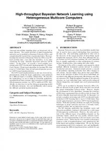
Figure 1: Example of a BN for medical diagnosis. Rectangles represent discrete random variables and ovals represent continuous random variables.
5
Some of the earliest work on BNs, and one of the motivations for the notion, was to add probabilities to expert systems used for medical diagnosis. The Quick Medical Reference Decision Theoretic (QMR-DT) project [25] is building a very large (448 nodes and 908 edges) BN. Consider, for example, the BN shown in Figure 1. The BN is a very small diagnostic BN which specifies a stochastic model with four random variables: 1. Flu, meaning that a patient has influenza. 2. Cold, meaning that a patient has one of a number of milder respiratory infections. 3. Perceives Fever, meaning that the patient perceives that he/she has a fever. 4. Temperature, the continuous random variable representing a measurement of the patient’s body temperature. Note that three of the random variables are Boolean, the simplest kind of discrete random variable, and that the fourth random variable is continuous. Two of the nodes have no incoming edges, so their CPDs are just PDs, and because the nodes are Boolean, they can be specified with just one probability. We assume that P r(F lu) = 0.0001 and that P r(Cold) = 0.01, reflecting the fact that influenza is far less common than the common cold. The CPD for the Perceives Fever (PF) node has two incoming edges, so its CPD is a table that gives a conditional probability for every combination of inputs and outputs. For example, this CPD might be the following: Table 1 not(PF) not(Flu) and not(Cold) 0.99 not(Flu) and (Cold) 0.90 (Flu) and not(Cold) 0.10 (Flu) and (Cold) 0.05
PF 0.01 0.10 0.90 0.95
The CPD for the Temperature (T) node has two incoming edges, so its CPD will have 4 entries as in the case above, but because T is continuous, it must be specified using some technique other than a table. For example, one could model it as a normal distribution for each of the 4 cases as follows: Table 2 Mean not(Flu) and not(Cold) 37.0 not(Flu) and (Cold) 37.5 (Flu) and not(Cold) 39.0 (Flu) and (Cold) 39.2 6
Std Dev 0.5 1.0 1.5 1.6
As an example of one term of the JPD, consider the probability of the event (F lu) ∩ not (Cold) ∩ (P F ) ∩ (T ≤ 39.0). This will be the product: P r(F lu)(1 − P r(Cold))P r(P F | F lu and not Cold)P r(T ≤ 39.0 | F lu and not Cold) which is the product (0.0001)(.99)(.90)(0.5) = 0.004455. Although the BN example above has no directed cycles, it does have undirected cycles. It is much harder to process BNs that have undirected cycles than those that do not. Some BN tools do not allow undirected cycles because of this. Many of the classical stochastic models are special cases of this general graphical model formalism. Although this formalism goes by the name of Bayesian network, it is a general framework for specifying JPDs, and it need not involve any applications of Bayes’ law. Bayes’ law becomes important only when one performs inference in a BN, as discussed below. Examples of the classical models subsumed by Bayesian networks include mixture models, factor analysis, hidden Markov models, Kalman filters and Ising models to name a few. BNs have a number of other names. One of these, belief networks, happens to have the same acronym. BNs are also called probabilistic networks, directed graphical models, causal networks and “generative” models. The last two of these names arise from the fact that the edges can be interpreted as specifying how causes generate effects. One of the motivations for introducing BNs was to give a solid mathematical foundation for the notion of causality. In particular, the concern was to distinguish causality from correlation. A number of books have appeared that deal with these issues such as one by Pearl [40] who originated the notion of BNs. For causation in biology see [43]. Other books that deal with this subject are [13, 46].
2.3
Stochastic Inference
Having defined the notion of a BN, a number of issues immediately arise: 1. How does one construct a BN? 2. Having constructed a BN, what does one do with it? The first question will be the subject of Section 4. We now consider the second question. Having found a BN, one can perform inference with it. A BN, in fact, acts something like a rule engine. In a rule engine, one specifies a collection of if-then rules, called the rule base. One can then input a collection of known facts (typically obtained by some kind of measurement or observation). The rule engine then explicitly (as in a forward chaining rule engine) or implicitly (as in a backward chaining rule engine) infers other facts using the rules. The set of specified and inferred facts form the knowledge base. One can then query the knowledge base concerning whether a particular fact or set of facts has been inferred. 7
As in a rule engine, one can specify known facts to a BN (via measurement or observation), and then query the BN to determine inferred facts. Specifying known facts is done by giving the values of some of the random variables. The values can be given as actual crisp values or as probability distribution on the values. These nodes that have been given values are termed the evidence. One can then choose one or more of the other nodes as the query nodes. The answer to the query is the JPD of the query nodes given the evidence. Consider first the case of inference with no evidence at all. In this case, the probability distribution of the query nodes is computed by summing the terms of the JPD over all of the random variables that are not in the query set. For continuous random variables, one must integrate over the probability density. Consider the diagnostic BN in Figure 1. Suppose we would like to know the probability that a patient reports a fever. Integrating over the temperature node produces this JPD (rounding all results to 4 decimal places): Table 3 Event A not(Flu) and not(Cold) not(Flu) and (Cold) (Flu) and not(Cold) (Flu) and (Cold)
Pr(PF and A) Pr(not(PF) and A) (0.9999)(0.99)(0.01) = 0.0099 (0.9999)(0.99)(0.99) = 0.9800 (0.9999)(0.01)(0.10) = 0.0010 (0.9999)(0.01)(0.90) = 0.0090 (0.0001)(0.99)(0.90) = 0.0001 (0.0001)(0.99)(0.10) = 0.0000 (0.0001)(0.01)(0.95) = 0.0000 (0.0001)(0.01)(0.05) = 0.0000
Next, by summing the columns, one obtains the distribution of the PF node (except for some roundoff error): P r(P F ) = 0.011, P r(not(P F )) = 0.989 The process of summing over random variables is called marginalization, or computing the marginal.
Figure 2: Example of diagnostic inference using a BN. The evidence for diagnosis is the perception of a fever by the patient. The question to be answered is whether the patient has influenza. Now suppose that we have some evidence, say that the patient is complaining of a fever, and that we would like to know whether the patient has influenza. This is shown in Figure 2. The evidence presented to the BN is the fact that the random variable PF is true. The query is the value of the Flu random variable. The evidence is asserted by conditioning on the evidence. This is where Bayes’ law finally appears and is the reason why BNs are 8
named after Bayes. To compute this distribution, one first selects the terms of the JPD that satisfy the evidence, compute the marginal distribution, and finally normalize to get a probability distribution. This last step is equivalent to dividing by the probability of the evidence. To see why this is equivalent to Bayes’ law, consider the case of two Boolean random variables A and B joined by an edge from A to B. The probability distribution of a Boolean random variable is determined by just one probability, so it is essentially the same as an event. Let A and B be the two events in this case. The BN is specified by giving P r(A), P r(B | A) and P r(B | not A). Suppose that one is given the evidence that B is true. What is the probability that A is true? In other words, what is P r(A | B)? The JPD of this BN is given by the four products P r(B | A)P r(A), P r(not B | A)P r(A), P r(B | not A)P r(not A), and P r(not B | not A)P r(not A). Selecting just the ones for which B is true, gives the two probabilities P r(B | A)P r(A) and P r(B | not A)P r(not A). The sum of these two probabilities is easily seen to be P r(B). Dividing by P r(B) normalizes the distribution. In particular, P r(A | B) = P r(B | A)P r(A)/P r(B), which is exactly the classical Bayes’ law. Returning to the problem of determining the probability of influenza, the evidence requires that we select only the terms of the JPD for which PF is true, then compute the marginal. Integrating over the temperature results in the first column of Table 3 which is the following: Table 4 Event A Pr(PF and A) not(Flu) and not(Cold) (0.9999)(0.99)(0.01) = 0.0099 not(Flu) and (Cold) (0.9999)(0.01)(0.10) = 0.0010 (Flu) and not(Cold) (0.0001)(0.99)(0.90) = 0.0001 (Flu) and (Cold) (0.0001)(0.01)(0.95) = 0.0000 We are only interested in the Flu node, so we sum the rows above in pairs to get: Table 5 Event A Pr(PF and A) not(Flu) 0.0109 (Flu) 0.0001 Normalizing gives P r(F lu) = 0.009. Thus there is less than a 1% chance of having the flu even if one is complaining of a fever. This increases the probability of having the flu substantially over the case of no evidence, but it is still relatively low. The most general form of BN inference is to give evidence in the form of a probability distribution on the evidence nodes. The only difference in the computation is that instead of selecting the terms of the JPD that satisfy the evidence, one multiplies the terms by the probability that the evidential event has occurred. In effect, one is weighting the terms by 9
the evidence. We leave it as an exercise to compute the probability of the flu as well as the probability of a cold given only that there is a 30% chance of the patient complaining of a fever. BN inference is substantially more complex when the evidence involves a continuous random variable. We will consider this problem later. Not surprisingly, many BN tools are limited to discrete random variables because of this added complexity. In principle, there is nothing special about any particular node in the process of BN inference. Once one has the JPD, one can assert evidence on any nodes and compute the marginal distribution of any other nodes. However, BN algorithms can take advantage of the structure of the BN to compute the answer more efficiently. As a result, the pattern of inference does affect performance in practice. The various types of inference are shown in Figure 3. Generally speaking, it is easier to infer in the direction of the edges of the BN than against them. Inferring in the direction of the edges is called causal inference. Inferring against the direction of the edges is called diagnostic inference. Other forms of inference are called mixed inference.
Figure 3: Various types of inference. Although information about any of the nodes (random variables) can be used as evidence, and any nodes can be queried, the pattern of inference determines the computational complexity for obtaining inferred probability distribution. So far we have considered only discrete nodes. Continuous nodes add some additional complexity to the process. There are several ways to deal with such nodes: 1. Discretize. The possible values are partitioned into a series of intervals, and one only considers which interval occurs. This has the disadvantage that it reduces the accuracy of the answer. However, it has the advantage that one only has to deal with discrete nodes. Many BN tools (such as MSBNx [26]) can only deal with discrete random variables, and one must discretize all continuous random variables to use such tools. 2. Restrict to one class of distributions. A common restriction is to use only normal (Gaussian) distributions. This choice is supported by the central limit theorem. As in the case of discretization, it reduces the accuracy of the answer. (In fact, discretization is a special case of this assumption.) The advantage of this assumption 10
is that the number of parameters needed to specify a distribution can be reduced dramatically. In the case of (single-variable) normal distributions, one needs only two parameters. There are many other choices for class of distribution that can be used. There will always be a trade-off between improved accuracy versus the increase in computational complexity. Since there will be many sources of error over which one has no control, the improvement in accuracy resulting from a more complex class of distribution may not actually improve the accuracy of the BN. 3. Use analytic techniques. This is more a theoretical than a practical approach. Only very small BNs can be processed this way, and it is difficult to automate. Furthermore, the comment above about sources of error over which one has no control also applies here. The techniques above are concerned with the specification of PDs. A CPD is a function from the possible values of the parent nodes to PDs on the node. If there are only a few possible values of the parent nodes (as in the diagnostic example in Figure 1), then explicitly listing all of the PDs is feasible. Many BN tools have no other mechanism for specifying CPDs. When the number of possible values of the parent nodes is large or even infinite, then the CPD may be much better specified using an analytic function. In the infinite case, one must use this technique. Curve fitting techniques such as least squares analysis can be used to choose the analytic function based on the available data. A BN with both discrete and continuous nodes is called a hybrid BN. The diagnostic BN example above is a hybrid BN. When continuous nodes are dependent on discrete nodes, inference will produce a compound (mixed) Gaussian distribution. Such a distribution is the result of a compound process in which one of a finite set of Gaussians is selected according to a probability distribution, and then a value is chosen based on the particular Gaussian that was selected. Compound Gaussians are harder to deal with than simple Gaussians, so it is common to merge (or fuse) the mixture to a single Gaussian. This is discussed in Section 3.2. If a discrete node is dependent on continuous nodes, then the discrete node can be regarded as forming a classifier since it takes continuous inputs and produces a discrete output which classifies the inputs. The CPDs for this situation are usually chosen to be logistic/softmax distributions. Connectionist (also called neural) networks are an example of this. BNs are not the only graphical representation for stochastic models. Undirected graphical models, also called Markov Random Fields (MRFs) or Markov networks, are also used, especially in the Physics and vision communities. One application of BNs is to assist in decision making. To make a decision based on evidence one must quantify the risk associated with the various choices. This is done by using a utility function. It is possible to model some utility functions by adding value nodes (also called utility nodes to a BN and linking them with dependency edges to ordinary BN nodes and to other utility nodes. The result of a decision is an action that is performed, and these can also be represented graphically by adding decision nodes and edges to a BN 11
augmented with utility nodes. A BN augmented with utility and action nodes is called an influence diagram (also called a relevance diagram) [22]. An influence diagram can, in principle, be used to determine the optimal actions to perform so as to maximize expected utility.
2.4
Dynamic and Evolving Bayesian Networks
BNs can be dynamic in several very different ways: 1. The BN can represent stochastic processes that vary in time. BNs generalize stochastic dynamic systems, in general, and hidden Markov models in particular. However, the BN structure (including both the CPDs and the graph) do not vary. 2. The probabilistic structure of the BN could vary in time. In other words, the entries in the CPDs could change, but the BN graph does not. 3. The BN graph could vary in time by changing the set of nodes as well as the set of edges. This is the most extreme kind of variation. Of these three kinds of dynamic BN, only the first is normally given the name dynamic Bayesian network and the acronym DBN. Consequently some other name must be used for a BN that truly varies in time. We will call it an evolving Bayesian network.
Figure 4: A Dynamic Bayesian Network. Each column represents one point in time (a “time slice”). A DBN is modeled by repeating the BN once for each “time slice”. An example of a 3-node DBN is shown in Figure 4. Each node is duplicated in each time slice. The nodes that specify the dynamics have the property that each copy of the node in one time slice is dependent on one or more nodes in the previous time slice. The structure of the DBN is exactly the same in each time slice. Furthermore, the CPDs specifying the dependencies between time slices are the same for every time slice. 12
An evolving DBN can change by modifying CPDs without changing the structure of the dependencies. This is shown in Figure 5. The changes to the CPDs can be obtained using incremental versions of the same techniques that are used for constructing the original CPD. These are discussed in Section 3.1 below.
Figure 5: An Evolving Bayesian Network in which a CPD has changed. It is also possible for the dependencies to change. In Figure 6, the BN has acquired a new node and edge. As a result it also now has an additional CPD. This CPD can be obtained from an already known template using the techniques discussed in Section 4.2. The CPD may subsequently evolve as discussed above. Allowing BNs to evolve is important when one is modeling situations. Awareness of the current situation is essential in complex tasks such as coordinating responses to an emergency (e.g., extreme weather, accidents, fires and terrorist acts). In addition to the uncertainties involved in such situations, they also evolve, sometimes quite rapidly.
Figure 6: An Evolving Bayesian Network which as acquired a new node. One important requirement for situation awareness is to be aware of the relevant entities in the region of interest as well as their characteristics. However, this alone is not sufficient for one to have situation awareness. One must also understand the relationships between the entities. This makes situation awareness especially difficult because of the large number of potential relationships between entities. Situation awareness was originally concerned with human situation awareness, and research in this area focused on improving the human-computer interface to assist the human in achieving situation awareness [9]. However, more recently situation awareness is being studied as a form of data fusion based on ontologies and logical inference. A core ontology for situation awareness has been formalized [4, 34], and techniques have been developed for propagating uncertainty in situations using fuzzy logic [34] as well as using BNs [28]. 13
2.5
Exercises
1. In the diagnostic BN in Figure 1, one can use either a temperature measurement or a patient’s perception of a fever to diagnose influenza. Although these two measurements are a priori independent, they become dependent when one observes that the patient has the flu or a cold. In statistics this is known as Berkson’s paradox, or “selection bias.” It has the effect that a high temperature can reduce the likelihood that a patient reports being feverish and vice versa. Compute the JPD of the PF and T nodes in this BN given the observation that the patient has influenza. 2. Compute the probability that a patient has influenza using temperature measurements. For example, try 37, 38, 39 and 40 degrees. These are all (in theory) exact measurements. In fact, a thermometer, like all sensors, can only give a measurement that is itself a random variable. Compute the probability of influenza given a temperature of 38.40 degrees, normally distributed with standard deviation 0.20 degrees.
3
Constructing Bayesian Networks
This section gives some background on current statistical methods for constructing and evaluating probability distributions. It begins with an overview of techniques for empirically determining PDs, CPDs and BNs from data. Such data is regarded as being used to “train” the probabilistic model, so the techniques are known as machine learning methods. In Section 3.2 a somewhat different point of view is taken in which information of various kinds is combined or “fused”. Although these techniques are closely related to machine learning, they are known as data fusion methods. Issues related to evaluation and testing of BNs are discussed in Section 3.3, and this part of the paper ends in Section 3.4 by considering the problem of representing BNs as well as the relationship between BNs and ontologies.
3.1
Machine Learning
This is a very large area that would be difficult to survey adequately, so we give only an overview. Since a BN is just a way of representing a JPD, virtually any data mining technique qualifies as a mechanism for constructing a BN. It is just a matter of expressing the end result as a BN. For example, one might be interested in the body mass index (BMI) of individuals in a research study. The individuals have various characteristics, such as sex and age. Computing the average BMI of individuals with respect to these two characteristics gives rise to a three-node BN as in Figure 7. The CPD for the BMI node gives the mean and standard deviation of the BMI for each possible combination of sex and age in the study.
14
Figure 7: Bayesian network for the result of a research study of body mass index as a function of age and sex. It is common to assume that the CPDs are independent of each other, so they can be estimated individually. When data for both the parent nodes and the child node are available, estimating the CPD reduces to the problem of estimating a set of PDs, one for each of the possible values of the parent nodes. There are many techniques for estimating PDs in the literature. They can be classified into two categories: 1. Frequentist methods. These methods are associated with the statistician and geneticist Ronald Fisher, and so one sometimes sees at least some of these methods referred to as Fisherian. They also go by the name maximum likelihood (ML) estimation. The CPDs of discrete nodes that are dependent only on discrete nodes are obtained by simply counting the number of cases in each slot of the CPD table. This is why these techniques are called “frequentist”. The CPDs for Gaussian nodes are computed by using means and variances. Other kinds of continuous random variable are computed using the ML estimators for their parameters. 2. Bayesian methods. These methods also go by the name maximum a posteriori (MAP) estimation. To perform such an estimation, one begins with a prior PD, and then modifies it using the data and Bayes’ law. This is a special case of a more general process, discussed in Section 3.2, whereby known CPDs can be improved by using additional data or by using other BNs. The use of an arbitrary prior PD makes these methods controversial. However, one can argue that (in most cases) the ML technique is just the special case of MAP for which the prior PD is the uniform distribution. In other words, the prior PD is the one which represents the maximum amount of ignorance possible. However, the uniform distribution does not always exist, and when it does, there can be several choices for it. So one is making an arbitrary choice even in for the ML technique. If one has some prior knowledge, even if it is subjective, it is helpful to include it in the estimation. As the amount of data and learning increase, the effect of the prior PD gradually disappears. The estimation techniques discussed above assume that data about all of the relevant nodes was available. This is not always the case. When one or more node is not directly 15
measurable, one can either remove it from the BN (as discussed in Section 4.5) or attempt to estimate it indirectly. The latter can be done by using BN inference iteratively. One treats the unobservable nodes as query nodes and the observable nodes as evidence nodes in a BN inference process. One then computes the expectations of the unobservable nodes and uses these values as if they were actually observed. One can then use ML or MAP as above. This whole process is then repeated until it converges. This technique is known as Expectation Maximization (EM). It is possible to use learning techniques to learn the structure of the BN graph as well as the CPDs. These tend to have very high computational complexity, so they can only be used for small BNs. In practice, it is much better to start with a carefully designed BN and then modify it in response to an evaluation of the quality of its results. Connectionist networks are a class of BNs that are designed for efficient machine learning. Such BNs are most commonly known as “neural networks” because they have a superficial resemblance to the networks of neurons found in vertebrates, even though neurons have very different behavior than the nodes in connectionist networks. Many kinds of connectionist network support incremental machine learning. In other words, they continually learn as new training data is made available. In other words, they are evolving BNs as discussed in Section 2.4, an example of which is shown in Figure 5. For example, in the diagnostic BN in Figure 1, some of the patients may be tested for influenza using a more accurate (but more expensive) flu test. This information could be used to improve the CPD entries. Connectionist networks constitute a large research area, and there are many software tools available that support them. There is an extensive FAQ for neural networks including lists of both commercial and free software [42]. Although connectionist networks are a special kind of BN, the specification of a connectionist network is very different from the specification of a BN. As a result, the results for connectionist networks may not apply directly to BNs or vice versa. However, BNs are being used for connectionist networks [33] and some connectionist network structures are being incorporated into BNs as in [36].
3.2
Information Fusion
Stochastic models are a versatile language for expressing any kind of uncertainty. Measurements are intrinsically uncertain, and the uncertainty of measurements by instruments (such as sensors) are very well understood. When multiple sensors of various types have overlapping ranges, it is necessary to combine their measurements. The process of seamlessly integrating data from disparate sources is most commonly called data fusion, although it has also been called reconciliation. Although multisensor data fusion originated in military applications, the techniques are now also being used in many other applications. Data fusion is especially important for situation awareness. In fact, in the standard architecture for data fusion [47], situation awareness is one of the levels of data fusion. Measurement uncertainty and data fusion have been recognized as being an important BN design patterns [37]. However, this is not the same as deriving CPDs using data fusion. 16
While this should, in principle, be an effective method for deriving BNs, it must be done with considerable care, as has been shown in [8].
3.3
Evaluation and Validation
Testing and validation have always been accepted as an important part of any development activity. This is especially true for BN development. BNs have the advantage that there is a well-developed, sophisticated mechanism for testing hypotheses about probability distributions. However, this is also a disadvantage because statistical hypothesis testing generally requires more than one test case, and even with a large sample of test cases the result can be equivocal. A BN test case is usually a specific example of a stochastic inference. As is the case with software engineering, constructing enough test cases to handle all of the possibilities that can occur can be difficult or impossible. This is especially true for large systems. Furthermore, BN development efforts usually have no precisely stated purpose. As a result, one cannot formally test that the purpose has been achieved. There are several ways to deal with validating BNs: 1. Sensitivity analysis. This technique determines the impact of inaccuracies of the CPD entries by systematically varying them and recording the effects on test cases. As one might expect, different CPD entries of BNs can have very different sensitivities [21, 41]. Aside from being useful for testing, sensitivity analysis can be used during development by using it to focus attention on the probabilities that need to be determined more accurately. 2. Uncertainty analysis. In this technique, all of the probabilities are varied simultaneously by choosing each one from a prespecified distribution that reflects their uncertainties. One then records the effects on test cases. This technique can determine the overall reliability of a BN. However, it yields less insight into the effect of separate probabilities than is the case for sensitivity analysis. 3. Unit testing. Smaller systems are much easier to test. Unfortunately, it is difficult to separate the effects of one part of a BN from another. Sensitivity analysis attempts to localize effects, but it is not a true unit test technique because the part of the BN being tested is not isolated from the rest of the BN. With all current BN tools, one can only test individual nodes or the entire BN: there are no intermediate internal structures that can be tested independently. The notions of OONF and OOBN should make it possible to perform meaningful unit testing, but few current tools support these notions. 4. One activity that can be performed without explicitly specifying requirements is formal consistency checking. With current BN tools, there is only one axiom that one can check: the BN must be acyclic. OOBNs add the possibility of performing 17
type-checking, and this is valuable, but it is still only syntactic. There is not yet a notion of semantic consistency for BNs. For example, are there analogs of the software concepts of pre-conditions and post-conditions? 5. In the absence of explicitly stated requirements, the only alternative is to involve the stakeholders directly in the testing process. Testing would proceed by presenting a stakeholder or group of stakeholders with randomly generated scenarios designed to determine the accuracy of the ontology.
3.4
Ontologies to Represent Bayesian Networks
An ontology is fundamentally a language for expressing concepts in a domain. One could, in particular, use ontologies to represent BNs. There already exists an format for representing BNs, called the XML Belief Network format (XBN) [48]. This XML file format was developed by Microsoft’s Decision Theory and Adaptive Systems Group. This format evolved from a standardization effort to develop the Bayesian Network Interchange Format (BNIF). In the XBN format, a node is defined using a VAR element. The values that a node can take are called states and they are specified using STATENAME elements. The directed edges are specified using ARC elements. The CPD table for one node is specified using a DIST element. A particular CPD for a choice of parent values is represented using a DPI element. The XBN format does not support continuous random variables. So to represent a BN that has such nodes it is necessary to extend the format. To represent the BN in Figure 1, we added two attributes to the DPI element (the MEAN and VARIANCE of the distribution). Here is what this BN looks like in terms of the XBN format: Patient has influenza Absent Present Patient has mild upper respiratory
18
viral infection Absent Present Patient self-diagnoses a fever Absent Present Oral measurement of the body temperature of the patient 0.9999 0.0001 0.99 0.01 0.99 0.01 0.90 0.10 0.10 0.90 0.05 0.95
19
The scientific research literature is a huge repository of knowledge about the natural universe. Representation languages have been developed for some parts of this literature. For example, there has been extensive work on representing, querying and inferring from experimental procedures (usually called “Materials and Methods”) [2, 3, 14, 15, 12, 16, 10]. Most of the scientific research literature includes probabilistic information. The results of experiments, for example, can be expressed as a stochastic model. Thus a complete specification of an experiment, including both how it was conducted and what resulted from it, requires an ontology that includes both procedural information and BNs. Techniques have been developed for extracting Materials and Methods information (cf., the citations above), but there are not yet techniques for extracting the results of the experiments.
4
Software Development Techniques for Bayesian Networks
We now consider the important question of how to construct BNs and compare the development of BNs with the development of software. While there are many tools for performing inference in BNs, the methodology commonly employed for developing BNs is rudimentary. A typical methodology looks something like this: 1. Select the important variables. 2. Specify the dependencies. 3. Specify the CPDs. 20
4. Evaluate. 5. Iterate over the steps above. Furthermore, the first three steps are usually performed by eliciting the information from experts. As a result the BNs can be highly subjective. In principle, the evaluation phase should be able to deal with this, but that is analogous to producing software by iterating the loop of programming (without any explicit requirements or design) and testing. This simple methodology will work for relatively small BNs, but as in the case of software, it does not scale up to the larger BNs that are now being developed. Consequently, methodologies and processes for BN development have been developed, usually by adapting software engineering methodologies and processes. The following are some of the software development techniques that can be used as part of the process of constructing BNs, and each of them is discussed in more detail in its own section: 1. Systematic requirements engineering. Without clearly stated requirements, it is difficult to determine whether a BN has been successfully developed. 2. Ontologies. Although ontologies are emerging as an important tool for dealing with some important issues facing information processing, no ontological framework for BNs has been proposed that would use the ontology for more than just background and documentation. 3. Design patterns. This is a popular technique in software engineering, and they have also been used in BN network development. A BN development methodology has been introduced in [37] that is based on design patterns. 4. Refactoring. A BN can be improved by adjusting its structure. Unlike refactoring in software, the consequences of such modifications are usually not obvious. Substantial software assistance is necessary to support this mechanism. A BN development process has been introduced in [29] that is based primarily on refactoring. 5. Object-oriented and component-based techniques. These have only recently been successfully introduced to the field of BNs in [28]. However, there is much more that needs to be done. All of these techniques show promise for assisting in BN development. However, all of them are being applied more by analogy than by direct integration.
4.1
Requirements Engineering
Modern software development process models include a requirements phase, and there is a substantial literature on this subject, including a journal exclusively devoted to it [32]. This activity involves domain experts (also known as subject matter experts or SMEs). 21
Current BN development also employs SMEs. In fact, most of the development can be attributable to the judgments and expertise of the SMEs. Consequently SMEs are involved throughout the development process. While SMEs are involved in both requirements analysis and knowledge acquisition, their role is very different in the two cases. Requirements analysis not only involves acquiring an understanding of the domain, it also determines the required function, performance, behavior, and interfaces. BN development typically omits these latter requirements. Indeed, the notion of an BN interface is only now beginning to be understood (cf., [28, 27]). In most cases, BN development projects have no explicitly stated purpose, no separate requirements phase and no requirements document. When there is a stated purpose, it is usually too generic to be useful in the development process. Having a detailed stated purpose would not entirely determine the required function, performance, behavior and interfaces, but it would certainly help. Because the amount of knowledge to be acquired may be very large, it is important for the knowledge to be structured. It is also important to track the source of knowledge so that one can determine its trustworthiness. These issues can be addressed to some degree by using ontologies (see Section 4.5 above). Of course, ontologies should also be developed using a well structured methodology as was discussed in [1].
4.2
Object-Oriented Techniques
Object-oriented (OO) techniques offer several possible advantages. The first is the possibility of a more systematic design phase in BN development. Another advantage is that using an OO design might be able to improve performance. A notion of object-oriented BN (OOBN) was introduced in [28] that shows considerable promise as the basis for using OO techniques in BN development. The basic OOBN concept is called an “object” which is similar in many ways to the notion of object in object-oriented systems. An OOBN object can be just a random variable, but it can also have a more complex structure via attributes whose values are other objects. An OOBN object can correspond to an entity or it can be a relationship between entities. A simple OOBN object corresponds to a BN node. It has a set of input attributes (i.e., the parent nodes in the BN) and an output attribute (i.e., its value). A complex OOBN object has input attributes just as in the case of a simple OOBN object, but a complex object can have more than one output attribute. It can also have encapsulated attributes that are not visible outside the object. A complex object corresponds to several BN nodes, one for each of the outputs and encapsulated attributes. In principle, the notion of a complex object is just a mechanism for grouping nodes in a BN. The JPD and the process of inference are exactly the same whether or not the grouping is used. However, by grouping (encapsulating) nodes into objects, one gains a number of significant advantages: 1. Complex objects can be assigned to classes which can share CPDs. By reusing CPDs, this greatly simplifies the task of specifying a BN. 22
2. The complex objects have an interface which can be used for validating the BN. This is similar to type-checking in OO languages. 3. Classes can inherit from other classes which allows for still more possibilities for reuse. 4. Encapsulation can be used during inference to improve performance. This advantage is especially compelling. As shown in [28], if a BN has an OO structure, then the performance of inferencing can be improved by an order of magnitude or more compared with even a well optimized BN inference algorithm. Another development feature of OOBNs is the notion of an object-oriented network fragment (OONF). An OONF is a generalization of a BN which specifies the conditional distribution of a set of value attributes given some set of input attributes. If there are no input attributes, then an OONF is a BN. An OONF can be defined recursively in terms of other OONFs, An OONF can also be used as a component which can be “reused” multiple times in a single BN. For example, one can use OONF to introduce the OO concept of a class to BNs. Component-based methods are a powerful development methodology that allow one to build BNs from standard components that have been constructed independently. While the notions of OONF and OOBN show great promise as a BN development methodology, they do not integrate BNs with software development. The OO techniques used in OOBNs are by analogy only.
4.3
Ontologies as Bayesian Networks
Ontologies are emerging as an important tool for dealing with some of the most important issues facing information processing: 1. Ever larger amounts of data are available at much faster rates. 2. Data structures are increasing in their complexity. 3. Much more diverse sources of information are becoming relevant to each activity. These trends have also increased interest in automating many activities that were traditionally performed manually. Web-enabled agents represent one technology for addressing this need [35]. These agents can reason about knowledge and can dynamically integrate services at run-time. Formal ontologies are the basis for such agents. The Resource Description Framework (RDF) [30] and the Web Ontology Language (OWL) [44] are ontology language standards developed under the auspices of the World Wide Web Consortium. RDF is the basic language with the minimum number of constructs necessary for expressing ontologies. OWL adds features to RDF in a series of three versions (or levels), called OWL Lite, OWL-DL and OWL Full. The distinctions between RDF and OWL and among the three OWL levels are explained in [50]. 23
The DL in OWL-DL stands for “description logic”. This is a form of logic that class construction as the primary modeling mechanism. A class is essentially the same as the notion of set in mathematics. A class is constructed by specifying its members using other classes. For example, the definition of autoradiography is “A technique that uses X-ray film to locate radioactively labeled molecules or fragments of molecules.” From a DL perspective, autoradiography is a class consisting of those members of the technique class that use X-ray film to locate radioactively labeled molecules or fragments of molecules. Queries to an OWL-DL ontology would mostly be concerned with whether or not a specific entity belongs to a specified class. Expressing BNs using richer ontology languages, such as RDF or OWL, would be beneficial for a number of reasons. 1. One can take advantage of language constructs that exist in RDF and OWL that cannot be expressed in XML alone. 2. RDF and OWL have inferencing capabilities that XML does not have. 3. A rules language is being developed for OWL. If BNs were expressed using OWL, then it should be possible to specify both crisp, logical rules and fuzzy, probabilistic rules in the same document. 4. The BN can be annotated with additional information integrating it with other kinds of information. One of the earliest large BNs was the QMR-DT mentioned in Section 2 which added probabilities to an expert system. The close connection between expert systems and ontologies would suggest that it ought to be possible to “add probabilities” to ontologies. Perhaps because of this analogy, an active research area has developed that is attempting to do this for ontologies, especially for ontologies based on description logic. See [7, 27]. Given an OWL-DL ontology, the corresponding BN has one node for each class. This node is a Boolean random variable which is true if and only if an entity belongs to the class. Relationships between classes give rise to edges between the nodes of the classes. The most common relationship is the subclass relationship which means that one class is contained in another. Obviously this will result in a stochastic dependency. Other kinds of relationship can be expressed in terms of classes. For example, the age of a person (in years) gives rise to a collection of disjoint subclasses of the person class, one for each possible value of the age of a person. Although this technique does seem to be a natural way to “add probabilities” to ontologies, it does not seem to produce BNs that are especially useful. The most peculiar feature of these BNs is that all of the classes are ultimately subclasses of a single universal class (called the Thing class), and the random variable for a class represents the probability that a randomly chosen thing is a member of the class. While this might make sense for some class hierarchies, the hierarchies of ontologies often contain a wide variety of types of entity. For example, a biomedical ontology would contain classes for research papers, 24
journals, lists of authors, drugs, addresses of institutions, etc. It is hard to see what kind of experiment would sometimes produce a drug, other times produce a list of authors and still other times produce an address. On the other hand, this technique can be the starting point for BN development, especially for diagnostic BNs. An example of this is discussed in Section 4.5, where the ontology is used as the background for the development of a BN. The disadvantage of using ontologies this way is that whatever formal connection exists between the ontology and the BN is quickly lost as the BN is modified. As a result, one cannot use any logical consequences entailed by the ontology during BN inference. Indeed, the ontology ultimately furnishes no more than informal documentation for the BN.
4.4
Design Patterns
Design patterns for BNs were introduced by [37], where they were called “idioms.” Five idioms were identified by [37]: 1. Definitional/Synthesis. This pattern models the synthesis or combination of many nodes into one node. It also models deterministic definitions. 2. Cause-Consequence. This models an uncertain causal process whose consequences are observable. 3. Measurement. This models the uncertainty of a measuring instrument. 4. Induction. This models inductive reasoning based on populations of similar or exchangeable members. 5. Reconciliation. This models the reconciliation (also called fusion) of results from competing sources. Other authors have mentioned patterns that may be regarded as being design patterns, but in a much more informal manner. For example in [36] quite a variety of patterns are shown such as the DBMs reproduced in Figure 8. In each of the patterns, the rectangles represent discrete nodes and the ovals represent Gaussian nodes. The shaded nodes are visible (observable) while the unshaded nodes are hidden. Inference typically involves specifying some (or all) of the visible nodes and querying some (or all) of the hidden nodes.
4.5
Refactoring
In a series of articles Helsper and van der Gaag [17, 20, 18, 19] are developing a methodology for BN development that uses ontologies. The authors have studied the use of their methodology within the domain of oesophageal cancer.
25
Figure 8: Various informal patterns for DBNs. These examples are taken from [36]. The Helsper methodology uses ontologies more as a background for the design process than as a formal specification for the BN structure. This is in contrast with the OOBN technique in Section 4.2 in which the object-oriented design specifies not only the BN completely but it is also used in the inference algorithm. In the Helsper methodology the ontology is used to provide an initial design for the BN in a manner similar to the way that this is done in Section 4.3. This step in the methodology is called translating. However, this initial design is modified in a series of steps based on domain knowledge. Some of this is available in the ontology but most of it must be elicited from domain experts. The ontology “serves to document the elicited domain knowledge.” The purpose and requirements of the BN are also important, but it is not clear whether the Helsper methodology has a separate requirements phase. What makes the Helsper-van der Gaag methodology interesting is the systematic modification techniques that are employed. The methodology refers to this phase as improving and optimizing. The modifications must follow a set of guidelines, but these guidelines are 26
only explained by examples in the articles. It appears that these modification techniques are similar to the refactoring that have been thoroughly described in software engineering. One example of a refactoring operation used by Helsper and van der Gaag is shown in Figure 9. In this operation, a node that depends on two (or more) other nodes is eliminated. This would be done if the node being eliminated is not observable or if it is difficult to observe the node. There are techniques for determining the CPDs for unobservable nodes such as the EM algorithm discussed in Section 3.1. However, this algorithm is time consuming. Furthermore, there is virtually no limit to what one could potentially model, as discussed in Section 2.1. One must make choices about what is variables are relevant, even when the could be observed, in order to make the model tractable.
Figure 9: Refactoring by eliminating a node that other nodes depend on. The result is that the parent nodes become dependent on each other. When a node is dependent on other nodes, the other nodes (which may otherwise be independent) become implicitly dependent on each other via the dependent node. In statistics this is known as Berkson’s paradox, or “selection bias.” The result of dropping a node is to make the parent nodes explicitly dependent on each other. This dependency can be specified in either direction, whichever is convenient and maintains the acyclicity of the BN. The refactoring operation shown in Figure 9 changes the JPD of the BN because one of the variables is being deleted. Furthermore, the new JPD need not be just the distribution obtained by marginalization to remove the deleted variable. At best, the new BN is a approximation to the marginalization of the original BN. It is a general fact that the direction of a directed edge in a BN is probabilistically arbitrary. If one knows the JPD of two random variables, then one can choose either one as the parent node and then compute the CPD for the child node by conditioning. In practice, of course, the specification works the other way: the JPD is determined by specifying the CPD. For a particular modeling problem, the direction of the edge will be usually be quite clear, especially when one is using a design pattern. However, sometimes the direction of the dependency is ambiguous, and one of the refactoring operations is to reverse the direction. In this case the JPD is not changed by the operation. This situation occurs, for example, when two variables are Boolean, and one of them subsumes the other. In other words, if one of the variables is true, then the other one is necessarily true also (but not vice versa). Suppose that X and Y are two Boolean random variables such that X implies Y. Then we know that P r(Y = true | X = true) = 1. 27
This gives one half of the CPD of one of the variables with respect to the other, and the dependency can go either way. This is shown in Figure 10
Figure 10: Refactoring by reversing the direction of a dependency when two Boolean nodes are related by subsumption.
5
Conclusion
This paper has presented the current state of the art in BN development methods. While these methods show great promise, many difficult challenges remain. Some of the major open problems of BN development are: 1. Better development methodologies. Some excellent progress has been made, but this problem remains open. This is especially true for dynamic and evolving BNs. 2. Better evaluation measures and methods. This is not just a question of better testing. It also requires better requirements gathering techniques so that one knows what is to be tested. 3. Closer connections with logic. The simple approaches that have been tried so far have not led to BNs that are very useful. Formal specifications of the rules for a BN to evolve promises a much deeper and more useful connection of logic and ontologies to BNs. 4. Better integration with dynamic systems. Classical dynamic systems can be expressed in terms of BNs. However, the structure of such BNs does not vary over time. Techniques for building and managing dynamically evolving BNs have yet to be developed. 5. Development of standard representations for interoperability. While there is an XML format for Bayesian networks, it is still rudimentary and has yet to be standardized. 6. Information fusion of BNs. This problem is also known as “reconciliation.” Fusion of probability distributions is well known and a very active area. However, it has yet to be extended to general BNs. 7. Natural language extraction of BNs. Extracting the BNs from scientific and engineering articles holds the potential for a considerably richer and deeper style of data mining from the literature. 28
Many techniques from software engineering, such as object-oriented techniques, ontologies, design patterns and refactoring, have analogs in BN development, and further elaboration of these analogies should help to meet these challenges. It is hoped that this paper will encourage further work in this area.
6
Acknowledgments
The author would like to thank the Division of Preventive Medicine of The Harvard Medical School for their support and encouragement. Any opinions, findings and conclusions or recommendations expressed in this material are those of the author(s) and do not necessarily reflect the views of Harvard University.
References [1] K. Baclawski. Ontology development. In International Workshop on Software Methodologies, Tools and Techniques, pages 3–26, 2003. Keynote address. [2] K. Baclawski, R. Futrelle, N. Fridman, and M. Pescitelli. Database techniques for biological materials & methods. In First Intern. Conf. Intell. Sys. Molecular Biology, pages 21–28, 1993. [3] K. Baclawski, R. Futrelle, C. Hafner, M. Pescitelli, N. Fridman, B. Li, and C. Zou. Data/knowledge bases for biological papers and techniques. In Proc. Sympos. Adv. Data Management for the Scientist and Engineer, pages 23–28, 1993. [4] K. Baclawski, M. Kokar, C. Matheus, J. Letkowski, and M. Malczewski. Formalization of situation awareness. In H. Kilov and K. Baclawski, editors, Practical Foundations of Behavioral Semantics, pages 25–40. Kluwer Academic Publishers, Dordrecht, The Netherlands, 2003. [5] B. Cukic et al. A bayesian approach to reliability prediction and assessment of component based systems. In Proc. of ISSRE, November 2001. [6] G. Dahll. Combining disparate sources of information in the safety assessment of softwarebased systems. Nuclear Eng. and Design, 195(3):307–319, 2000. [7] Z. Ding and Y. Peng. A probabilistic extension to ontology language OWL. In Proc. 37th Hawaii Intern. Conf. on Systems Science, 2004. [8] M. Druzdzel and F. D´iez. Criteria for combining knowledge from different sources in probabilistic models. J. of Machine Learning Research, 4:295–316, July 2003. [9] M. Endsley and D. Garland. Situation Awareness, Analysis and Measurement. Lawrence Erlbaum Associates, Publishers, Mahway, New Jersey, 2000.
29
[10] N. Fridman. Knowledge Representation for Intelligent Information Retrieval in Experimental Sciences. PhD thesis, College of Computer Science, Northeastern University, Boston, MA, 1997. [11] N. Friedman. Inferring cellular networks using probabilistic graphical models. Science, 303:799, February 6 2004. [12] R. Futrelle and N. Fridman. Principles and tools for authoring knowledge-rich documents. In DEXA 95 Workshop on Digital Libraries, pages 357–362, London, UK, 1995. [13] Glymour and Cooper, editors. Computation, Causation and Discovery. MIT Press, 1999. [14] C. Hafner, K. Baclawski, R. Futrelle, N. Fridman, and S. Sampath. Creating a knowledge base of biological research papers. In Proc. Second Intern. Conf. Intell. Sys. Molecular Biology, pages 147–155, 1994. [15] C. Hafner and N. Fridman. An ontology for substances and processes in Molecular Biology. In Proc. First International Summer Institute in Cognitive Science. Center for Cognitive Science, SUNY at Buffalo, Buffalo, NY, 1994. [16] C. Hafner and N. Fridman. Ontological foundations for biology knowledge models. In Proc. 4th International Conference on Intelligence Systems for Molecular Biology (ISMB96), pages 78–87. AAAI Press, Menlo Park, CA, 1996. [17] E. Helsper and L. van der Gaag. Ontologies for probabilistic networks: A case study in oesophageal cancer. In B. Kr¨ose, M. de Rijke, G. Schreiber, and M. van Someren, editors, Proc. 13th Belgium-Netherlands Conference on Artificial Intelligence, pages 125–132, Amsterdam, 2001. [18] E. Helsper and L. van der Gaag. Building bayesian networks through ontologies. In F. Harmelen van, editor, Proc. 15th European Conference on Artificial Intelligence, pages 680–684, Amsterdam, the Netherlands, 2002. [19] E. Helsper and L. van der Gaag. A case study in ontologies for probabilistic networks. In M. Bramer, F. Coenen, and A. Preece, editors, Research and Development in Intelligent Systems XVIII, pages 229–242. Springer-Verlag, London, England, 2002. [20] E. Helsper and L. van der Gaag. Experiences with modelling issues in building probabilistic networks. In A. Gomez-Perez and V. Benjamins, editors, Knowledge Engineering and Knowledge Management: Ontologies and the Semantic Web, Proceedings of EKAW 2002, pages 21–26, Berlin, Germany, 2002. [21] M. Henrion, M. Pradhan, B. del Favero, K. Huang, G. Provan, and P. O’Rorke. Why is diagnosis using belief networks insensitive to imprecision in probabilities? In Proc. 12th Conf. Uncertainty in Artificial Intelligence, pages 307–314, 1996. [22] R. Howard and J. Matheson. Influence diagrams. In R. Howard and J. Matheson, editors, Readings on the Principles and Applications of Decision Analysis, volume 2, pages 721–762. Strategic Decisions Group, Menlo Park, CA, 1981.
30
[23] B. Indurkhya. On the philosophical foundation of Lyee: Interaction theories and Lyee. In H. Fujita and P. Johannesson, editors, New Trends in Software Methodologies, Tools and Techniques, pages 45–51. IOS Press, Amsterdam, 2002. [24] B. Indurkhya. Some observations on the philosophical nature of software and their implications for requirement engineering. In H. Fujita and P. Johannesson, editors, New Trends in Software Methodologies, Tools and Techniques, pages 29–38. IOS Press, Amsterdam, 2003. [25] T. Jaakkola and M. Jordan. Variational probabilistic inference and the QMR-DT network. Journal of Artificial Intelligence Research, 10:291–322, 1999. [26] C. Kadie, D. Hovel, and E. Hovel. MSBNx: A component-centric toolkit for modeling and inference with bayesian networks. Technical Report MSR-TR-2001-67, Microsoft Research Technical Report, July 2001. [27] D. Koller, A. Levy, and A. Pfeffer. P-Classic: A tractable probabilistic description logic. In Proc. Fourteenth National Conf. on Artificial Intelligence, pages 390–397, Providence, RI, August 1997. [28] D. Koller and A. Pfeffer. Object-oriented bayesian networks. In Proc. Thirteenth Ann. Conf. on Uncertainty in Artificial Intelligence, pages 302–313, Providence, RI, August 1997. [29] K. Laskey and S. Mahoney. Network engineering for agile belief networks. IEEE Trans. Knowledge and Data Engineering, 12:487–498, 2000. [30] O. Lassila and R. Swick. Resource description framework (RDF) model and syntax specification, Feburary 1999. www.w3.org/TR/REC-rdf-syntax. [31] G. Leibniz. Monadology. In G.W. Leibniz Philosophical Texts (1714), pages 267–281. Oxford University Press, New York, 1998. Translated and edited by R. Woolhouse and R. Francks. [32] P. Loucopoulos and J. Mylopoulos, editors. Requirements Engineering. Springer-Verlag, Limited, London, 1996. [33] D. MacKay. Bayesian methods for neural networks - FAQ, 2004. www.inference.phy.cam.ac.uk/mackay/Bayes FAQ.html. [34] C. Matheus, M. Kokar, and K. Baclawski. A core ontology for situation awareness. In Proc. FUSION’03, July 2003. [35] D. McGuinness. Ontologies and online commerce. IEEE Intelligent Systems, 16(1):8–14, 2001. [36] Kevin Murphy. A Brief Introduction to Graphical Models and Bayesian Networks, 1998. www.ai.mit.edu/ murphyk/Bayes/bnintro.html. [37] M. Neil, N. Fenton, and L. Nielsen. Building large-scale Bayesian networks. The Knowledge Engineering Review, 15(3):257–284, 2000.
31
[38] G. Pai and J. Dugan. Enhancing software reliability estimation using bayesian networks and fault trees. Technical report, Department of ECE, The University of Virginia, VA, 22903, 1998. [39] J. Pearl. Graphical models for probabilistic and causal reasoning. In D. Gabbay and P. Smets, editors, Handbook of Defeasible Reasoning and Uncertainty Management Systems, Volume 1: Quantified Representation of Uncertainty and Imprecision, pages 367–389. Kluwer Academic Publishers, Dordrecht, 1998. [40] J. Pearl. Causality: Models, Reasoning and Inference. Cambridge University Press, 2000. [41] M. Pradhan, M. Henrion, G. Provan, B. del Favero, and K. Huang. The sensitivity of belief networks to imprecise probabilities: An experimental investigation. Artificial Intelligence, 85:363–397, 1996. [42] W. Sarle. Neural network FAQ, May 2002. www.faqs.org/faqs/ai-faq/neural-nets. [43] B. Shipley. Cause and Correlation in Biology. Cambridge University Press, 2000. [44] M. Smith, D. McGuinness, R. Volz, and C. Welty. OWL web site, November 2002. www.w3.org/TR/owl-guide/. [45] B. Spinoza. The Ethics (1677). IndyPublish.com, McLean, VA, 1998. Translated by R. Elwes. [46] Spirtes, Glymour, and Scheines. Causation, Prediction and Search. MIT Press, 2001. [47] A. Steinberg, C. Bowman, and F. White. Revisions to the JDL data fusion model. In SPIE Conf. Sensor Fusion: Architectures, Algorithms and Applications III, volume 3719, pages 430–441, April 1999. [48] Microsoft Decision Theory and Adaptive Systems Group. XML belief network file format, April 1999. research.microsoft.com/dtas/bnformat/xbn dtd.html. [49] K. Trivedi et al. An analytical approach to architecture-based software reliability prediction. In Proc. of IPDS, 1998. [50] F. van Harmelen, J. Hendler, I. Horrocks, D. McGuinness, P. Patel-Schneider, and L. Stein. OWL Web ontology language reference, March 2003. www.w3.org/TR/owl-ref/. [51] L. Wittgenstein. Tractatus Logico-Philosophicus. Routledge and Kegan Paul, London, 1922. Translated by C. Ogden.
32