the posterior distribution of location parameters; little attention has been given to ... the pure location parameter structure which may be easier to verify than those.
Bayesian Analysis (2006)
1, Number 1, pp. 169–188
Bayesian Robustness Modeling Using Regularly Varying Distributions J. A. A. Andrade∗
A. O’Hagan†
Abstract. Bayesian robustness modelling using heavy-tailed distributions provides a flexible approach to resolving problems of conflicts between the data and prior distributions. See Dawid (1973) and O’Hagan (1979, 1988, 1990), who provided sufficient conditions on the distributions in the model in order to reject the conflicting data or the prior distribution in favour of the other source of information. However, the literature has almost concentrated exclusively on robustness of the posterior distribution of location parameters; little attention has been given to scale parameters. In this paper we propose a new approach for Bayesian robustness modelling, in which we use the class of regularly varying distributions. Regular variation provides a very natural description of tail thickness in heavy-tailed distributions. Using regular variation theory, we establish sufficient conditions in the pure scale parameter structure under which is possible to resolve conflicts amongst the sources of information. We also note some important differences between the scale and the location parameters cases. Finally, we obtain new conditions in the pure location parameter structure which may be easier to verify than those proposed by Dawid and O’Hagan. Keywords: Bayesian robustness, heavy-tailed distributions, conflicting information, regular variation, credence.
1
Introduction
In Bayesian Statistics we model a particular problem by assigning distributions to the data and prior information and then we combine those distributions in order to obtain the posterior distribution. Most standard models use distributions from the exponential family which provides very useful properties (such as conjugacy) that simplify the computation of the posterior distribution. However, in some situations the use of such distributions may lead to inappropriate behaviour of the posterior distribution. In particular, sometimes the information provided by the data and the prior knowledge may disagree, in the sense that their distributions are far away from each other. When this happens, we say that there is conflict between the sources of information. As O’Hagan and Forster (2004 §3.35 and 8.33) show, modelling using light-tailed distributions (commonly part of the exponential family), the posterior distribution may be strongly affected by the source of information which is causing the conflict. We may have conflicts caused by the data (such as outliers) or by the prior information and, in either situations, if we use distributions with light tails such as the normal distribution, the conflict may strongly influence the posterior distribution and potentially lead to ∗ University † University
of Sheffield, UK, http://www.shef.ac.uk/paspgr/andrade/ of Sheffield, UK, http://www.shef.ac.uk/pas/people/academic/ohagan.html
c 2006 International Society for Bayesian Analysis
ba0001
170
Bayesian Robustness Modeling
inappropriate conclusions. This behaviour was first observed by de Finetti (1961) and described by Lindley (1968) who suggested that if we used heavy-tailed distributions rather than normal distributions the posterior distribution would become more robust to anomalies like outliers. Investigating this idea, Dawid (1973) established conditions in the data and the prior distributions under which it is possible to achieve outlier rejection in models with pure location parameter structure. Thus, in problems where the parameter of interest is a location parameter, modelling satisfying Dawid’s conditions the posterior distribution will reject the outliers if they are sufficiently far from the rest of information. This idea was also adapted to the case in which the prior information is causing the conflict, allowing to reject the prior information in favour of the data. A long literature followed this idea. O’Hagan (1979) proposed alternative conditions which are easier to verify than Dawid’s conditions. Also O’Hagan (1988, 1990) gave some examples in the context of one-way analysis of variance as well as some asymptotic properties of heavy-tailed distributions. Le and O’Hagan (in their papers of 1994 and 1998) extended the theory to the bivariate case, focusing on the tail behaviour. Also, they proposed bivariate heavy-tailed distributions whose tails decay at different rates in different radial directions. Haro-L´ opez and Smith (1999), working within the multivariate v-spherical family (Fernandez et al, 1995), proposed some conditions on location and scale parameters in order to bound the influence of the likelihood over the posterior distribution, they find bounds for the difference between the posterior and the prior expectation of a function of interest as the observations tend to infinity. However, they do not compute the limiting posterior distribution as the observations become large. Also, their conditions are quite difficult to verify, mainly the evaluation of uniform convergence limits of quotients of distributions. See Haro-L´ opez and Smith (1999). Apart from Haro-L´ opez and Smith v-spherical conditions, the theory developed until now has mostly concentrated on location-parameter structures and little attention has been given to scale parameter structures. In this work we bring the theory of regular variation into the context of Bayesian robustness modelling and, we propose sufficient conditions in the univariate scale-parameter structure, based on a different class of heavy-tailed distributions, namely the regularly varying distributions, to those considered by Dawid (1973) and O’Hagan (1979). In the next section we will provide a formal definition of regular variation as well as some relevant properties for our theory. Also, we show how regular variation theory relates to Bayesian robustness modelling. In Section 3 we present new results on the asymptotic behaviour of the posterior distribution of a pure scale parameter. Under regular variation conditions, robust resolution of conflicts is achieved, but the rejected information source nevertheless exerts some influence even in the limit. In Section 5 we propose new conditions in the pure location parameter case based on regularly varying densities. We use a simple example of the pure scale case (Section 4) to show how the theory deals with outliers in practice. Finally, we conclude by making some general comments on the theory.
J. A. A. Andrade and A. O’Hagan
2
171
Regularly varying functions
2.1
Definition and properties
The theory of regular variation was initiated by Karamata (1930) who developed it to solve some problems in Tauberian theory, since when many authors have applied the theory in probability. See for instance, Feller (1971, Chapter VIII) and the extensive works of Aljanˇci´c, Bojanic and de Haan, which are deeply discussed by Bingham et al (1987). Definition 2.1 (Regular variation). We say that a measurable function f is regularly varying at ∞ with index (order) ρ, which we write f ∈ Rρ , if ρ ∈ R and f (λx) −→ λρ (x → ∞) ∀λ > 0. f (x)
(1)
In particular, if ρ = 0 then we say that f is slowly varying, we write f ∈ R 0 . The set of all regularly varying functions is R = {Rρ : −∞ < ρ < ∞}. By the Characterisation Theorem (Bingham et al, 1987), a function f is regularly varying with index ρ if and only if it can be written as f (x) = xρ `(x) for ρ ∈ R and ` ∈ R0 . Sometimes the behaviour of f for values of x on the left-hand tail may be of interest. In this case, if f (λx)/f (x) → λρ , as x ↓ −∞, then we say that f is regularly varying at −∞ with index ρ, we write f ∈ Rρ (−∞). Furthermore, if f : R+ → R+ and f (λx)/f (x) → λρ , as x ↓ 0, then we say that f is regularly varying at the origin with index ρ, we write f ∈ Rρ (0+). f (x) ∈ Rρ (0+) is equivalent to f (1/x) ∈ R−ρ and f (x) ∈ Rρ (−∞) ⇔ f (−x) ∈ Rρ . Some properties of regularly varying functions are quite easy to prove (see Bingham et al, 1987). If f ∈ Rρ , then f (x)α ∈ Rαρ (ρ, α ∈ R). Suppose fi ∈ Rρi (i = 1, 2), then f1 + f2 ∈ Rmax{ρ1 ,ρ2 } and f1 × f2 ∈ Rρ1 +ρ2 . Also, if ρ2 > 0, then f1 (f2 (x)) ∈ Rρ1 ρ2 . Another important concept is the asymptotic equivalence of functions. We say that φ(x) and ψ(x) 6= 0 are asymptotically equivalent at infinity, written φ(x) ∼ ψ(x) as x → ∞, if φ(x)/ψ(x) → 1 (x → ∞). The following results are discussed in depth by Bingham et al (1987). Lemma 2.2. If f is regularly varying of index ρ then for any chosen A > 1 and δ > 0 there exists X = X(A, δ) such that f (w)/f (z) ≤ A × max{(w/z)ρ+δ , (w/z)ρ−δ }, ∀(w ≥ X, z ≥ X). Proof. See Bingham et al (1987) - Theorem 1.5.6, Page 25. Equivalently, if w > z, A−1 (w/z)ρ−δ ≤ f (w)/f (z) ≤ A(w/z)ρ+δ , for z sufficiently large (see Resnick, 1987). In particular, if f = ` is slowly varying and ` is bounded
172
Bayesian Robustness Modeling
away from 0 and ∞ on every compact subset of [0, ∞), then for every δ > 0 there exists A0 = A0 (δ) > 1 such that `(w)/`(z) ≤ A0 × max{(w/z)δ , (w/z)−δ }, for all (z > 0, w > 0). Lemma 2.2 is well known as Potter’s Theorem (due to Potter, 1942) and establishes global bounds for the quotient f (w)/f (z) as w and z become sufficiently large. R∞ α Lemma 2.3. If ` ∈ R0 is measurable and α < −1, then x `(x)dx < ∞. Proof. See Bingham et al (1987) - Proposition 1.5.10, Page 27.
Lemma 2.3 provides a sufficient (but not necessary) condition for the existence of integrals involving regularly varying functions. Rapid variation The class of rapidly varying functions (de Haan, 1970) contains those functions that do not satisfy the limit (1), or more simply, it embraces functions with decay or growth faster than any power function of finite order. Definition 2.4. A measurable function f : [A, ∞) → (0, ∞) is rapidly varying of index ∞, which we write f ∈ R∞ , if for λ > 1 f (λx)/f (x) → ∞ (x → ∞), and rapidly varying of index −∞, written f ∈ R−∞ , if for λ > 1 f (λx)/f (x) → 0 (x → ∞). Note that Definition 2.4 can be easily adapted to the left-hand tail, i.e. considering x ↓ −∞. Also, notice that rapid variation is intimately connected with regular variation, since rapid variation is essentially the limit (1) with infinite index, but as Seneta (1976) points out, this may be misleading. For our purpose, “regular variation” will always mean finite index.
2.2
Regular variation and heavy tails
Regular variation theory is widely used in the context of stable laws, which has direct applications to domains of attraction and extreme value theory. In these contexts, the idea of heavy-tailed distributions is defined in terms of the distribution function because many results can be simplified by the monotonicity property of the distribution function (e.g. Resnick (1987), Geluk (1996), Athreya et al (1998)). In our context we define heavy tails directly through the probability densities in order to avoid dealing with the usual integrals yielded by the distribution function. In terms of regular variation, in
J. A. A. Andrade and A. O’Hagan
173
R1 , the tail behaviour of the probability density is equivalent to the growth order of the distribution function. See Karatama’s Theorems (Bingham et al §1.5). Observe that Definition 2.1 is closely related with tail behaviour of f , if f ∈ R−ρ as x → ∞, then the right-hand tail of f decays at an order ρ, that is the right-hand tail of f (x) behaves like a power function of order −ρ for x sufficiently large. In probability theory, regular and rapid variation can be used to describe the speed at which the tails of a p.d.f. decay to zero. Thus, we define heavy- and light-tailed distributions in terms of regular and rapid variation, respectively. Precisely, we say that a density f is a heavy-tailed distribution if f ∈ R. Similarly, a density f is a light-tailed distribution if f ∈ / R (f ∈ R−∞ ). In particular, if f (x) is skewed, its left- and right-hand tails can decay at different rates, thus we also can use the definition of regular variation to account for the behaviour of the left- and righthand tails of f . If X > 0, we say that f has heavy left-hand tail if f (x) ∈ R (as x ↓ 0) or that f has heavy right-hand tail if f (x) ∈ R (as x → ∞). Of course, if X ∈ R we assess the tail behaviour of f as x ↓ +∞ and x ↓ −∞. Furthermore, although we can think of regular variation at a finite point, here we will be interested specifically in unbounded random variables, e.g. X ∈ (−∞, ∞), X ∈ (0, ∞), etc, since we will be investigating the behaviour of the posterior distribution as some observations tend to infinity. It is easy to verify that a t distribution with d degrees of freedom is heavy-tailed (both tails), whereas the normal distribution is light-tailed.
2.3
Credence
In general, we model a certain phenomenon of interest by translating each item of evidence that we have about it (data or prior knowledge) into a probability law, i.e. we assign a probability density which we believe is reasonable to describe the phenomenon. The relevance or the weight attached to the information provided by the data or prior knowledge is implicit in the chosen probability density. In general, the variance or precision indicates how informative an information source is, and how much weight it gets in synthesis with other sources of information. But when the sources of information conflict then credence or tail weight is what matters, since conflicts are characterised by events occurring far into the tails. Thus, the speed at which the tails of the probability density decay to zero determines the importance of the source of information in the model. See discussion in O’Hagan and Forster (2004, §3.34 and §8.50-8.62). This property of probability densities was studied by O’Hagan (1990), who introduced another measure of tail weight, namely credence of information, which is essentially the representation of how much we are prepared to believe in one source of information rather than another in the case of conflict. For instance, if we believe that the process that generated a sample may produce outlying information, then we represent this belief by means of credence, that is we choose a distribution for that sample which has small credence. Credence as defined by O’Hagan (1990) concerns basically distributions whose tails
174
Bayesian Robustness Modeling
behave like |x|−ρ as |x| → ∞ and this class of distributions is a special case of regular variation, since f (x) ∼ |x|−c implies f ∈ R−c . As a consequence, we can interpret the regular variation index as Credence. Moreover, the regular variation index provides a more general interpretation of credence in the sense that now we can think of left- and right-credence, that is, we can regard distributions with different left- and right-hand tails behaviour. In particular, this is quite important in scale structures, where the leftand right-hand tails always decay at different rates, hence it is natural to have different credences of observations occurring on each side of the distribution. We broaden the concept of credence for distributions with any tails behaviour, which also accounts for the left- and right-hand tails. Definition 2.5 (RV-Credence). If f (x) ∈ R−c (c > 0) as x → ∞, then we say that the right (finite) RV-Credence of f is c, likewise, if f (x) ∈ R−d (d > 0) as x → −∞, the left (finite) RV-Credence of f is d. The notion of RV-Credence can be extended to light-tailed densities. We simply say that all light-tailed distributions have infinite RV-Credence, by means of Definition 2.4. We use the term “RV-Credence” alone to mean finite RV-Credence. Also, when the RVCredence refer to the right side of the distribution we omit the term “right”, writing just “RV-Credence”. Obviously, if f is symmetric the left and right RV-Credences coincide. For positive random variables the left RV-Credence is taken as x → 0+ . Similarly to O’Hagan (1990), RV-Credence is positive by definition and will always express how credible a piece of information is. For instance, suppose f (x|θ) is a t distribution with mean zero and variance θ, then f ∈ R−(d+1) as |x| → ∞, which means that its tails decay at an order d + 1. In pure location structures the likelihood Lx (µ) = f (y − µ) has exactly the same credence as the data distribution, we just transpose the tails. However, observe that in the scale parameter case, the likelihood Lx (θ) = f (x|θ) is a function of θ, hence the left-hand and right-hand tails will decay at different rates, precisely L ∈ R−1 as θ → ∞ and L ∈ Rd as θ ↓ 0. In this way, the RV-Credence becomes quite useful, since it allows us to account for the behaviour of both tails of the likelihood.
3 3.1
Scale parameter structure Rejecting data information
The general idea of robustness modelling is to assign suitable distributions to the data and the prior information in such a way that those distributions express our belief of which source of information might produce conflicting distributions. The simplest and most common case of conflict is when there are outliers in the sample. Thus, for instance, if we suspect that the way some particular data were collected might produce atypical observations, then we should choose suitably the distributions in the model so that those atypical values do not affect the posterior distribution. More precisely, by assigning a regularly varying (heavy-tailed) distribution to the data and some distribution with lighter tails to the prior information, the posterior distribution will be less influenced
J. A. A. Andrade and A. O’Hagan
175
by outliers and more influenced by the prior distribution. In the Scale parameter case, the behaviour of the posterior distributions is rather different from that in the location case. We begin considering a pure scale model with only one observation, where this observation is an outlier, thus there will be a conflict between the prior information and a large observation, then we propose conditions on the prior and data distributions in order to resolve the conflict in favour of the prior distribution. Subsequently, we extend this idea to many observations and when we want to resolve the conflict in favour of the data rather than the prior distribution. D
Theorem 3.1 (Conditions for the scale parameter case). Let Y |θ ∼ f such that D f is of the form f (y|θ) = (1/θ) × h(y/θ) and Θ ∼ p. If for some 0 < δ < ρ (i) h ∈ R−(ρ+1) , and (ii)
R
Θ
θρ+δ p(θ)dθ < ∞.
Then p(θ|y) −→ R
θρ p(θ) (y → ∞). ρ Θ θ p(θ)dθ
(2)
Proof. The posterior distribution is given by p(θ|y) = R
f (y|θ)p(θ) (1/θ)h(y/θ)p(θ) =R . f (y|θ)p(θ)dθ (1/θ)h(y/θ)p(θ)dθ Θ Θ
Therefore, dividing the numerator and denominator by h(y) and taking the limit of p(θ|y) (y → ∞), we have limy→∞ (1/θ)h(y/θ)p(θ)/h(y) (1/θ)h(y/θ)p(θ)/h(y) R = , (1/θ)h(y/θ)p(θ)/h(y)dθ lim y→∞ Θ (1/θ)h(y/θ)p(θ)/h(y)dθ Θ (3) since both numerator and denominator are continuous. lim p(θ|y) = lim R
y→∞
y→∞
Since h ∈ R−(ρ+1) , the numerator of (3) is θρ p(θ). In order to apply the same limit to the denominator of (3), we need to prove that the limit can be passed inside the integral. Using Lemma 2.2, we have that for any chosen c > 1 and δ > 0 and for all y sufficiently large, (1/θ)h(y/θ)p(θ)/h(y) ≤ c × (1/θ)p(θ) max{θ ρ+1−δ , θρ+1+δ }.
176
Bayesian Robustness Modeling
But notice that Condition (ii) implies that max{θ ρ−δ , θρ+δ }p(θ) is integrable, since Z
∞
max{θρ−δ , θρ+δ }p(θ)dθ
=
0
= ≤
Z
Z
Z
1
max{θρ−δ , θρ+δ }p(θ)dθ +
0 1
θρ−δ p(θ)dθ +
0 1
p(θ)dθ + 0
Z
∞
Z
∞
Z
∞
max{θρ−δ , θρ+δ }p(θ)dθ
1
θρ+δ p(θ)dθ
1
θρ+δ p(θ)dθ,
1
which is clearly finite, since Condition (ii) is satisfied. Hence, by Lebesgue’s dominated convergence theorem, we can pass the limit inside the integral in (3) and we obtain
p(θ|y) −→ R
θρ p(θ) (y → ∞). θρ p(θ)dθ Θ
Condition (i) of Theorem 3.1 basically guarantees that the distribution of y is heavytailed. Condition (ii) says that p(θ) must have lighter right-hand tail than those from the distribution of y and, it is also a sufficient condition for the existence of the proportionality constant in the limiting posterior distribution. Theorem 3.1 says that, if we assign a heavy-tailed distribution to the data and some distribution to the prior information which has lighter tails than those of the data distribution, then the posterior distribution will become independent of the outlier as it become sufficiently far away the prior distribution. The prior distribution can be either light-tailed or have tails decaying slightly faster than the tails of the data distribution. However, unlike the location parameter case described by Dawid and O’Hagan, in the scale case there is not complete rejection of outliers. Notice that the limiting posterior distribution, although independent of y, is a combination of the function θρ and the prior distribution, θ ρ is the only influence that the outlier exerts over the posterior distribution. We can think of θ ρ as an improper data distribution that carries little information about the data, or more simply, we can say that the data distribution becomes little informative. This initial influence of the outlier is due to the multiplicative structure of the scale parameter. In terms of regular variation, we defined heavy tails with multiplicative arguments, that is f (λx)/f (x) → λ−ρ (x → ∞). Clearly, multiplying any quantity by the argument of the function will affect the limit, whereas additions to the argument does not alter its limit, i.e. f (λ(x + c))/f (x) → λ−ρ (x → ∞), for any c (see Proof of Theorem 5.1). Therefore, as the scale parameter by definition is multiplied by the argument, then the limiting posterior distribution will always be a combination of λ−ρ with the prior distribution. In conclusion, the outlier in the scale parameter structure will not be completely rejected, instead, there will be a partial rejection of the outlier.
J. A. A. Andrade and A. O’Hagan
3.2
177
Many observations
Following the independence structure suggested by O’Hagan (1979), Theorem 3.1 can be generalised for many observations. This is a situation where one or more outliers occur in the data and, the rest of the data agreeing with each other and with the prior distribution, in the sense that the likelihood of the outlier is far away from the likelihood of the rest of the data and the prior distribution. Firstly, the idea of agreeing data information will be defined more precisely. This is basically a statement that the data are sufficiently close. For the purpose of this work, the observations xi (i = 1, ..., n) agree with each other, if the deviation of the xi in relation to a certain constant x is fixed. This is equivalent to think of the xi as xi = x + ξi (i = 1, ..., n) for some fixed |ξi |. In particular, a group of outliers is a group of observations which are concentrated around a certain centre, which is far away from the other data. Thus, we extend Theorem 3.1 to many observations by taking the limit as a group outliers tend to infinity, that is as a centre x (around which the outliers are concentrated) tends to infinity. Note that the differences amongst the outliers within the group stay constant. The most important aspect concerning this idea is that the joint distribution of a group of observations adds the Q RV-Credences of each observation. That is, if h i ∈ Qn n R−ρi , then the i=1 hi (xi /θ) = i=1 hj ((x + ξj )/θ) ∈ R− P ρi as x → ∞, for some arbitrary centre x. Observe that this is exactly the nature of statistical inference, if many observations carry similar information about a certain parameter, so the evidence about the parameter is strengthened, and this is expressed through RV-credence. In order to show how Theorem 3.1 applies to many observations, suppose we have a random sample x1 , ..., xn which is independently distributed according to fi (xi |θ) = (1/θ) × hi (xi /θ) (i = 1, ..., n), then the joint distribution of the data is given by Qn D f (x|θ) = i=1 fi (xi |θ). Also, let θ ∼ p(θ). Notice that, since the observations are independent, f (x|θ) can be reorganised separating the conflicting observation from the agreeing information, that is, supposing xn is an outlier, we can write f (x, θ) = Qn−1 fn (xn |θ) × i=1 fi (xi |θ) × p(θ), which is exactly the configuration of Theorem 3.1, i.e. Qn−1 fn (xn |θ) is the likelihood involving the outlier xn and i=1 fi (xi |θ) × p(θ), the agreeing information, plays the role of the prior distribution. Thus, Condition (i) and (ii) of Theorem will be satisfied if fn (xn |θ) is regularly varying with some index −(ρ + 1) and R ρ+δ3.1 Q n−1 θ × i=1 fi (xi |θ) × p(θ)dθ < ∞ (for some δ > 0). The latest will depend on the forms of p(θ) and fi (xi |θ) (i = 1, ..., n − 1). More precisely, if fi (xi |θ) (i = 1, ..., n − 1) or p(θ) are light-tailed as θ → ∞, Condition (ii) is automatically satisfied. Alternatively, if the fi (xi |θ) (i = 1, ..., n − 1) are regularly varying (θ → ∞) with indexes −βi ∈ R− and Pn−1 if p(θ) ∈ R−(c+1) , then Condition (ii) can be satisfied if − i=1 βi −(c+1)+ρ+δ < −1, distributions by Proposition 2.3. In other words, the existence of the limiting posteriorQ n−1 can be guaranteed if the combination of the RV-Credences of p(θ) and i=1 fi (xi |θ) (as a function of θ) is larger than ρ + 1.
178
Bayesian Robustness Modeling
Under the conditions of Theorem 3.1, the posterior distribution will be given by
p(θ|x) ≈ R
θρ ρ Θθ
Qn−1
Qi=1 n−1 i=1
fi (xi |θ) × p(θ) fi (xi |θ) × p(θ)dθ
, for xn sufficiently large.
Observe that following this scheme it is possible to combine any density fi (i = 1, ..., n) and apply the theorem. In particular, it is also easy to show that a group D of outliers is also (partially) rejected in the same way. Suppose that Xi ∼ fi (xi |θ) ∈ R−(αi +1) (αi > 0 and i = 1, ..., n), p(θ) ∈ / R and, that the observations labelled as Qn Q3 x1 , x2 and x3 are outliers. Thus f (x|θ) = i=4 fi (xi |θ) × i=1 fi (xi |θ). Notice that following the idea from Page 177 (that is xi = x0 + ξi (i = 1, 2, 3), where x0 is some arbitrary centre), we have that f (x(3) |θ) ∈ R−(α1 +α2 +α3 +3) as x0 → ∞ or, equivalently: as xi → ∞ (i = 1, 2, 3). In this way, in order to show that Theorem 3.1 holds, the group of outliers is made to tend to infinity by taking x0 → ∞ and, P (θ|x(n−3) ) = Qn / R plays the role of the prior distribution. Consequently, the i=4 fi (xi |θ) × p(θ) ∈ posterior distribution will be the combination of the P (θ|x(n−3) ) and θ−(α1 +α2 +α3 +3) , that is p(θ|x) ≈ R
Q θ−(α1 +α2 +α3 +3) ni=4 fi (xi |θ) × p(θ) Qn , θ−(α1 +α2 +α3 +3) i=4 fi (xi |θ) × p(θ)dθ Θ
for (x1 , x2 , x3 ) sufficiently large. In general conflict between two groups of information will be resolved automatically in favour of the group with largest total RV-Credence. In particular, if we model the n observations as i.i.d. with some regularly varying distribution, and if there is a group of k outliers in the data, as they tend to infinity, the outliers will be rejected if k < n − k, when the prior distribution is uninformative. More generally, the regular variation index of the prior can be considered in terms of an equivalent number of observations to be added to the non-outlying group.
3.3
Rejecting prior information
The results established in the previous sections concern the case when we want to resolve conflicts in favour of the prior distribution. In this section we consider the converse case when we want to (partially) reject the prior information in favour of the data distribution. In other words, if we somehow believe that the information available to formulate the prior distribution may produce a prior density which is far away from the data, then Theorem 3.1 can be adapted to lead to partial rejection of the prior distribution. Consider the transformation of Θ to Φ = |Y |/Θ, thereby the posterior distribution of Θ given y is equivalent to the posterior distribution of Φ given y. Indeed, using the
J. A. A. Andrade and A. O’Hagan
179
Jacobian rule on the posterior distribution of Θ|y, we obtain pΦ (φ|y)
= =
R R
h (φy/|y|) × (1/φ) × p(|y|/φ) h (φy/|y|) × (1/φ) × p(|y|/φ)dφ Φ h(sgn(y)φ) × (1/φ) × p(|y|/φ) , Φ h(sgn(y)φ) × (1/φ) × p(|y|/φ)dφ
(4)
where sgn(y) = 1 if y ≥ 0 or sgn(y) = −1 if y < 0, which we use just to indicate whether y ↓ −∞ or y ↑ +∞. Notice that pΦ (φ|y) is the posterior distribution of a scale parameter, where h(sgn(y)φ) and q(y|φ) = 1/φ × p(|y|/φ) play the role of the prior and the likelihood, respectively. Thus, letting h have lighter tails than p and p ∈ R−(ρ+1) (ρ > 0), we can apply Theorem 3.1 and obtain φρ h(sgn(y)φ) p(φ|y) −→ R ρ (|y| → ∞), φ h(sgn(y)φ)dφ Φ which is equivalent to
p(θ|y) ∼ R
θ−(ρ+1) f (y|θ) (|y| → ∞). −(ρ+1) f (y|θ)dθ Θθ
In other words, if we assign a heavy-tailed distribution to the prior and some distribution with lighter tails to the data, the posterior distribution will be approximately independent of the prior information if it is far away from the data, hence the posterior distribution will be based on the likelihood. However, just like in the previous section, here the prior information is not completely rejected, it becomes asymptotically equal to θ−(ρ+1) . Note that the posterior estimates will be based on the data information. Consider the random sample y = (y1 , ..., yn ) and suppose the n observations agree with each other (in the sense of Section 3.2) and disagree with the prior distribution. In this way, the limiting posterior distribution naturally becomes θ−(ρ+1) f (y|θ) , −(ρ+1) f (y|θ)dθ Θθ R Qn provided that Condition (ii) is satisfied, that is y ρ+δ j=1 h(yj /θ)dy < ∞. p(θ|y) ≈ R
3.4
Remarks
In general, in the presence of conflict, depending on how we choose the distributions in the model the posterior distribution will respond quite differently to the conflicting information. If we model assigning light-tailed distributions for both data and prior information, the conflict will not be resolved, in the sense that the posterior distribution will combine all the sources information including the conflicting information, which may influence the posterior estimates. Alternatively, modelling assigning heavy-tailed distributions to data and the prior information, the conflict will be resolved in favour of
180
Bayesian Robustness Modeling
either the data or the prior distribution, depending on which of them has lighter tails (i.e. larger RV-Credence). Thus, regardless whether the conflicting information comes from the data or the prior distribution, modelling suitably will resolve automatically problems in the model.
4
Example
We consider the simple independent random sample y = (1, 2, 2, 4, y5), where y5 is an outlier and the parameter of interest is the standard deviation. Then, we assign D D yj |θ ∼ f (yj |θ) (j = 1, ..., 5) and θ ∼ p(θ). One natural way of modelling is to assign the Normal Inverse-Gamma model (Model I) (
D
yj |θ
∼
θ
D
N (0, θ2 )
∼ IG(α, β)
, j = 1, ..., 5.
As an alternative, we will compare Model I with Model II: ( D yj |θ ∼ t(d) (0, θ2 ) , j = 1, ..., 5. D θ ∼ IG(α, β) Notice that unlike Model I, if we choose suitably the hyperparameters d and α, Model II satisfies the conditions of Theorem 3.1. Indeed, condition (i) is directly verified by Definition 2.1, that is t(d) (y|0, θ) ∈ R−(d+1) as y → ∞, hence f (y|θ) ∈ R−5(d+1) . Also Condition (ii) is assured since t(d) (yj |0, θ) ∈ R−1 (θ → ∞), which gives f (y −5 |θ) ∈ R−4 (θ → ∞), where y −5 is the data without the observation y5 . Thus, the combination of p(θ) and f (y −5 |θ) is regularly varying with index −(α + 5), whence, if α + 5 > d + δ (for some δ > 0), we can guarantee Z Z θd+δ p(θ) × f (y −5 |θ)dθ = θd+δ θ−(α+5) `(θ|y −5 )dθ < ∞, Θ
Θ
by Lemma 2.3, where ` ∈ R0 . This is also related with the fact that the RV-Credences of the agreeing observations add, as a result of the combined distribution f (y −5 |θ) ∈ R−4(d+1) . Clearly, this distribution has already lighter tails than f (y5 |θ) ∈ R−(d+1) , hence the conflict between f (y −5 |θ) and f (y5 |θ) would already be resolved in favour of f (y −5 |θ) regardless the RV-Credence α + 1 of the prior distribution. In this way, when the sample size is larger than one a conflict can be resolved quite early, in the sense that it is not necessary to obtain y5 very large before the posterior distribution becomes almost identical to the limiting posterior distribution.
4.1
Comparing posterior estimates
For Model II, it is necessary to choose suitably the hyperparameter α in order to satisfy the conditions of Theorem 3.1. Thus, letting d = 4, α = 5 and β = 8, α + 5 > d + δ (for
J. A. A. Andrade and A. O’Hagan
181
some δ > 0) will allow to resolve the conflict caused by y5 and it also guarantees propriety of the limiting posterior distribution. Notice that choosing any d < 10 the conditions would still be satisfied, since the sample of size 5 adds naturally the RV-Credences of the observations in it. The choice of β is irrelevant since the tails behaviour is fully described by α. Observe that in Model I we could choose any hyperparamaters α and β and the conditions would be satisfied, thus we use the same values as in Model II. Figure 1 shows the behaviour of the posterior expectation and standard deviation of θ yielded by Model I. Observe that the expectation of θ increases as y5 becomes large. In other words, y5 is conflicting with the rest of the data and the prior information. As we used a normal distribution for the data, any large observation will affect the posterior distribution and in the extreme case where y5 tends to infinity, the posterior estimates will also tend to infinity.
35
30
Posterior Expectation Posterior Std. Deviation
25
20
15
10
5
0
20
40
60
80
100
y5
Figure 1: Model I: Posterior estimates of θ as y5 increases Unlike Model I, Model II yields posterior quantities which are robust to the increase of y5 . Figure 2 shows that, as y5 becomes large, it influences the posterior quantities until a certain point and then the posterior estimates become approximately unaffected by larger values. For instance, the posterior expectation of θ is influenced by the outlying information only until y5 is around 45, after that, E[θ|y] becomes approximately constant. Nevertheless, computing the posterior distribution of Model II without the outlier y5 , we find the posterior expectation E[θ|y −5 ] ≈ 2.69 and the standard deviation SD[θ|y −5 ] ≈ 0.94. Comparing these values with the posterior expectation of Model II (including all observations), we have E[θ|y] → 4.76 and SD[θ|y] → 2.40, as y5 increases. That is, as we mentioned in the previous sections, y5 is not completely rejected, it exerts some initial influence over the posterior distribution, but this influence become weaker as the outlier increases.
182
Bayesian Robustness Modeling
From Section 3.2, the limiting posterior density pL (θ|y) yielded by Model II is given by p(θ|y) → pL (θ|y) = R
θd × P (θ|y −5 ) (y5 → ∞), θd × P (θ|y −5 )dθ Θ
where P (θ|y −5 ) = f (y −5 |θ) × p(θ) and f (y −5 |θ) is the likelihood without y5 , thereby � � P (θ|y −5 ) ∝ θ−(α+5) exp −1/2(25 + 2βθ)/θ 2 , hence � � 1 (25 + 2βθ) p(θ|y) ∝ θd × θ−(α+5) exp − , for y5 sufficiently large. 2 θ2 The statistical summaries from this density coincide with those produced by the full Model II, for y5 sufficiently large. Precisely, the posterior expectation and standard deviation of θ are approximately 4.76 and 2.40, respectively.
4
3
2
Posterior Expectation Posterior Std. Deviation 1 0
20
40
60
80
100
y5
Figure 2: Model II: Posterior estimates of θ as y5 increases Models I and II show clearly the discrepancy between the posterior quantities produced by models involving normal and heavy-tailed distributions in the presence of conflicting information. As shown above, outliers can be partially rejected if we model satisfying the conditions of Theorem 3.1. Alternatively, if we wanted to reject the prior distribution, we would have model accordingly to Section 3.3 which would result in a posterior distribution barely influenced by the prior distributions.
J. A. A. Andrade and A. O’Hagan
5 5.1
183
Location parameter structure Relation between location and scale structures
In the modelling process, we often make transformation of variables. In particular, a scale parameter structure can be transformed into a location structure by simple logarithm transformation (or vice-versa, using exponential transformation). Thus, considering a pure scale structure, one would think of taking logarithms in order to switch from multiplicative to additive arguments, finding the equivalent dual location model and then end up with the configuration of Dawid’s Theorem. Unfortunately this is not possible, the theory proposed by Dawid (1973) and O’Hagan (1990) can not be applied to the scale parameter. For when we are interested in tails behaviour of the probability densities, these transformations do not preserve the tails property. D
D
Suppose y|θ ∼ (1/θ) × h(y/θ) and θ ∼ p(θ), where h ∈ R−ρ . Letting X = log Y and µ = log Θ, we have the dual location model f (x, µ) = ex−µ h(ex−µ ) × eµ p(eµ ) = f ∗ (x − µ) × p∗ (µ). But, observe that when we apply the logarithm transformation the regular variation properties are not transmitted to the dual model, that is f ∗ (x − D µ) = ex−µ h(ex−µ ) is not necessarily regularly varying. For instance, suppose Y |θ ∼ Inverse-Gamma(a, θ), where θ is an unknown scale parameter, then letting X = µ + D log(Y /θ) we obtain X|µ ∼ g(x|µ), where µ is the location parameter and g(x|µ) ∝ exp{a(x − µ) − exp(x − µ)}. But observe that g is light-tailed, hence it does not satisfy Dawid’s conditions. Thus, results such as those of Dawid and O’Hagan for location parameters cannot simply be used to derive useful outliers rejection for scale parameters, because the transformed sampling distributions do not have comparable heavy-tailed properties and are not realistic for potential modelling.
5.2
New conditions on location structure
In this section we show that the conditions in the location case established by Dawid and O’Hagan can be simplified with the use of regularly varying distributions. Note that it is not possible to apply regular variation alone to the location case in the same straightforward way as in the scale case. In fact, since the scale parameter is positive, the existence of the integral in the denominator of the limiting posterior distribution (2) is guaranteed only by assigning a prior distribution with lighter tails than the tails of data distribution, that is as long as the tails of the prior distribution decay to zero sufficiently fast in the sense of Lemma 2.3. In the location case, we integrate over R, hence we need to have a well-behaved data distribution. Regular variation only accounts for the tails behaviour, i.e. it can only guarantee that the data distribution is well-behaved in its tails. Thus, we need some extra conditions to guarantee that the data distribution is also well-behaved in the whole real line. Therefore, we combine regular variation with some behavioral assumptions in order to establish new conditions for the location case that are relatively simpler to verify than those proposed by Dawid and O’Hagan. Theorem 5.1 (New conditions for the location parameter case). Let the distri-
184
Bayesian Robustness Modeling D
bution of Y |µ = µ be f (y − µ) and µ ∼ p such that: (a) f ∈ R−ρ (ρ > 0); (b) f > 0 is continuous in R; (c) There exist a C1 and a C2 ≥ C1 such that f (y) is decreasing for y ≥ C2 and increasing for y ≤ C1 . Also, d log f (y)/dy exists and is increasing for y ≥ C2 ; (d) p ∈ / R or p ∈ R−c (µ → ∞) with c > ρ + 1. then the following conditions hold: (i) Given � > 0, h > 0, there exists A such that if y > A, then |f (y 0 ) − f (y)| < �f (y) whenever |y 0 − y| < h; (ii) For some B, M , 0 < f (y 0 ) < M f (y) whenever y 0 > y > B; R (iii) Let k(µ) = supy {f (y − µ)/f (y)}, then we have µ k(µ)p(µ)dµ < ∞.
Consequently, given (a) − (d), then
p(µ|y) −→ p(µ), as y → ∞. Proof. Without loss of generality, let y 0 = y +c for some c > 0 such that |y 0 −y| = c < h. As f ∈ R−ρ , by Lemma 2.2, for any chosen � > 0 and δ > 0 there exists A = A(�, δ) such that f (y 0 ) ≤ (1 + �)(1 + c/y)−ρ+δ , for all y ≥ A(�, δ). f (y) Now, observe that we can find y sufficiently large so that 0 < c/y < 1, for any fixed c. Thus, for all y ≥ A(�, δ) f (y 0 ) ≤ (1 + �)(1 + c/y)−ρ+δ ≤ 1 + �, for some � > 0. f (y)
(5)
On the other hand, for some chosen L > 1 f (y) f (y 0 ) ≤ L × (y/(y + c))−ρ−δ ⇐⇒ L−1 × (y/(y + c))ρ+δ ≤ , 0 f (y ) f (y) but notice that L−1 (y/(y + c))ρ+δ < 1, thus we can choose � > 0 so that L−1 (y/(y + c))ρ+δ = 1−� hence we can write 1−� ≤ f (y 0 )/f (y). Thus, we have 1−� ≤ f (y 0 )/f (y) ≤ � + 1, which is equivalent to condition (i), i.e. |f (y 0 ) − f (y)| ≤ �f (y). In particular, condition (ii) follows by letting B = A(�, δ), M = 1 + � and y 0 = y + c in (5), that is, for any chosen c > 0 (i.e. for any y 0 > y > B), 0 < f (y 0 ) < M f (y).
J. A. A. Andrade and A. O’Hagan
185
Condition (iii): Given (b) and (c) and condition (i), O’Hagan (1979) showed that k(µ) = supy {f (y − µ)/f (y)} ≤ D/f (µ) for some D > 0 and µ sufficiently large. But as f ∈ R−ρ we can write k(µ) ≤ D/f (µ) = D × µρ × `(µ), where `(µ) ∈ R0 . Thus Z Z k(µ)p(µ)dµ ≤ D µρ × `(µ)p(µ)dµ, µ
µ
which always exist for all p(µ) light-tailed and, alternatively, if p ∈ R−c then Z Z −ρ µρ−c × `∗ (µ)dµ < ∞, since ρ − c < −1 and Lemma 2.3. µ × `(µ)p(µ)dµ = µ
µ
Thus p(µ|y) −→ p(µ), as y → ∞. In other words, regular variation of f with the regularity conditions (b) and (c) (see O’Hagan, 1979), implies Dawid’s conditions, hence p(µ|y) −→ p(µ) as y → ∞. Hence, in order to satisfy Dawid’s conditions, we need only satisfy Conditions (a) − (d), which are much easier to verify. Indeed, regular variation can be verified simply by evaluating the limit (1), condition (b) is quite direct, also condition (c), which requires only that the tails of f should decay monotonically to zero on the extremes of the domain. Furthermore, note that Conditions (b) and (c) allow us to bypass the evaluation of supy {f (y −µ)/f (y)} which may become relatively difficult in more complex densities. The other case, in which we want to reject the prior distribution, also can be achieved in the same way. Also, the properties verified by Dawid and O’Hagan (such as proneness, resistance, credence, etc) also applied to the result above. In particular, credence is replaced by RV-Credence, which allows to use a broader class of distributions with different left- and right-hand tails decay.
6
Concluding remarks
The class of regularly varying distributions provides an easy way of understanding the behaviour of the posterior distribution for a scale parameter in the presence of atypical information. In particular, we have obtained explicitly the limiting posterior distribution as the conflicting information becomes sufficiently far away from the rest of the information. In addition, the conditions of Theorem 3.1 are relatively easy to verify, since, one of the conditions basically involves the evaluation of a limit and for the other condition, we can use a simple property of regular variation (Lemma 2.3) in order to guarantee the existence of the integral in the limiting posterior distribution. Furthermore, regular variation can also deal with the location parameter case (previously approached by Dawid and O’Hagan) in a simpler way, resulting in conditions which are relatively easier to verify than those proposed in the literature. Note that, in order to illustrate the theory, we used a simple (and perhaps unrealistic) model. In practical problems where the prior information may be more complex, the verification of the conditions may become difficult. However, the properties of regular
186
Bayesian Robustness Modeling
variation may be helpful in assessing the tail behaviour of more complex distributions. For instance, the tails behaviour of a mixture of distributions may be assessed by the simple property of the sum of regularly varying functions. Although this paper is not concerned with the detection of conflicts, there is a close connection between heavy-tailed modelling and the ideas of model criticism and measures of surprise discussed in, for example, O’Hagan and Forster (2004, §8.29-49). As we showed, regular variation is an elegant representation of tails which behave like power functions and, it is sufficient to yield robust posterior distributions for either location or scale parameters. However, it is important to point out that the regularly varying class does not embrace all the distributions with robust properties. For instance, the double-exponential distribution is not regularly varying, but Pericchi and Smith (1992) noted that, in the location-parameter context, it can be used to obtain a posterior distribution robust to conflicts. However, the conflicting information is not completely rejected, but there is an initial influence which does not vanish as the conflict becomes more extreme. More generally, the exponential power distribution (EPD) proposed by Box and Tiao (1973) (which embraces the double-exponential distribution) is not regularly varying but can provide robust posterior distributions for the location parameter. Furthermore, there are distributions from the exponential family which allow one to obtain robust behaviour of the posterior distribution; Pericchi et al (1993) provide some results (and examples). In more complex structures where the parameters of interest are location and scale parameters, the posterior distribution can also be robust to anomalies such as outliers. However, care must be taken because the interaction amongst the data and prior distributions implies a multivariate problem which is not treatable by univariate regular variation theory. We are currently preparing another paper in which we explore the behaviour of models involving location-scale structures.
Bibliography Aljanˇ ci´c, S. (1973). “Asymptotic Mercerian Theorems Involving Slowly Varying Functions.” Matematiˇcki Vesnik, 25:331–337. — (1982). “Regularly Varying Functions in Asymptotic Mercerian Theorems.” Acad´emie Serbe des Sciences et des Arts, Classe des Sciences Mathmatiques et Naturelles Bulletin, 12:23–30. Athreya, K. B., S. N., Lahiri, and Wu, W. (1998). “Inference for Heavy Tailed Distributions.” Journal of Statistical Planning and Inference, 66:61–75. Bingham, N. H., Goldie, C. M., and Teugels, J. L. (1987). “Regular Variation.” In Encyclopedia of Mathematics and Its Applications, volume 27. Cambridge: Cambridge University Press.
J. A. A. Andrade and A. O’Hagan
187
Bojanic, R. and Karamata, J. (1963a). “Class of Functions of Regular Asymptotic Behaviour.” Technical Report 436, Mathematics Research Center, Madison, Wisconsin. — (1963b). “Slowly Varying Functions and Asymptotic Relations.” Technical Report 432, Mathematics Research Center, Madison, Wisconsin. Box, G. E. P. and Tiao, G. C. (1973). Bayesian Inference in Statistical Analysis. New York: Wiley. Dawid, A. P. (1973). “Posterior Expectations for Large Observations.” Biometrika, 60:664–667. de Finetti, B. (1961). “The Bayesian Approach to the Rejection of Outliers.” In Proceedings of the 4th Berkeley Symposium on Mathematical Statistics and Probability, volume I, 99–210. Berkeley, California: University of California Press. de Haan, L. (1970). “On Regular Variation and its Application to the Weak Convergence of Sample Extremes.” Mathematical Centre Tracts 32, Mathematisch Centrum, Amsterdam. — (1974). “Equivalence Classes of Regularly Varying Functions.” Stochastic Processes and their Applications, 2:243–259. Feller, W. (1971). An Introduction to Probability and its Applications, volume II. New York: Wiley, 2nd edition. Fernandez, C., Osiewalski, J., and Steel, M. F. J. (1995). “Modelling and Inference with V-spherical Distributions.” Journal of the American Statistical Association, 90:1331–1340. Geluk, J. L. (1996). “Tails of Subordinated Laws: The Regularly Varying Case.” Stochastic Processes and Their Applications, 61:147–161. Haro-L´ opez, R. (1999). “On Robust Bayesian Analysis for Location and Scale Parameters.” Journal of Multivariate Analysis, 70:30–56. Karamata, J. (1930). “Sur un Mode de Croissance R´eguli`ere des Fonctions.” Mathematica (Cluj), 4:38–53. Le, H. and O’Hagan, A. (1998). “A Class of Bivariate Heavy-tailed Distributions.” Sanky¯ a: The Indian Journal of Statistics, B-60:82–100. Lindley, D. V. (1968). “The Choice of Variables in Multiple Regression (With Discussion).” Journal of the Royal Statistical Society, Series B, 30:31–66. Neyman, J. and Scott, E. L. (1971). “Outlier Proneness of Phenomena and of Related Distributions.” In Rustagi, J. S. (ed.), Optimizing Methods in Statistics. New York: Academic Press.
188
Bayesian Robustness Modeling
O’Hagan, A. (1979). “On Outliers Rejection Phenomena in Bayes Inference.” Journal of the Royal Statistical Society, Series B, 41:358–367. — (1988). “Modelling with Heavy Tails.” In Bayesian Statistics, volume 3, 345–359. Oxford: Claredon Press. — (1990). “On Outliers and Credence for Location Parameter Inference.” Journal of the American Statistical Association, 85:172–176. O’Hagan, A. and Forster, J. J. (2004). Bayesian Inference - Kendall’s Advanced Theory of Statistics, volume 2B. London: Arnold. O’Hagan, A. and Le, H. (1994). “Conflicting Information and a Class of Bivariate Heavy-tailed Distributions.” In Freeman, P. R. and Smith, A. F. M. (eds.), Aspects of Uncertainty: a Tribute to D. V. Lindley, 311–327. New York: Wiley. Pericchi, L. R. and Sans´ o, B. (1995). “A Note on Bounded Influence in Bayesian Analysis.” Biometrika, 82:223–225. Pericchi, L. R., Sans´ o, B., and Smith, A. F. M. (1993). “Posterior Cumulant Relationships in Bayesian Inference Involving the Exponential Family.” Journal of the American Statistical Association, 88:1419–1426. Potter, H. S. A. (1942). “The Mean Value of a Dirichlet Series II.” In Proceedings of the London Mathematical Society, volume 47, 1–19. Resnick, S. (1987). Extreme Values, Regular Variation and Point Process. New York: Springer-Verlag. Seneta, E. (1976). “Functions of Regular Variation.” In Lecture Notes in Mathematics, volume 506. New York: Springer. Acknowledgments The first author is sponsored by CAPES, Brazil. The authors thank their referees for the helpful comments and suggestions.