Bayesian Analysis (2013)
8, Number 2, pp. 479–504
Posterior Consistency of Bayesian Quantile Regression Based on the Misspecified Asymmetric Laplace Density Karthik Sriram * , R.V. Ramamoorthi
and Pulak Ghosh
Abstract. We explore an asymptotic justification for the widely used and empirically verified approach of assuming an asymmetric Laplace distribution (ALD) for the response in Bayesian Quantile Regression. Based on empirical findings, Yu and Moyeed (2001) argued that the use of ALD is satisfactory even if it is not the true underlying distribution. We provide a justification to this claim by establishing posterior consistency and deriving the rate of convergence under the ALD misspecification. Related literature on misspecified models focuses mostly on i.i.d. models which in the regression context amounts to considering i.i.d. random covariates with i.i.d. errors. We study the behavior of the posterior for the misspecified ALD model with independent but non identically distributed response in the presence of non-random covariates. Exploiting the specific form of ALD helps us derive conditions that are more intuitive and easily seen to be satisfied by a wide range of potential true underlying probability distributions for the response. Through simulations, we demonstrate our result and also find that the robustness of the posterior that holds for ALD fails for a Gaussian formulation, thus providing further support for the use of ALD models in quantile regression. Keywords: Asymmetric Laplace density, Bayesian Quantile Regression, Misspecified models, Posterior consistency
1
Introduction
Quantile Regression is a way to model different quantiles of the dependent variable as a function of covariates (see Koenker and Bassett Jr 1978; Koenker 2005). Given the response variable Yi and covariate vector Xi (i = 1, 2, . . . , n), this involves solving for β in the following problem. min β
n ∑
ρτ (Yi − XTi β),
i=1
where ρτ (u) = u(τ − I(u≤0) ) with I(·) being the indicator function and 0 < τ < 1. This can be formulated as a maximum likelihood estimation problem by assuming an asymmetric Laplace distribution (ALD) for the response, i.e. Yi ∼ ALD(., µτi , σ, τ ), * Indian Institute of Management Ahmedabad, India.
[email protected] Michigan State University, East Lansing, Michigan, USA.
[email protected]
Indian Institute of Management Bangalore, India.
[email protected]
© 2013 International Society for Bayesian Analysis
DOI:10.1214/13-BA817
480
Posterior Consistency of Bayesian Quantile Regression
where { } (y − µτ ) τ (1 − τ ) exp − (τ − I(y≤µτ ) ) , ALD(y; µ , σ, τ ) = σ σ for − ∞ < y < ∞. τ
(1)
The ALD is a generalization of the Laplace double-exponential distribution, which is obtained as a special case by taking τ = .5. It is a skewed distribution for τ ̸= 0.5. The parameter µτ happens to be the τ th quantile of the ALD. For some other properties of ALD, see Yu and Zhang (2005). Yu and Moyeed (2001) proposed the idea of Bayesian quantile regression by assuming ALD for the response. Based on empirical findings, they argued that the use of ALD is satisfactory even if it is not the true underlying distribution. Since then, this method has been used in many problems involving Bayesian quantile regression (e.g. Yu et al. 2005; Yue and Rue 2011). However, to our knowledge, no theoretical justification has been put forward in support of this empirical finding. In this paper, we bridge the gap. We look at the problem where the likelihood is specified to be ALD in the presence of covariates, while the true underlying distribution may be different. We focus on the case of non-random covariates and study posterior consistency of the parameters under misspecification. The arguments can be easily extended to the case of random covariates. While the empirical findings of Yu and Moyeed (2001) restrict to the case of location models with i.i.d. errors, we do not impose such a restriction and attempt to derive more general conditions on the true underlying distribution. In other words, we allow the distribution of the response to be independent but non-identically distributed (i.n.i.d.). More formally, suppose for observations i = 1, 2, . . . , n, Yi is the univariate response and Xi is the vector of p-dimensional covariates, whose components are non-random. Let τ ∈ (0, 1) be fixed. The specified model for the response conditional on Xi is given by Yi ∼ ALD(., µτi , σ, τ ) with µτi = α + XTi β, where α is univariate and β is pdimensional. We denote by f(i,α,β,σ) (yi ), the density function of ALD(., α + XTi β, σ, τ ) at yi . However, the true (but unknown) probability distribution of (Yi given Xi ) is P0i with the τ th conditional quantile given by Qτ (Yi |Xi ) = α0 + XTi β0 . This also means that (α0 , β0 ) are the true values for the parameters (α, β). We note that the other quantiles and hence the distributions P0i need not have an identical form across i as illustrated in section 3.3. We fix the parameter σ to be constant and without loss of generality at 1. We later comment on the case when σ is also endowed with a prior. Let Π(·) be a prior on the parameters (α, β) ∈ Θ where Θ ⊆ ℜ1+p (i.e. the (p+1) dimensional Euclidean space). Typically in misspecified models the posterior distribution concentrates on a neighborhood of f(i,α∗ ,β∗ ,1) that has the minimum Kullback-Leibler (KL) divergence from the true density p0i . It will be seen in proposition 1 that in the ALD case, the minimum Kullback-Leibler divergence is attained at α = α0 and β = β0 , which in turn yields consistency for the parameters of interest, namely, (α, β). Suppose Un ⊂ Θ, n ≥ 1 are open sets such that (α0 , β0 ) ∈ Un . Then the posterior probability of the set Unc (i.e. the complement of Un ) under the specified likelihood is given by,
K. Sriram and R. V. Ramamoorthi and P. Ghosh
481
∫ Π (Unc |(Y1 , X1 ), (Y2 , X2 ), . . . , (Yn , Xn ))
∏n c Un
f(i,α,β,1) (Yi )dΠ(α, β)
i=1
= ∫ ∏n
i=1
Θ
f(i,α,β,1) (Yi )dΠ(α, β)
.
In this paper, we derive sufficient conditions under which Π (Unc |(Y1 , X1 ), (Y2 , X2 ), . . . , (Yn , Xn )) → 0 a.s. [P ],
(2)
where P is the true product measure (P01 × P02 × · · · × P0n × . . . ). Taking Un = U, ∀ n, (i.e. a fixed neighborhood for all n) gives posterior consistency and choosing a suitable sequence of Un shrinking to (α0 , β0 ) gives the rate of convergence. We establish the main results by writing ∫ Π (Unc |(Y1 , X1 ), (Y2 , X2 ), . . . , (Yn , Xn ))
∏n c Un
f(i,α,β,1) (Yi ) i=1 f(i,α0 ,β0 ,1) (Yi ) dΠ(α, β)
= ∫ ∏n Θ
f(i,α,β,1) (Yi ) i=1 f(i,α0 ,β0 ,1) (Yi ) dΠ(α, β)
. (3)
The idea is to then show that under certain conditions, ∃ d > 0 such that the following inequality holds. ∞ ∑
[ ] d E (Π (Unc |(Y1 , X1 ), (Y2 , X2 ), . . . , (Yn , Xn ))) < ∞.
n=1
Markov’s inequality along with Borel-Cantelli lemma would then imply that Π (Unc |(Y1 , X1 ), (Y2 , X2 ), . . . , (Yn , Xn )) → 0 a.s. [P ]. Most studies of posterior consistency of model parameters under misspecification have been in i.i.d. models, which in the regression context amounts to considering random covariates with i.i.d. errors. An early work on this topic is Berk (1966). An exhaustive study of misspecification is carried out by Bunke and Milhaud (1998) and Kleijn and van der Vaart (2006). Bunke and Milhaud (1998) study parametric models. Kleijn and van der Vaart (2006) study L1 convergence of the posterior, again in the i.i.d. case. Shalizi (2009) considers general non i.i.d. case. Since his results are in a general context, his conditions for the special model considered in this note turn out to be stringent. Besides, his results do not hold for the case of improper priors, which arise in the ALD models naturally as non-informative priors. More recently, Kleijn and van der Vaart (2012) have studied the Bernstein-von-Mises theorem for misspecified models. In this note our focus is on the ALD model. This model is widely used and empirical studies support consistency of the posterior, or the formal posterior in the case of improper priors, even when ALD is not the true model. We study the behavior of
482
Posterior Consistency of Bayesian Quantile Regression
the posterior for the misspecified ALD model with i.n.i.d. response in the presence of non-random covariates. The specific form of the ALD likelihood allows for a more direct derivation leading to simpler, more intuitive conditions and easily extends to the case of improper priors. We thus provide justification for the use of ALD models in quantile estimation and also provide an explanation for the consistency phenomenon observed empirically. Our note extends the earlier results to the non i.i.d. case in the context of ALD models. Our choice of ALD models was dictated by their wide use in applications. Besides, its mathematical tractability provides simple conditions on the “true distributions”. Our methods do have points of contact with Kleijn and van der Vaart (2006) and Ghosal and van der Vaart (2007) but do not directly follow from them. The fixed design misspecified model introduces some complexities. Another issue of interest is when there is a prior on σ. At a technical level, the KL minimizer now depends on i and a suitable point of posterior concentration is not obvious. We believe that the result in this case suggests a possible point of consistency in misspecified models in the general non i.i.d. case. In what follows, we will first present our key assumptions and the main results in section 2. In section 3, we discuss some applications and demonstrate our results through simulations in section 4. We provide the detailed proof of our results in section 5. We briefly discuss the case of the σ parameter in section 6 and then conclude in section 7.
2
Assumptions and Main Results
In this section, we present our assumptions and the main results. By way of notation, probabilities P (·) and expectations E(·) will always be with respect to the true underlying product measure. To keep the exposition simple, we will work with the case of a univariate non-random covariate. The result is easily extendable to the case of multiple covariates as we remark later. The density function of ALD(., α + βXi , σ, τ ) at yi will be denoted by f(i,α,β,σ) (yi ) and Xi will be a univariate non-random covariate. Again, for clarity of exposition we work with σ = 1 and later discuss the case when a prior may be imposed on σ. Π(·) is a prior on the parameters (α, β) and the parameter space is denoted by Θ. Without loss of generality, we consider open neighborhoods for (α, β) of the form Un = {(α, β) : |α − α0 | < ∆n , |β − β0 | < ∆n }, where ∆n > 0. The dependence of the neighborhood on the data size n allows for the derivation of posterior convergence rates along with posterior consistency. Our assumptions broadly fall into three categories: assumptions on the prior, assumptions on the covariates and assumptions on the true model P . The first assumption is on the prior. As to be expected, the assumption on the prior for obtaining the rate of convergence needs to be a bit stronger than that for just posterior consistency. For clarity, it further helps to separate out the case of posterior consistency under improper priors. Hence, we split the assumption into three parts to cover these cases.
K. Sriram and R. V. Ramamoorthi and P. Ghosh
483
Assumption (1a) (posterior consistency under proper prior): Π(·) is proper and every open neighborhood of (α0 , β0 ) has positive Π measure. Assumption (1b) (posterior consistency under improper prior): Π(·) is improper, but with a proper posterior and every open neighborhood of (α0 , β0 ) has positive Π measure. Assumption (1c) (posterior consistency rate): Π(·) is proper with a probability density function with respect to Lebesgue measure, that is continuous and positive in a neighborhood of (α0 , β0 ). The next assumption is on the covariates. Assumption 2: ∃ M > 0, such that |Xi | ≤ M ∀ i ≥ 1. Such an assumption is not unreasonable in most practical situations. For example, in a clinical trial, Xi may be capturing different levels of an administered drug. The rest of the assumptions involve both the true distribution and the covariates. The next assumption essentially assumes that the quantile is unique. Since the objective of the model is to estimate the τ th quantile, it is reasonable to make such an assumption. Otherwise, the model will not be estimable. A possible way to state uniqueness would be to say that, ∀ ∆ > 0, P (0 < Yi − α0 − β0 Xi < ∆) ̸= 0. Similarly, if the Xi ’s are all constant, then again the model will not be estimable. Therefore, it is reasonable to require that {Xi , for i ≥ 1} take on at least two distinct values each infinitely many times. Without loss of generality (by adjusting ∑n the location of the Xi ’s) this would mean that ∃ ϵ0 > 0 such that lim inf n→∞ n1 i=1 I(Xi >ϵ0 ) > 0 and ∑n lim inf n→∞ n1 i=1 I(Xi 0. Such a condition is used by Amewou-Atisso et al. (2003). It so happens that we need a combination of the above two types of assumptions. These ideas are captured in assumption 3. Assumption 3: The below conditions hold.
(i) ∃ ϵ0 > 0 such that 1∑ 1∑ I(Xi >ϵ0 ) > 0 and lim inf I(Xi 0. n→∞ n n i=1 i=1 n
lim inf n→∞
n
(ii) ∃ C > 0 such that for all sufficiently small ∆ > 0, P (0 < Yi − α0 − β0 Xi < ∆) > C∆, ∀ i and P (−∆ < Yi − α0 − β0 Xi < 0) > C∆, ∀ i.
484
Posterior Consistency of Bayesian Quantile Regression
If the random variable (Yi − α0 − β0 Xi ) has a density that is continuous and positive in a neighborhood of 0, then ∃ Ci > 0 such that P (0 < Yi − α0 − β0 Xi < ∆) > Ci ∆ for small enough ∆. The second condition in assumption 3 is a stronger requirement where such an inequality needs to hold uniformly across i. However, such a condition will be satisfied if the density of (Yi − α0 − β0 Xi ) turns out to be a nice function w.r.t. Xi . For example, it is satisfied if the density can be bounded below by a positive continuous function in Xi . The next assumption is somewhat technical and enables the application of Kolmogorov’s Strong Law of Large Numbers (SLLN) for independent random variables. Assumption 4: For Zi = Yi − α0 − β0 Xi , 1 ∑ E (|Zi |) < ∞ m→∞ m i=1 ( ) ∞ ∑ E |Zi |2 < ∞. i2 i=1 m
(a) (b)
lim sup
The last assumption is to ensure that the Kullback-Leibler divergence is well defined between the ALD family and the true probability distribution. Interestingly, this assumption mainly comes into play when we extend the result to the case of improper priors. The true conditional density of Yi given Xi is denoted by p0i . ( Assumption 5: E log
p0i (Yi ) f(i,α0 ,β0 ,1)(Yi )
)
< ∞, ∀ i.
Now, we state the main theorems of our paper. For both the theorems, the set up is as follows. {Yi , i = 1, 2, . . . , n} are independent observations of a univariate response and {Xi , i = 1, 2, . . . , n} are 1-dimensional non-random covariates. P0i denotes the true (but unknown) probability distribution of Yi , with the true τ th conditional quantile given by Qτ (Yi |Xi ) = α0 + β0 Xi . Suppose however that the specified model for Yi is ALD(., µτi , σ = 1, τ ), where µτi = α + βXi . Π(·) is a prior on (α, β). Theorem 1. Under the set up described above, let U = {(α, β) : |α−α0 | < ∆, |β−β0 | < ∆}. Let assumptions 2, 3 and 4 hold. Also, suppose either A. assumption (1a) holds, or B. assumption (1b) holds along with assumption 5. Then Π(U c /Y1 , Y2 , . . . , Yn ) → 0 a.s. [P ].
K. Sriram and R. V. Ramamoorthi and P. Ghosh
485
Theorem 2. Under the set up described above, let Un = {(α, β) : |α − α0 | < ∆n , |β − β0 | < ∆n }. The following hold. (a) Let ∆n = M n−δ where 0 < δ < 1/2. Then under assumptions (1c), 2, 3 and 4, we have Π(Unc /Y1 , Y2 , . . . , Yn ) → 0 a.s. [P ]. √ (b) Let ∆n = Mn / n, where Mn → ∞ under assumptions (1c), 2, 3 and 4, we have Π(Unc /Y1 , Y2 , . . . , Yn ) → 0 in probability [P ]. The proofs of the theorems and the accompanying lemmas are presented in detail in section 5. Remark 1. It is straight forward to generalize the theorems to accommodate multiple non-random covariates. The conclusions will hold with the same assumptions as in section 2 with some minor modifications. Say, Xi = (Xi1 , Xi2 ). In assumption 2, we just need to bound each component of the covariate vector. Assumption 3 needs to be written as follows. ∑n (i) ∃ ϵ0 > 0 such that lim inf n→∞ n1 i=1 I(Si ) > 0 , where I(·) is the indicator function and (Si ) denotes any one of the conditions: (Xi1 > ϵ0 , Xi2 > ϵ0 ) or (Xi1 > ϵ0 , Xi2 < −ϵ0 ) or (Xi1 < −ϵ0 , Xi2 > ϵ0 ) or (Xi1 < −ϵ0 , Xi2 < −ϵ0 ). (ii) ∃ C > 0 such that for all sufficiently small ∆ > 0, ( ) P 0 < Yi − α0 − XTi β0 < ∆ > C∆, ∀ i ) ( P −∆ < Yi − α0 − XTi β0 < 0 > C∆, ∀ i.
3
Applications
In this section, we will demonstrate that the results of the previous section will work for a wide range of possiblities for the true underlying likelihood. Basically, we will investigate part (ii) of assumption 3 and assumption 4. Assumptions 1, 2 and part (i) of assumption 3 are either on the prior or the covariates, which we will assume to hold for the purpose of this discussion. It is worth noting that the required assumptions are typically satisfied if the probabilities and expectations involved turn out to be bounded smooth functions of the non-random covariates. Here we analyze two classes of models, namely location models and scale models. We also look at an example of a model that is both a location and scale model.
486
3.1
Posterior Consistency of Bayesian Quantile Regression
Location Models
Let Yi = α0 + β0 Xi + ei , where the error terms {ei , i = 1, 2, . . . , n} are i.i.d. from some true unknown distribution P0 with density p0 and its τ th quantile at 0. Note that Zi = Yi − α0 − β0 Xi = ei are i.i.d. Assumption 3 (ii) will be satisfied if the P0 has a density that is continuous and positive in a neighborhood of 0. In particular, the normal distribution with location shifted so as to make the τ th quantile zero or even mixtures of such distributions would satisfy this condition. Similarly, one can consider location shifted gamma, beta, etc. Assumption 4 is satisfied if the distribution P0 has finite variance.
3.2
Scale Models
An important feature of our result is that it can cover cases beyond location models for the true underlying likelihood. To demonstrate this, let (us consider the case where ) yi µ0 µ0 the density function of Yi conditional on Xi is given by p0 l(X · l(Xi ) , where p0 is i) a probability density function on (0, ∞) with τ th quantile=µ0 and l(Xi ) = α0 + β0 Xi . We assume that l(Xi ) > 0. Note that the τ th quantile of Yi given Xi is l(Xi ). A gamma density would be an example of such a model. We will investigate assumption 3 (ii) by considering one of the sub conditions, since the other one would be similar. Since assumption 2 implies l(Xi ) ≤ |α0 | + |β0 |M , we have, P (0 < Yi − l(Xi ) < ∆) ( ) ∆µ0 = P0 µ 0 < U < + µ0 l(Xi ) ( ) ∆µ0 ≥ P0 µ 0 < U < + µ0 |α0 | + |β0 |M where U ∼ P0 whose density is p0 . Clearly, assumption 3 (ii) will be satisfied if p0 is continuous and positive in a neighborhood of µ0 . For assumption 4, we just note that Zi = (U − µ0 ) l(Xi )/µ0 and hence |Zi | ≤ |U − µ0 | · (|α0 | + |β0 |M )/µ0 . Hence, the condition is satisfied if U has a finite second moment.
3.3
A Normal Location Scale Model
Here we demonstrate that the true likelihood can be more complicated than a purely location or purely scale model. Let Yi ∼ P0i = N (l(Xi ) − ρτ σi , σi2 ), where l(Xi ) = α0 + β0 Xi and ρτ is the τ th quantile of the standard normal distribution. We assume that the σi can in general vary across i but are bounded, i.e., 0 < σi < σ ∀ i. Then the τ th quantile of Yi is l(Xi ). For assumption 3 (ii), we again argue with one of the sub conditions since the
K. Sriram and R. V. Ramamoorthi and P. Ghosh
487
argument for the other is similar. P (0 < Yi − l(Xi ) < ∆) ( ) ∆ = Φ + ρτ − Φ (ρτ ) σi ( ) ∆ ≥ Φ + ρτ − Φ (ρτ ) σ where Φ(·) is the standard normal distribution function. Since the standard normal density is continuous and positive in any neighborhood of ρτ , assumption 3 (ii) is satisfied. To check assumption 4, note that Zi = (S − ρτ ) σi , where S is the standard normal random variable. Since σi is bounded, assumption 4 would be satisfied.
4
Simulation
We empirically verify the results of this paper by simulating from four different models and checking whether ALD based quantile regression indeed leads to reasonable results. We include two covariates (X1 , X2 ) with X1 being continuous and X2 being 0-1 valued. For each model, conditional on (X1 , X2 ) the τ = 75th quantile is given by α0 + β01 X1 + β02 X2 where (α0 , β01 , β02 ) = (1, 2, 3). For the Bayesian estimation, a normal prior with mean =0 and variance=100 is used for each of the quantile regression coefficients. This kind of a weakly informative prior is commonly used in practice. The four models conditioned on X1 , X2 can be described as follows: 1. Location shifted normal : Y ∼ N (α0 +β01 X1 +β02 X2 −ρτ , 1) where ρτ = ρ.75 is the 75th percentile of standard normal distribution. 2. Location shifted gamma : Y = α0 + β01 X1 + β02 X2 − ρτ + e, where e ∼ Gamma(scale = 1, shape = 1) and ρτ is the τ th quantile of e. 3. Scaled gamma : Y ∼ Gamma(scale = α0 +β01 Xρτ1 +β02 X2 , shape = 2) where ρτ is the τ th quantile of Gamma(scale = 1, shape = 2). 4. Location shifted and scaled normal : Y ∼ N (α0 + β01 X1 + β02 X2 − ρτ |α0 + β01 X1 + β02 X2 |, |α0 + β01 X1 + β02 X2 |2 ). Bayesian estimation of the ALD model with the above mentioned prior can be done by formulating a Markov Chain Monte Carlo (MCMC) scheme. To facilitate a simple formulation of the MCMC scheme, we use the representation of ALD as a scaled mixture of normals (see Kozumi and Kobayashi 2011). Table 1 shows the 2.5th percentile, mean and the 97.5th percentile of the posterior distribution of the intercept term, covariates X1 and X2 . In order to get a feel for the convergence of the estimates to the true parameter value, the estimation is done for different data sizes starting from as small as 100 data points to 25000 data points. For each case, the estimation is based on 1000 MCMC simulations after the burn-in period.
488
Posterior Consistency of Bayesian Quantile Regression Table 1: Bayesian estimation using ALD
Model
Location Shifted Normal
Location Shifted Gamma
Scaled Gamma
Location and Scale Normal
Actual 1.00 1.00 1.00 1.00 1.00 1.00 1.00 1.00 1.00 1.00 1.00 1.00 1.00 1.00 1.00 1.00 1.00 1.00 1.00 1.00 1.00 1.00 1.00 1.00 1.00 1.00 1.00 1.00
Intercept Q2.5 Mean 0.32 1.03 0.42 0.70 0.99 1.16 0.82 0.91 1.06 1.12 1.01 1.06 0.96 1.01 0.18 0.80 0.98 1.30 1.05 1.27 0.91 1.02 1.03 1.11 0.91 0.98 1.02 1.06 -3.68 -0.10 -1.75 -0.51 0.74 1.59 0.60 0.98 0.79 1.07 0.70 0.95 0.82 1.00 -2.89 1.92 -1.32 1.32 0.00 1.30 0.25 0.89 0.86 1.35 0.72 1.10 0.86 1.12
Q97.5 1.53 1.01 1.34 0.98 1.19 1.11 1.05 1.34 1.62 1.51 1.12 1.19 1.04 1.11 3.68 0.87 2.45 1.38 1.35 1.20 1.22 6.19 3.76 2.63 1.50 1.81 1.48 1.43
Actual 2.00 2.00 2.00 2.00 2.00 2.00 2.00 2.00 2.00 2.00 2.00 2.00 2.00 2.00 2.00 2.00 2.00 2.00 2.00 2.00 2.00 2.00 2.00 2.00 2.00 2.00 2.00 2.00
X1 Q2.5 Mean 1.86 2.03 1.99 2.09 1.90 1.96 2.02 2.04 1.95 1.97 1.97 1.99 1.99 2.00 1.95 2.10 1.78 1.88 1.84 1.91 1.97 2.00 1.94 1.97 1.99 2.01 1.96 1.98 1.48 2.64 2.17 2.61 1.34 1.61 1.87 1.99 1.93 2.02 1.93 2.01 1.91 1.98 0.74 2.10 1.60 2.30 1.37 1.81 1.87 2.07 1.77 1.93 1.87 1.99 1.89 1.98
Q97.5 2.26 2.18 2.01 2.07 1.99 2.00 2.02 2.27 1.97 1.98 2.03 2.00 2.03 1.99 3.82 3.04 1.90 2.13 2.12 2.10 2.04 3.52 3.08 2.25 2.29 2.09 2.12 2.07
Actual 3.00 3.00 3.00 3.00 3.00 3.00 3.00 3.00 3.00 3.00 3.00 3.00 3.00 3.00 3.00 3.00 3.00 3.00 3.00 3.00 3.00 3.00 3.00 3.00 3.00 3.00 3.00 3.00
X2 Q2.5 Mean 2.79 3.15 2.67 2.83 2.94 3.06 2.88 2.94 2.95 2.99 2.95 2.99 2.96 2.98 2.21 2.63 2.79 3.02 2.68 2.81 2.90 2.97 2.95 3.00 2.94 2.98 2.98 3.01 -0.47 1.60 1.52 2.24 3.29 3.96 3.10 3.42 2.98 3.23 2.98 3.17 2.91 3.05 0.23 2.93 0.04 1.88 1.65 2.76 2.52 2.97 2.35 2.72 2.62 2.93 2.73 2.96
N Q97.5 3.51 2.98 3.19 3.00 3.04 3.03 3.01 3.08 3.26 2.94 3.04 3.05 3.02 3.05 3.66 2.94 4.71 3.73 3.46 3.35 3.18 6.12 3.71 3.95 3.47 3.07 3.23 3.19
100 500 1,000 5,000 10,000 15,000 25,000 100 500 1,000 5,000 10,000 15,000 25,000 100 500 1,000 5,000 10,000 15,000 25,000 100 500 1,000 5,000 10,000 15,000 25,000
For smaller data sizes, as expected, we see that the distance between the extreme percentiles is larger. However, as the data size increases the distance between the extreme percentiles narrows down towards the true parameter value. The location shift model is the simplest form for the true likelihood. In these cases (models 1 and 2), the convergence happens much faster. This is the type of misspecification considered by Yu and Moyeed (2001) in their empirical analysis. However, our results go beyond location models. We can see that posterior estimates from Bayesian quantile regression based on ALD converge to the true values even in the case when the true underlying likelihood is a scale or location-scale model (models 3 and 4). Finally, we demonstrate the importance of the property from proposition 1, that the minimum Kullback-Leibler divergence of ALD from the true likelihood is achieved at the true parameter values (α0 , β0 ). In order to see this, we carried out Bayesian quantile regression using a Gaussian likelihood instead of ALD. The approach is to assume that the likelihood of Yi is a standard normal density with location adjusted so that its τ th quantile is α0 + XTi β0 . Bayesian estimation of models 1 to 4 was done with this new likelihood specification instead of ALD. Table 2 shows the estimate of intercept, covariates X1 and X2 under the Gaussian formulation. Clearly, for model 1 this formulation is indeed correct and in that case the parameter estimates do converge to the true value showing more or less similar performance as the ALD case. However,
K. Sriram and R. V. Ramamoorthi and P. Ghosh
489
Table 2: Bayesian estimation using Gaussian likelihood (instead of ALD) Model
Location Shifted Normal
Location Shifted Gamma
Scaled Gamma
Location and Scale Normal
Actual 1.00 1.00 1.00 1.00 1.00 1.00 1.00 1.00 1.00 1.00 1.00 1.00 1.00 1.00 1.00 1.00 1.00 1.00 1.00 1.00 1.00 1.00 1.00 1.00 1.00 1.00 1.00 1.00
Intercept Q2.5 Mean 0.62 1.23 0.57 0.85 1.00 1.20 0.84 0.93 0.93 1.00 0.96 1.02 0.97 1.01 0.37 0.94 1.21 1.53 1.18 1.40 1.20 1.29 1.22 1.29 1.28 1.33 1.30 1.34 -1.26 0.36 -0.12 0.92 0.46 1.24 0.66 1.07 0.98 1.29 1.28 1.51 1.13 1.32 -1.31 0.51 -1.20 0.26 -1.48 -0.13 -0.28 0.38 0.35 0.87 0.38 0.79 0.64 1.01
Q97.5 1.82 1.13 1.41 1.03 1.06 1.08 1.06 1.50 1.81 1.60 1.38 1.36 1.39 1.38 1.95 2.01 2.00 1.49 1.61 1.73 1.51 2.25 1.70 1.20 1.05 1.38 1.27 1.38
Actual 2.00 2.00 2.00 2.00 2.00 2.00 2.00 2.00 2.00 2.00 2.00 2.00 2.00 2.00 2.00 2.00 2.00 2.00 2.00 2.00 2.00 2.00 2.00 2.00 2.00 2.00 2.00 2.00
X1 Q2.5 Mean 1.79 1.96 1.97 2.06 1.89 1.96 1.99 2.02 1.98 2.00 1.97 1.99 1.98 2.00 1.95 2.12 1.84 1.93 1.92 1.98 1.96 1.99 1.98 2.00 1.97 1.99 1.97 1.99 1.51 2.06 1.17 1.51 1.28 1.52 1.48 1.60 1.44 1.54 1.39 1.46 1.46 1.52 0.51 1.15 0.21 0.68 0.61 1.04 0.66 0.87 0.56 0.71 0.58 0.73 0.53 0.65
Q97.5 2.15 2.15 2.02 2.05 2.02 2.01 2.01 2.28 2.03 2.04 2.02 2.02 2.01 2.00 2.63 1.83 1.76 1.73 1.63 1.53 1.58 1.77 1.18 1.49 1.09 0.87 0.86 0.76
Actual 3.00 3.00 3.00 3.00 3.00 3.00 3.00 3.00 3.00 3.00 3.00 3.00 3.00 3.00 3.00 3.00 3.00 3.00 3.00 3.00 3.00 3.00 3.00 3.00 3.00 3.00 3.00 3.00
X2 Q2.5 Mean 2.63 3.02 2.55 2.75 2.74 2.87 2.96 3.02 2.98 3.03 2.98 3.01 2.98 3.01 2.38 2.75 2.84 3.03 2.78 2.93 2.92 2.98 2.95 3.00 2.92 2.95 2.97 3.00 0.07 1.38 1.81 2.51 1.53 2.12 1.77 2.05 2.19 2.38 2.03 2.17 2.09 2.21 -0.95 0.67 -1.70 -0.55 0.20 1.20 0.63 1.11 0.34 0.69 0.53 0.80 0.73 0.96
N Q97.5 3.36 2.91 3.01 3.08 3.07 3.05 3.03 3.09 3.22 3.06 3.04 3.04 2.99 3.03 2.67 3.24 2.71 2.32 2.57 2.31 2.32 2.18 0.59 2.15 1.58 1.02 1.08 1.18
100 500 1,000 5,000 10,000 15,000 25,000 100 500 1,000 5,000 10,000 15,000 25,000 100 500 1,000 5,000 10,000 15,000 25,000 100 500 1,000 5,000 10,000 15,000 25,000
unlike ALD, for the misspecified normal likelihood in the case of models 2, 3 and 4, the Kullback-Leibler divergence is not minimized at the true parameter values. For model 2, it can be checked that the Kullback-Leibler divergence is minimized for the true values of the slope parameters but not the intercept. Correspondingly, we see that the parameter estimates for the intercept do not converge to the true value while those of the slope parameters do. While the estimates for X1 and X2 converge to the true parameter values in the case of models 1 and 2, they break down for the case of scale and location-scale models (3 and 4). Therefore, the Kullback-Leibler divergence minimizing property of ALD seems to play a crucial role.
5
Details of the Proof of the Main Results
Here, we present the proof of the theorems presented in section 2. To keep the exposition simple, we will work with the case of a univariate non-random covariate. In the discussion that follows, we will often work with the log-ratio of ALD likelihood. The first lemma gives some identities and inequalities involving this ratio that are used throughout the paper.
490
Posterior Consistency of Bayesian Quantile Regression
Lemma 1. Let bi = (α − α0 ) + (β − β0 )Xi , Zi = Yi − α0 − β0 Xi , Zi+ = max(Zi , 0) and Zi− = max(−Zi , 0). Then, the following identities and inequalities hold true. ( ) f(i,α,β,σ) (Yi ) (a) log f(i,α (Y ) 0 ,β0 ,σ) i −bi (1 − τ ), if Yi ≤ min(α + βXi , α0 + β0 Xi ) (Y − α − β X ) − b (1 − τ ), if α0 + β0 Xi < Yi ≤ α + βXi i 0 0 i i = σ1 . bi τ − (Yi − α0 − β0 Xi ), if α + βXi < Yi ≤ α0 + β0 Xi bi τ, if Yi ≥ max(α + βXi , α0 + β0 Xi ) ( ) f(i,α,β,σ) (Yi ) (b) log f(i,α (Yi ) ≤ |bi |/σ 0 ,β0 ,σ) ) ( f(i,α,β,σ) (Yi ) (c) log f(i,α ≤ |Zi |/σ (Y ) i 0 ,β0 ,σ) ( ) f(i,α,β,σ) (Yi ) (d) If |Xi | 0 f(i,α,β,σ) (Yi ) (e) log f(i,α ,β ,σ) (Yi ) = σ1 · 0 0 bi τ + min(Zi− , −bi ), if bi ≤ 0 We skip the proof of lemma 1 as it easily follows after some algebra. Note that lemma 1 holds for any (α′ , β ′ ) in place of (α0 , β0 ). Lemma 2. Let bi = (α − α0 ) + (β − β0 )Xi and Zi = Yi − α0 − β0 Xi . The following identities and inequalities hold true. { ( )} f(i,α,β,σ) (Yi ) (a) E log f(i,α0 ,β0 ,σ) (Yi ) ( ) ( ) (Zi − bi ) (bi − Zi ) =E I(0 0 and using the bound from part (c) of lemma 2, (1) { ( )} Bin f(i,α,β,1) (Yi ) E log f(i,α ≤ . (Yi ) 0 ,β0 ,1) 2 { ( )} f(i,α,β,1) (Yi ) Also from (b) of lemma 2, E log f(i,α ≤ 0 for all Xi . Therefore, we get (Y ) i 0 ,β0 ,1) {( )d } f(i,α,β,1) (Yi ) (1) E ≤ 1 + dBin . f(i,α ,β ,1) (Yi ) 0
0
(1)
Note that Bin < 0. The result follows by taking product of the left hand side (L.H.S.) over i, using independence of Y1 , Y2 , . . . , Yn and the inequality 1 + t ≤ et for t < 0. 2 The next two lemmas help construct a specific compact subset of the parameter space outside of which the posterior probability goes to zero almost surely. Lemma 5. Let Π(·) be proper and assumptions 2, 3 and 4 hold. Then for j = 1, 2, . . . , 8, ∃ a compact set Gj ⊂ Θ, uj > 0 such that for sufficiently large n, ∫ f(i,α,β,1) (Yi ) ∑n log e i=1 f(i,α0 ,β0 ,1) (Yi ) dΠ(α, β) ≤ e−nuj . Gcj ∩Wjn
Proof. We will prove the result for the set W1n . The argument is similar for other sets Wjn for j=2,. . . ,8. Recall that W1n = {(α, β) : α − α0 ≥ ∆n , β ≥ β0 }. Let ϵ0 be as in assumption 3 and Zi = Yi − α0 − β0 Xi . ∑m 1 4 lim supm→∞ m i=1 E(|Zi |) ∑ Let C0 = . m 1 (1 − τ ) lim inf m→∞ m i=1 I(Xi >ϵ0 ) Note that assumption 3 in particular implies that the denominator is well defined and assumption 4 ensures that the numerator is well defined. Now let A = Bϵ0 = 2C0 and define G1
= {(α, β) : (α − α0 , β − β0 ) ∈ [0, A] × [0, B]}.
494
Posterior Consistency of Bayesian Quantile Regression
Clearly G1 is compact. Now if (α, β) ∈ Gc1 ∩ W1n then either (α − α0 ) > A or (β − β0 ) > B. Further, if Xi > ϵ0 then in the former case we have bi = (α − α0 ) + (β − β0 )Xi > A and in the latter case we would have bi > Bϵ0 . So, in either case when Xi > ϵ0 , we have bi > 2C0 . We can write (
) f(i,α,β,1) (Yi ) log f(i,α0 ,β0 ,1) (Yi ) i=1 ( ) ( ) n n ∑ ∑ f(i,α,β,1) (Yi ) f(i,α,β,1) (Yi ) = log I(Xi >ϵ0 ) + log I(Xi ≤ϵ0 ) . f(i,α0 ,β0 ,1) (Yi ) f(i,α0 ,β0 ,1) (Yi ) i=1 i=1 n ∑
Now, applying part (e) of lemma 1 to the first term in the right hand side (R.H.S.) and part (c) to the second term (for (α, β) ∈ Gc1 ∩ W1 ), for sufficiently large n we have, n ∑
( log
i=1
(
≤
f(i,α,β,1) (Yi ) f(i,α0 ,β0 ,1) (Yi )
−2C0 (1 − τ )
n ∑
)
I(Xi >ϵ0 ) +
i=1
n ∑
Zi+ I(Xi >ϵ0 )
i=1
+
n ∑
m→∞
|Zi |I(Xi ≤ϵ0 )
i=1
1 ∑ 1 ∑ I(Xi >ϵ0 ) + 2n lim sup E {|Zi |} m i=1 m→∞ m i=1 m
≤ −nC0 (1 − τ ) lim inf
)
n
nC0 (1 − τ ) 1 ∑ I(Xi >ϵ0 ) . lim inf m→∞ m 2 i=1 m
≤−
The last but one inequality follows by using assumption 4, which allows the application of the SLLN on the sequence {|Zn |} and the last step follows due to our specific choice of C0 . Now, the result follows by using propriety of prior and taking C0 (1 − τ ) 1 ∑ I(Xi >ϵ0 ) . lim inf m→∞ m 2 i=1 m
u1 =
2 Lemma 6. Let assumptions 2, 3 and 4 hold. Also suppose either assumption 1a or 1c holds. Then for each j = 1, 2, . . . , 8, ∃ a compact set Gj ⊂ Θ such that Π(Wjn ∩ Gcj |Y1 , . . . , Yn ) → 0 a.s. [P ]. Proof. ∑n
∫ Π(Wjn ∩ Gcj |Y1 , . . . , Yn ) =
Gcj ∩Wjn
∫ Θ
e
∑n
e
i=1
i=1
log
log
f(i,α,β,1) (Yi ) f(i,α ,β ,1) (Yi ) 0 0
f(i,α,β,1) (Yi ) f(i,α ,β ,1) (Yi ) 0 0
dΠ(α, β) .
dΠ(α, β)
K. Sriram and R. V. Ramamoorthi and P. Ghosh
495
′ Lemma 5 implies that enuj /2 I1n → 0 a.s. [P ]. To prove the lemma, it is therefore nuj /2 ′ enough to show that e I2n → ∞ a.s. [P ].
Let ϵ = uj /4 and M > 0 be as in assumption 2. Define Vϵ = {(α, β) : |α − α0 | < ϵ/(1 + M ), |β − β0 | < ϵ/(1 + M )}. Using part (d) of lemma 1, note that for (α, β) ∈ Vϵ , we have n ∑ i=1
log
f(i,α,β,1) (Yi ) > −nϵ. f(i,α0 ,β0 ,1) (Yi )
∑n
f(i,α,β,1) (Yi ) ∫ log ′ If follows that I2n > Vϵ e i=1 f(i,α0 ,β0 ,1) (Yi ) dΠ(α, β) > e−nϵ Π(Vϵ ). Note that Π(Vϵ ) > 0 holds under either of the assumptions 1a and 1c. Hence,
′ ′ enuj /2 I2n = e2nϵ I2n > enϵ Π(Vϵ ) → ∞ a.s. [P ].
2 We summarize the final results as a proposition. Proposition 2. Let assumption 2 hold and either assumption 1a or 1c hold. Let δn > 0 and Vδn = {(α, β) : |α − α0 | < δn /(1 + M ), |β − β0 | < δn /(1 + M )}. Suppose G ⊆ Θ is compact and W1n = {(α, β) : α − α0 ≥ ∆n , β ≥ β0 }. Then, the following inequalities hold. 1. ∃ 0 < d < 1 and some constant R > 0 such that ( )d n ∫ ∏ ∑n (1) f(i,α,β,1) (Yi ) ≤ ed i=1 Bin · endδn · R2 /δn2 E dΠ(α, β) W1n ∩G f(i,α0 ,β0 ,1) (Yi ) i=1
( (1) where Bin = −∆n · P 0 < Zi < 2.
∫
∑n
e
i=1
log
∆n 2
)
· I(Xi >ϵ0 ) .
f(i,α,β,1) (Yi ) f(i,α ,β ,1) (Yi ) 0 0
dΠ(α, β) ≥ e−nδn · Π(Vδn ).
Θ
Proof. From lemma 3 and lemma 4, we have ( )d n ∫ ∏ ∑n (1) f(i,α,β,1) (Yi ) E dΠ(α, β) ≤ ed· i=1 Bin · endδn · J(δn ). W1n ∩G f (Y ) i=1 (i,α0 ,β0 ,1) i The last step uses the propriety of prior from assumptions 1a or 1c. Further, we can choose R > 0 to be large enough such that G is contained within a square of area R2 /(1 + M )2 with J(δn ) < R2 /δn2 . (2) follows a similar argument as in the proof of lemma 6.
2
496
Posterior Consistency of Bayesian Quantile Regression
Now, we prove the main theorems in the paper. Proof of theorem 1. We first prove it when Π is a proper prior. Taking ∆n = ∆, δn = δ for all n, lemma 5 shows that we can restrict to the case W ∩ G where W = W1n and G is compact. From proposition 2, we have that ∃ 0 < d < 1 such that, for sufficiently large n, { } d E (Π(W ∩ G|Y1 , . . . , Yn )) ≤
∑ ∆ R2 −d∆· n i=1 {P (0ϵ0 ) } · e2ndδ . · e δ 2 (Π(Vδ ))d
Note that Π(Vδ ) > 0 by assumption (1a). Without loss of we can assume ( ) generality, C∆ ∆ to be sufficiently small, so that we have P 0 < Zi < ∆ > from assumption 3 2 2 ∑m 2 C 1 (ii). So, by setting L = 2 lim inf m→∞ m i=1 I(Xi >ϵ0 ) and choosing δ = L∆ 8 , we get (for sufficiently large n), { } ndL∆2 d E (Π(W1n ∩ G1 |Y1 , . . . , Yn )) ≤ C ′ e− 4 , for some constant C ′ . The R.H.S. of the above inequality is summable. Hence Markov’s inequality along with the Borel - Cantelli lemma gives posterior consistency . If we further make assumption 5, posterior consistency generalizes easily to the case when the prior Π is improper but has a formal posterior and Π(U ) > 0 for all neighborhoods U of (α0 , β0 ). Recall the formal posterior density using a single observation is given by ∫
f(1,α,β,1) (Y1 )dΠ(α, β, 1) f (Y )dΠ(α, β, 1) Θ (1,α,β,1) 1
and for any set U , the probability given by the formal posterior is ∫ f(1,α,β,1) (Y1 )dΠ(α, β, 1) Π(U |Y1 ) = ∫U . f (Y )dΠ(α, β, 1) Θ (1,α,β,1) 1 We argue that with P measure 1, the posterior density Π(·|Y1 ) exists and satisfies assumption (1a). The set E, where the formal posterior is undefined has measure 0 under the “marginal” distribution of Y1 and hence has measure 0 under some f(1,α,β,1) . Since the ALD densities are positive, this set also has 0 measure under all f(1,α,β,1) and in particular when α = α0 , β = β0 . Assumption 5 ensures that f(1,α0 ,β0 ,1) dominates p. Thus on E c , a set of P measure 1, the formal posterior given by the above expression exists. Next, if U is a neighborhood of (α0 , β0 ) then since Π(U ) > 0 and the posterior density is positive everywhere, Π(U |Y1 ) > 0 whenever Y1 ∈ E c . 2
K. Sriram and R. V. Ramamoorthi and P. Ghosh
497
Remark 2. The result for improper priors is particularly interesting in view of theorem 1 of Yu and Moyeed (2001) where it is shown that the posterior based on ALD is always well defined for a flat prior w.r.t. (α, β) (i.e. Π(α, β) ∝ 1 ). Therefore, this would imply in particular that posterior consistency in theorem 1 will hold when the prior w.r.t. (α, β) is flat. Proof of theorem 2. Note that Π(Unc |Y1 , . . . , Yn ) → 0 ⇐⇒ Π(Wjn |Y1 , . . . , Yn ) → 0 ∀ j = 1, 2, . . . , 8. We will work with the case of W1n . The argument is similar for j = 2, . . . , 8. Further by lemma 6, it is enough to work with W1n ∩ G1 where G1 is compact. Let, ∫ Π(W1n ∩ G1 |Y1 , . . . , Yn ) =
∑n
e W1n ∩G1 ∫ Θ
∑n
e
i=1
i=1
log
log
f(i,α,β,1) (Yi ) f(i,α ,β ,1) (Yi ) 0 0
dΠ(α, β)
f(i,α,β,1) (Yi ) f(i,α ,β ,1) (Yi ) 0 0
.
dΠ(α, β)
Let δn ↓ 0 be a sequence (to be chosen later). Define Vδn = {(α, β) : |α − α0 | < δn /(1 + M ), |β − β0 | < δn /(1 + M )}. Under assumption (1c), Π(·) has a density function that is positive and continuous in a neighborhood of (α0 , β0 ). We can conclude that the density of Π is bounded away from 0 in a small neighborhood of (α0 , β0 ) and hence for some constant K > 0, Π(Vδn ) > Kδn2 for sufficiently large n.
(4)
Now, proposition 2 implies that there exists 0 < d < 1 such that, for sufficiently large n, { } d E (Π(W1n ∩ G1 |Y1 , . . . , Yn )) ≤
∑n ∆n R2 · e−d∆n · i=1 {P (0ϵ0 ) } · e2ndδn . 2+2d d K δn
Further, by assumption 3 (ii), we have that for sufficiently large n, { } d E (Π(W1n ∩ G1 |Y1 , . . . , Yn )) ∑n d∆n R2 · e− 2 ·C∆n i=1 I(Xi >ϵ0 ) · e2ndδn 2+2d d K δn n∆2 R2 n dL − 2 ≤ · e · e2ndδn 2+2d d K δn m C 1 ∑ where L = lim inf I(Xi >ϵ0 ) . 2 m→∞ m i=1
≤
498
Posterior Consistency of Bayesian Quantile Regression L∆2n 8
(for sufficiently large n and some constant C ′ ), we get { } dL·n∆2 C′ n d − 4 E (Π(W1n ∩ G1 |Y1 , . . . , Yn )) ≤ e . 2 2+2d (n∆n )
By choosing δn =
When ∆n = M n−δ for 0 < δ < 1/2, the R.H.S. of the above inequality is summable. Hence by Markov’s inequality and the Borel-Cantelli lemma, we can reach conclusion (a) of theorem 2, which is Π(W1n ∩ G1 |Y1 , . . . , Yn ) → 0 a.s.[P ]. √ When ∆n √= Mn / n where Mn → ∞, we can assume without loss of generality that Mn / n → 0. Hence for sufficiently large n, we will still have the above inequality. In this case we can conclude that the R.H.S. of the above inequality converges to zero. Hence by Markov’s inequality, we can reach conclusion (b) , which is Π(W1n ∩ G1 |Y1 , . . . , Yn ) → 0 in probability [P ]. 2
6
Posterior Consistency with a Prior on σ
In applications involving Bayesian quantile regression using ALD, it is not uncommon to endow the parameter σ with a prior (e.g. Yue and Rue 2011; Hu et al. 2012). Since our focus is the estimation of a particular quantile of the true underlying distribution, the specific choice of σ parameter within the misspecified ALD has no direct interpretation. The advantages or disadvantages of using priors for σ are not well documented in literature and may be worthy of further research. However, in this paper, we seek to answer the question as to whether endowing a prior on σ would still preserve posterior consistency for (α, β). At a technical level, this provides an interesting example for the study of posterior consistency in the i.n.i.d. set up where the Kullback-Leibler divergence minimizing density from the specified family varies with i. There are two natural approaches to this problem. One way would be to work with a marginal likelihood obtained by integrating out the ALD density with respect to the prior on σ. Another approach would be to work out the consistency property of the combined vector (α, β, σ). We prefer the latter approach as it would allow us to exploit the form of the ALD density. Let Π(·) be a prior on the parameters (α, β, σ) ∈ ℜ2 × (0, ∞) which we write as Π(α, β|σ)Π(σ). We denote the support of Π(σ) by Θσ and write Θ for the parameter space of (α, β). In misspecified models we would expect that the posterior distribution concentrates on a neighborhood of f(i,α∗ ,β ∗ ,σ∗ ) that has the minimum Kullback -Leibler divergence from the true density p0i . It has been seen in proposition 1 that in the ALD case with a fixed σ, the minimum Kullback-Leibler divergence is attained at α = α0 and β = β0 . It can be easily checked that the minimum KL is attained at (α0 , β0 ) even if the parameter space is expanded to include σ. However, the parameter σ itself poses a challenge as the Kullback-Leibler minimizing value would depend on i. It turns out that the appropriate choice for the point of consistency for σ is given by { } m 1 ∑ lim σ0 = arg max E (log fi,α0 ,β0 ,σ (Yi )) . (5) σ∈Θσ m→∞ m i=1
K. Sriram and R. V. Ramamoorthi and P. Ghosh
499
Note that 1 ∑ lim E (log fi,α0 ,β0 ,σ (Yi )) = log m→∞ m i=1 m
(
τ (1 − τ ) σ
) −
C∗ σ
(6)
1 ∑ E(Zi (τ − I(Zi ≤0) )). m→∞ m i=1 m
where C ∗ = lim
It is easy to check that C ∗ and hence σ0 is well defined if part (a) of assumption 4 is strengthened as below. Assumption 4′ : For Zi = Yi − α0 − β0 Xi , 1 ∑ 1 ∑ E (|Zi |) and lim E (Zi ) are finite m→∞ m m→∞ m i=1 i=1 ( ) ∞ ∑ E |Zi |2 < ∞. i2 i=1 m
(a) (b)
m
lim
We consider neighborhoods of the form U = U1 ×U2 , where U1 = {(α, β) ∈ Θ : |α−α0 | < ∆, |β − β0 | < ∆} and U2 = {σ ∈ Θσ : |σ − σ0 | < ϵ(∆)}. Note that the neighborhood of σ is expressed in terms of a specific monotonic function ϵ(·), such that ϵ(δ) ↓ 0 as δ ↓ 0. This is of course without loss of generality and is done to simplify the arguments. The function ϵ(·) is defined as follows. Let ( ) (σ ) 1 1 0 η(σ) = log − C∗ − σ σ σ0 where C ∗ is as in equation (6). Note that η(σ) takes the value 0 at σ = σ0 and is decreasing on either side of σ0 . Hence we can define a monotonic function ϵ(δ) such that |σ − σ0 | > ϵ(δ) ⇐⇒ η(σ) < −δ.
(7)
Our interest is in establishing convergence of the posterior probability, which we write as follows. Π ((U1 × U2 )c |Y1 , Y2 , . . . , Yn ) ∫ ∏n f(i,α,β,σ) (Yi ) (U1 ×U2 )c
= ∫
∏n
Θ×Θσ
i=1 f(i,α0 ,β0 ,σ0 ) (Yi ) dΠ(α, β, σ)
f(i,α,β,σ) (Yi ) i=1 f(i,α0 ,β0 ,σ0 ) (Yi ) dΠ(α, β, σ)
.
(8)
The assumption on the prior needs to be modified to include the σ parameter as follows. Assumption (1′ a): Π(·) is a proper prior and for any σ ′ in the support of Π(σ), every open neighborhood of (α0 , β0 ) has positive Π(·, ·|σ ′ ) measure.
500
Posterior Consistency of Bayesian Quantile Regression
Recall that the key to establishing the main theorems was proposition 2. Hence, we just state and outline the proof of a proposition analogous to proposition 2. Then consistency for the case involving a prior on σ would follow. For simplicity, we restrict to a compact subset G of Θ and to Θσ of the form [σ1 , σ2 ] where 0 < σ1 ≤ σ2 < ∞. As in lemma 6, one can construct a compact set G outside of which the posterior probability goes to zero. Similarly, for the case Θσ = (0, ∞), the idea would be to construct a compact interval outside of which the posterior probability goes to zero. Before stating the proposition it helps to note the following simple facts. Firstly, we have the following inequality for 0 < d < 1.
( ∫
)d n ∏ f(i,α,β,σ) (Yi ) E dΠ(α, β) ((U1 ×U2 )c ∩(G×Θσ )) f (Y ) i=1 (i,α0 ,β0 ,σ0 ) i ( )d n ∫ ∏ f(i,α,β,σ) (Yi ) ≤ E dΠ(α, β) (U1c ∩G)×Θσ f (Y ) i=1 (i,α0 ,β0 ,σ0 ) i ( )d n ∫ ∏ f(i,α,β,σ) (Yi ) dΠ(α, β) . + E G×(U2c ∩Θσ ) f(i,α0 ,β0 ,σ0 ) (Yi ) i=1
Therefore, to obtain a bound on the L.H.S., we can focus on each of the terms on the R.H.S. of the above inequality. Secondly, as before, we can write U1c = ∪8j=1 Wj . Hence, we can obtain a bound on the first term of the R.H.S. by looking at each of the sets Wj separately. Now, we state proposition 3, which is analogous to proposition 2. Again, we state it for the case of W1 . Arguments are similar for other Wj . The parameter κ mentioned in proposition 3 is arbitrary. Its role is to help in choosing an appropriate δ > 0 as done in the proof of theorem 1.
Proposition 3. Let G ⊆ Θ be compact, W1 = {(α, β) : α − α0 ≥ ∆, β ≥ β0 }, Θσ = [σ1 , σ2 ], 0 < σ1 ≤ σ2 < ∞. Let assumptions 1′ a, 2 and 4′ hold. Let U1 and U2 be as defined above. Let δ > 0 and Vδ = {(α, β) : |α − α0 | < δ/(1 + M ), |β − β0 | < δ/(1 + M ), |σ − σ0 | < ϵ(δ)}, where the function ϵ(·) is as defined in (7). Also, let κ > 0 be arbitrary. Then, the following inequalities hold.
K. Sriram and R. V. Ramamoorthi and P. Ghosh
501
1. ∃ 0 < d < 1 and some constant R > 0 such that ( )d n ∫ ∏ f(i,α,β,σ) (Yi ) (a) E dΠ(α, β, σ) (W1 ∩G)×Θσ f(i,α0 ,β0 ,σ0 ) (Yi ) i=1
≤e
d
∑n i=1 σ2
B
(1) i
ndδ
· e σ1 · endκδ · R2 /δ 2 ( ) ∆ (1) where Bi = −∆ · P 0 < Zi < · I(Xi >ϵ0 ) . 2 ( )d n ∫ ∏ f(i,α,β,σ) (Yi ) E dΠ(α, β) G×(U2c ∩Θσ ) f(i,α0 ,β0 ,σ0 ) (Yi )
(b)
i=1
≤e 2.
∫
∑n
e
i=1
−nd∆
log
·e
ndκδ
.
f(i,α,β,σ) (Yi ) f(i,α ,β ,σ ) (Yi ) 0 0 0
dΠ(α, β) ≥ e− σ1 · e−nδ · e−nκδ · Π(Vδ ). nδ
Θ×Θσ
Outline of the Proof: Note that 1 ∑ log m i=1 m
(
f(i,α0 ,β0 ,σ) (Yi ) f(i,α0 ,β0 ,σ0 ) (Yi )
)
σ0 = log − σ
(
1 1 − σ σ0
)
1 ∑ · (Zi · (τ − IZi ≤0 )) . m i=1 m
Assumption 4′ along with Kolmogorov’s SLLN for independent random variables would imply 1∑ (Zi · (τ − IZi ≤0 ) − E {Zi · (τ − IZi ≤0 )}) → 0 a.s. [P ]. n i=1 n
Since σ ∈ [σ1 , σ2 ], we can conclude that ( ) { ( )}) n ( f(i,α0 ,β0 ,σ) (Yi ) f(i,α0 ,β0 ,σ) (Yi ) 1∑ log − E log n i=1 f(i,α0 ,β0 ,σ0 ) (Yi ) f(i,α0 ,β0 ,σ0 ) (Yi ) → 0 a.s. [P ] (uniformly in σ). Therefore, for any given κ > 0, for sufficiently large n, we have n ) )] ( [ ( m ∑ f(i,α0 ,β0 ,σ) (Yi ) f(i,α0 ,β0 ,σ) (Yi ) 1 ∑ − n lim log E log m→∞ m f(i,α0 ,β0 ,σ0 ) (Yi ) f(i,α0 ,β0 ,σ0 ) (Yi ) i=1
< nκδ.
i=1
(9)
502
Posterior Consistency of Bayesian Quantile Regression
For parts 1(a) and 1(b) of the result, from equation (9) we note that n ∏ f(i,α,β,σ) (Yi ) f (Y ) i=1 (i,α0 ,β0 ,σ0 ) i ∑n
= e ≤ e
i=1
∑n i=1
log
f(i,α,β,σ) (Yi ) f(i,α ,β ,σ) (Yi ) 0 0
log
f(i,α,β,σ) (Yi ) f(i,α ,β ,σ) (Yi ) 0 0
·e ·e
∑n i=1
log
f(i,α ,β ,σ) (Yi ) 0 0 f(i,α ,β ,σ ) (Yi ) 0 0 0
n limm→∞
1 m
∑m i=1
[ ( )] f(i,α ,β ,σ) (Yi ) 0 0 E log f (Y ) (i,α0 ,β0 ,σ0 )
i
· enκδ .
Part 1(a) can then be derived by first noting from definition (5) that [ ( )] m f(i,α0 ,β0 ,σ) (Yi ) 1 ∑ lim E log ≤0 m→∞ m f(i,α0 ,β0 ,σ0 ) (Yi ) i=1 and then using a similar approach that leads up to proposition 2 for a fixed σ, along with the fact that σ1 ≤ σ ≤ σ2 . For Part 1(b), we note from the definition of ϵ(·) in (7) that for σ ∈ U2c , [ ( )] m f(i,α0 ,β0 ,σ) (Yi ) 1 ∑ E log ≤ −∆. lim m→∞ m f(i,α0 ,β0 ,σ0 ) (Yi ) i=1 Then the inequality follows by choosing an appropriate d > 0, using an approach similar to lemmas 3 and 4, so that ( )d n ∫ ∏ f(i,α,β,σ) (Yi ) E dΠ(α, β|σ) ≤ 1 ∀ σ ∈ [σ1 , σ2 ]. (W1 ∩G) f(i,α0 ,β0 ,σ) (Yi ) i=1
For part 2 note that for (α, β, σ) ∈ Vδ , for sufficiently large n, n ∏ f(i,α,β,σ) (Yi ) f (Y ) i=1 (i,α0 ,β0 ,σ0 ) i ∑n
= e ≥ e
i=1
∑n i=1
log
f(i,α,β,σ) (Yi ) f(i,α ,β ,σ) (Yi ) 0 0
log
f(i,α,β,σ) (Yi ) f(i,α ,β ,σ) (Yi ) 0 0
·e ·e
∑n i=1
log
f(i,α ,β ,σ) (Yi ) 0 0 f(i,α ,β ,σ ) (Yi ) 0 0 0
n limm→∞
1 m
∑m i=1
[ ( )] f(i,α ,β ,σ) (Yi ) 0 0 E log f (Y ) (i,α0 ,β0 ,σ0 )
i
· e−nκδ
≥ e− σ1 · e−nδ · e−nκδ . nδ
The first term in the product of the last expression uses part (d) of lemma 1 and the fact that σ ∈ [σ1 , σ2 ]. The second term follows by the definition of ϵ(·) as given in (7) and the third term from equation (9). 2
7
Conclusion
The main contribution of this paper has been to provide an asymptotic justification for assuming ALD for the response in Bayesian Quantile Regression, although it could be
K. Sriram and R. V. Ramamoorthi and P. Ghosh
503
a misspecification. The method is justified under some reasonable conditions on the covariates, the prior and the underlying true distribution. This is significant given the fact that this approach has been used extensively since the work of Yu and Moyeed (2001), but to our knowledge has only been checked empirically. We find that the use of ALD works for a variety of possibilities for the true likelihood, including location models, scale models, location-scale models and in fact any case where the probabilities and expectations appearing in the assumptions 1 to 4 are nicely behaved. ALD has the nice property (proposition 1) that the Kullback-Leibler divergence is minimized at the true values of the regression parameters. This is not true in general for any distribution. For example, if instead of ALD, we use a normal density function whose location is adjusted to make the τ th quantile = α0 + XT β0 , this property is sometimes violated depending on the true underlying distribution. In such cases, Bayesian quantile regression based on such a normal likelihood does not necessarily lead to correct results.
References Amewou-Atisso, M., Ghosal, S., Ghosh, J. K., and Ramamoorthi, R. V. (2003). “Posterior consistency for semi-parametric regression problems.” Bernoulli, 9(2): 291–312. 483, 492 Berk, R. H. (1966). “Limiting behavior of posterior distributions when the model is incorrect.” The Annals of Mathematical Statistics, 37(1): 51–58. 481 Bunke, O. and Milhaud, X. (1998). “Asymptotic behavior of Bayes estimates under possibly incorrect models.” The Annals of Statistics, 26(2): 617–644. 481 Ghosal, S. and van der Vaart, A. W. (2007). “Convergence rates of posterior distributions for noniid observations.” The Annals of Statistics, 35(1): 192–223. 482 Hu, Y., Gramacy, R. B., and Lian, H. (2012). “Bayesian quantile regression for singleindex models.” Statistics and Computing, 1–18. 498 Kleijn, B. J. K. and van der Vaart, A. W. (2006). “Misspecification in infinitedimensional Bayesian statistics.” The Annals of Statistics, 34(2): 837–877. 481, 482 Kleijn, B. J. K. and van der Vaart, A. W. (2012). “The Bernstein-Von-Mises theorem under misspecification.” Electronic Journal of Statistics, 6: 354–381. 481 Koenker, R. (2005). Quantile Regression (Econometric Society Monographs). Cambridge University Press. 479 Koenker, R. and Bassett Jr, G. (1978). “Regression quantiles.” Econometrica, 46(1): 33–50. 479 Kozumi, H. and Kobayashi, G. (2011). “Gibbs sampling methods for Bayesian quantile regression.” Journal of statistical computation and simulation, 81(11): 1565–1578. 487
504
Posterior Consistency of Bayesian Quantile Regression
Shalizi, C. R. (2009). “Dynamics of Bayesian updating with dependent data and misspecified models.” Electronic Journal of Statistics, 3: 1039–1074. 481 Yu, K. and Moyeed, R. A. (2001). “Bayesian quantile regression.” Statistics and Probability Letters, 54(4): 437–447. 479, 480, 488, 497, 503 Yu, K., van Kerm, P., and Zhang, J. (2005). “Bayesian quantile regression: an application to the wage distribution in 1990s Britain.” Sankhy¯ a, 67(2): 359–377. 480 Yu, K. and Zhang, J. (2005). “A three-parameter asymmetric Laplace distribution and its extension.” Communications in Statistics-Theory and Methods, 34: 1867–1879. 480 Yue, Y. R. and Rue, H. (2011). “Bayesian inference for additive mixed quantile regression models.” Computational Statistics and Data Analysis, 55: 84–96. 480, 498 Acknowledgments The authors thank the referees and the Associate editor for their insightful comments and suggestions.
478
Multiple-shrinkage MNP
Making predictions We will be interested in making draws from the posterior predictive distribution of the model. To do so, we need to make draws from a multivariate normal that preserve the sum-to-zero property of the Wi vectors. As above, we operate on wi∗ , though this time conditioning only on its last element, which is defined to be w ¯i . Doing so, we see that our draws should be from a normal distribution with mean {Xi β}−p − p−1 (Jp0 Xi β)Jp−1 0 and variance Ip−1 − p−1 Jp−1 Jp−1 . A single draw from this distribution can be used to impute the areal identifier; repeated draws give Monte Carlo estimates of the assignment probabilities. Acknowledgments The authors wish to thank the reviewers and editors for very helpful comments that improved the manuscript. This research was supported by National Institute of Health grant 1R21AG032458-01A1. The research was carried out when the first author was a postdoctoral research associate in the Department of Statistical Science at Duke University.