Jan 5, 2015 - INLA is designed for latent Gaussian models ..... Figure 1: Illustrations of meshes constructed based on a common set of domain definition.
JSS
Journal of Statistical Software January 2015, Volume 63, Issue 19.
http://www.jstatsoft.org/
Bayesian Spatial Modelling with R-INLA Finn Lindgren
H˚ avard Rue
University of Bath
Norwegian University of Science and Technology
Abstract The principles behind the interface to continuous domain spatial models in the RINLA software package for R are described. The integrated nested Laplace approximation (INLA) approach proposed by Rue, Martino, and Chopin (2009) is a computationally effective alternative to MCMC for Bayesian inference. INLA is designed for latent Gaussian models, a very wide and flexible class of models ranging from (generalized) linear mixed to spatial and spatio-temporal models. Combined with the stochastic partial differential equation approach (SPDE, Lindgren, Rue, and Lindstr¨om 2011), one can accommodate all kinds of geographically referenced data, including areal and geostatistical ones, as well as spatial point process data. The implementation interface covers stationary spatial models, non-stationary spatial models, and also spatio-temporal models, and is applicable in epidemiology, ecology, environmental risk assessment, as well as general geostatistics.
Keywords: Bayesian inference, Gaussian Markov random fields, stochastic partial differential equations, Laplace approximation, R.
Traditionally, Markov models in image analysis and spatial statistics have been largely confined to discrete spatial domains, such as lattices and regional adjacency graphs. However, as discussed in Lindgren et al. (2011), one can express a large class of random field models as solutions to continuous domain stochastic partial differential equations (SPDEs), and write down explicit links between the parameters of each SPDE and the elements of precision matrices for weights in a discrete basis function representation. As shown by Whittle (1963), such models include those with Mat´ern covariance functions, which are ubiquitous in traditional spatial statistics, but in contrast to covariance based models it is far easier to introduce non-stationarity into the SPDE models. This is because the differential operators act locally, similarly to local increments in Gibbs-specifications of Markov models, and only mild regularity conditions are required. The practical significance of this is that classical Gaussian random fields can be merged with methods based on the Markov property, providing continuous domain models that are computationally efficient, and where the parameters can be
2
Bayesian Spatial Modelling with R-INLA
specified locally without having to worry about positive definiteness of covariance functions. The fundamental building block of such Gaussian Markov random field (GMRF) models, as implemented in R-INLA, is a high-dimensional basis representation, with simple local basis functions. This is in contrast to fixed rank Kriging (Cressie and Johannesson 2008) that typically uses a smaller number of global basis functions, and predictive process methods (Banerjee, Gelfand, Finley, and Sang 2008). See Wikle (2010) of for an overview of such low-rank representation methods. A numerical comparison of the error introduced in Kriging calculations was performed by Bolin and Lindgren (2013) for SPDE based GMRF models, covariance tapering, and process convolutions. A non-parametric approach using similar GMRF models is available in the LatticeKrig package on CRAN (Nychka, Hammerling, Sain, and Lenssen 2013). The different methods can also be combined, although the details for doing that within RINLA are beyond the scope of this paper. For example, the global temperature analysis in Lindgren et al. (2011) used a combination of a low dimensional global basis, like in fixed rank Kriging, and a small-scale GMRF process, both with priors based on approximations to continuous domain SPDE models. There is considerable overlap between models formulated using fixed rank Kriging and SPDE/GMRF models, and a clear line separating the methods cannot be drawn. The R-INLA software package currently has direct support for stationary and non-stationary locally isotropic SPDE/GMRF models on compact subsets of R, R2 , and on S2 , as well as separable space-time models. Some non-separable space-time models, non-stationary fully anisotropic models, as well as models on R3 and other user-defined domains are also partially supported by the internal implementation, but have not yet been added to the basic interface. Consequently, auto-regressive models (see e.g., Cameletti, Lindgren, Simpson, and Rue 2013) are fully supported, but anisotropic advection-diffusion models (see e.g., Sigrist, K¨ unsch, and Stahel 2015) are limited to non-advective models and require advanced user interaction, but support non-stationary anisotropy if only the strength of the non-isotropic diffusion is unknown. The following sections present the basic ingredients of the link between continuous domains and Markov models and related simulation free Bayesian inference methods (Section 1), describe the structure of the interface to using such models in the R-INLA software package (Section 2 and 3), and discuss planned future development (Section 4). Special emphasis is placed on the abstractions necessary to simplify the practical bookkeeping for the users of the software. For further details on the computational and inferential methods in the R-INLA package we refer to Martins, Simpson, Lindgren, and Rue (2013).
1. Spatial modelling and inference This section describes the basic principles of the continuous domain spatial models and Bayesian inference methods in the R-INLA package (Rue, Martino, Lindgren, Simpson, and Riebler 2013b).
1.1. Continuous domain spatial Markov random fields When building and using hierarchical models with latent random fields it is important to remember that the latent fields often represent real-world phenomena that exist independently
Journal of Statistical Software
3
of whether they are observed in a given location or not. Thus, we are not building models solely for discretely observed data, but for approximations of entire processes defined on continuous domains. For a spatial field x(s), while the data likelihood typically depends only on the values at a finite set of locations, {s1 , . . . , sm }, the model itself defines the joint behaviour for all locations, typically s ∈ R2 or s ∈ S2 (a sphere/globe). In the case of lattice data, the discretisation typically happens in the observation stage, such as integration over grid boxes (e.g., photon collection in a camera sensor). Often, this is approximated by pointwise evaluation, but there is nothing apart from computational challenges preventing other observation models. As discussed in the introduction, an alternative to traditional covariance based modelling is to use SPDEs, but carry out the practical computations using Gaussian Markov random field (GMRF) representations. This is done by approximating the full set of spatial random functions with weighted sums of simple basis functions, which allows us to hold on to the continuous interpretation of space, while the computational algorithms only see discrete structures with Markov properties. Beyond the main paper Lindgren et al. (2011), this is further discussed by Simpson, Lindgren, and Rue (2012a,b).
Stationary Mat´ern fields The simplest model for x(s) currently implemented in R-INLA is the SPDE/GMRF version of the stationary Mat´ern family, obtained as the stationary solutions to (κ2 − ∆)α/2 (τ x(s)) = W(s),
s ∈ Ω,
where ∆ is the Laplacian, κ is the spatial scale parameter, α controls the smoothness of the realisations, τ controls the variance, and Ω is the spatial domain. The right-hand side of the equation, W(s), is a Gaussian spatial white noise process. As noted by Whittle (1954, 1963), the stationary solutions on Rd have Mat´ern covariances, COV(x(0), x(s)) =
σ2 (κksk)ν Kν (κksk). 2ν−1 Γ(ν)
(1)
The parameters in the two formulations are coupled so that the Mat´ern smoothness is ν = α − d/2 and the marginal variance is σ2 =
Γ(ν) . Γ(α)(4π)d/2 κ2ν τ 2
(2)
From this we can identify the exponential covariance with ν = 1/2. For d = 1, this is obtained with α = 1, and for d = 2 with α = 3/2. From spectral theory one can show that integer values for α gives continuous domain Markov fields (Rozanov 1982), and these are the easiest for which to provide discrete basis representations. In R-INLA, the default value is α = 2, but 0 ≤ α < 2 are also available, though not as extensively tested. For the non-integer α values the approximation method introduced in the authors’ discussion response in Lindgren et al. (2011) is used. Historically, Whittle (1954) argued that α = 2 was a more natural basic choice for d = 2 models than the fractional α = 3/2 alternative. Note that fields with α ≤ d/2 have ν ≤ 0 and that such fields have no point-wise interpretation, although they have well-defined integration properties. In particular, this means that the case d = 2, α = 1, which on a regular lattice discretisation
4
Bayesian Spatial Modelling with R-INLA
corresponds to the common CAR(1) model, needs to be interpreted with care (Besag 1981; Besag and Mondal 2005), especially when used in combination with irregular discretisation domains. The models discussed in Lindgren et al. (2011) and implemented in R-INLA are built on a basis representation x(s) =
n X
ψk (s)xk ,
(3)
k=1
where ψk (·) are deterministic basis functions, and the joint distribution of the weight vector x = {x1 , . . . , xn } is chosen so that the distribution of the functions x(s) approximates the distribution of solutions to the SPDE on the domain. To obtain a Markov structure, and to preserve it when conditioning on local observations, we use piecewise polynomial basis functions with compact support. The construction is done by projecting the SPDE onto the basis representation in what is essentially a Finite Element method. To allow easy and explicit evaluation, for two-dimensional domains we use piece-wise linear basis functions defined by a triangulation of the domain of interest. For one-dimensional domains, B-splines of degrees 1 (piecewise linear) and 2 (piecewise quadratic) are supported. This yields sparse matrices C, G1 , and G2 such that the appropriate precision matrix for the weights is given by Q = τ 2 (κ4 C + 2κ2 G1 + G2 ) for the default case α = 2, so that the elements of Q have explicit expressions as functions of κ and τ . Assigning the Gaussian distribution x ∼ N(0, Q−1 ) now generates continuously defined functions x(s) that are approximative solutions to the SPDE (in a stochastically weak sense). The simplest internal representation of the parameters in the model interface is log(τ ) = θ1 and log(κ) = θ2 , where θ1 and θ2 are assigned a joint normal prior distribution. Since τ and κ have a joint influence on the marginal variances of the resulting field, it is often more natural to construct the parameter model using the standard deviation σ and range ρ, where ρ = (8ν)1/2 /κ is the distance for which the correlation functions have fallen to approximately 0.13, for all ν > 1/2. Another commonly used definition for the range is as the distance at which the correlation is 0.05. The alternative definition used in R-INLA has the advantage of explicit dependence on ν. Translating this into τ and κ yields � � 1 Γ(ν) log τ = log − log σ − ν log κ, 2 Γ(α)(4π)d/2 log(8ν) log κ = − log ρ. 2
(4) (5)
Suppose we want a parameterisation log σ = log σ0 + θ1 ,
(6)
log ρ = log ρ0 + θ2 ,
(7)
Journal of Statistical Software
5
where σ0 and ρ0 are base-line standard deviation and range values. We then substitute log σ and log ρ into Equation 4 and 5, giving the internal parameterisation log(8ν) − log ρ0 , 2 � � 1 Γ(ν) − log σ0 − ν log κ0 , log τ0 = log 2 Γ(α)(4π)d/2 log τ = log τ0 − θ1 + νθ2 ,
log κ0 =
log κ = log κ0 − θ2 , where now the θ1 and θ2 parameters jointly control the τ -parameter.
Non-stationary fields There is a vast range of possible extensions to the stationary SPDE described in the previous section, including non-stationary versions (see Lindgren et al. 2011; Bolin and Lindgren 2011, for examples). In the current version of the package, a non-stationary model defined via spatially varying κ(s) and τ (s) is available for the case α = 2. The SPDE is defined as (κ(s)2 − ∆)(τ (s)x(s)) = W(s),
s ∈ Ω,
and log κ(s) and log τ (s) are defined as linear combinations of basis functions, log(τ (s)) = bτ0 (s) + log(κ(s)) = bκ0 (s) +
p X k=1 p X
bτk (s)θk , bκk (s)θk ,
k=1
where {θ1 , . . . , θp } is a common set of internal representation parameters, and bτk (·) and bκk (·) are spatial basis functions, some of which, for each k may be identically zero for either τ or κ. The precision matrix for the discrete field representation weights is a simple modification of the stationary one, with the parameter fields (evaluated at the mesh discretisation points) entering via diagonal matrices: T = diag(τ (sk )), K = diag(κ(sk )), 2 Q = T (K 2 CK 2 + K 2 G1 + G> 1 K + G2 )T .
Just as in the stationary case, the model can be reparameterised using Equation 4 and 5, where log(σ(s)) =
bσ0 (s)
+
p X
bσk (s)θk ,
k=1
log(ρ(s)) = bρ0 (s) +
p X
bρk (s)θk ,
k=1
and σ(s) and ρ(s) are the nominal local standard deviations and correlation ranges. There are no explicit expressions for the actual values, since they depend on the entire parameter
6
Bayesian Spatial Modelling with R-INLA
functions in a non-trivial way. For given values of θ, the marginal variances can be efficiently calculated using the discretised GMRF representation, see Section 2.3. Given the offsets, bσ0 (s) and bκ0 (s), and basis functions. bσk (s) and bκk (s), for the log(σ(s)) and log(ρ(s)) parameter fields, the internal model representation can be constructed using the following identities: log(8ν) − bρ0 (s), 2 bκk (s) = −bρk (s), � � Γ(ν) 1 τ − bσ0 (s) − νbκ0 (s), b0 (s) = log 2 Γ(α)(4π)d/2 bτk (s) = −bσk (s) − νbκk (s).
bκ0 (s) =
(8) (9) (10) (11)
The constant Γ(ν)/(Γ(α)(4π)d/2 ) is 1/2 and 1/4 for d = 1, α = 1 and 2. For d = 2 and α = 2 it is 1/(4π). There is experimental support for constructing basis functions that reduces the influence of the range on the variance for cases where the basis functions for log ρ(s) have rapid changes.
Boundary effects When constructing solutions to the SPDEs on bounded domains, boundary conditions are imposed, but how to construct practical and proper stochastic boundary conditions for these models is an open research problem. In the current version of the package, all 2D models are restricted to deterministic Neumann boundaries (zero normal-derivatives), as this is easy to construct, has well defined physical interpretation in terms of reflection, and has an effect on the covariances that is easy to quantify. As a rule of thumb, the boundary effect is negligible at a distance ρ from the boundary, and the variance is inflated near the boundary by a factor 2 along straight boundaries, and by a factor 4 near right-angled corners. In practice one can therefore avoid the boundary effect by extending the domain of interest by a distance at least ρ, as well as avoid sharp corners. The built-in mesh generation routines (see Section 2.1) are designed to do this. For one-dimensional models, the boundaries can also be defined as Dirichlet (value zero at the boundary), free, or cyclic.
Space-time models While no space-time models are currently implemented explicitly, it is possible to construct such models using general code features. The most important method is to construct a Kronecker product model. Starting from a basis representation X x(s, t) = ψk (s, t)xk , k
where each basis function is the product of a spatial and a temporal basis function, ψk (s, t) = ψis (s)ψjt (t), the space-time SPDE ∂ (κ(s)2 − ∆)α/2 (τ (s)x(s, t)) = W(s, t), ∂t
(s, t) ∈ Ω × R
generates a precision matrix for the weight vector x as Q = Qt ⊗ Qs , where Qs is the precision for the previous purely spatial model, and Qt is the precision corresponding to a
Journal of Statistical Software
7
one-dimensional random walk. Any temporal GMRF model can be used in this construction, and Section 3 contains examples for how to specify such models in R-INLA. See Cameletti et al. (2013) for a case-study using a Kronecker model based on a temporal AR(1) process, including the full R code (although note that the interface has evolved slightly since the case-study was implemented). Kronecker models generate separable covariance functions, which are simple but often unrealistic. The internal representation of the SPDE precision structures however also permits construction of non-separable models, as long as the unknown parameters appear in the appropriate places. Non-separable models that can be constructed in this way include special cases of the stochastic heat equation. Wrapper functions for constructing such models are expected to be added in the future, as well as extensions for advection-diffusion models.
1.2. Bayesian inference The R-INLA package (Rue et al. 2013b) implements the integrated nested Laplace approximation (INLA) method introduced by Rue et al. (2009). This method performs direct numerical calculation of posterior densities in a large latent Gaussian (LGM) sub-class of Bayesian hierarchical models, avoiding time-consuming Markov chain Monte Carlo simulations. The implementation covers models of the following form, (θ) ∼ p(θ) (x | θ) ∼ N(0, Q(θ)−1 ) X ηi = cij xj
(12) (13) (14)
j
(yi | x, θ) ∼ p(yi | ηi , θ)
(15)
θ are (hyper)parameters, x is a latent Gaussian field, η is a linear predictor based on known covariate values cij , and y is a data vector, The basic principle is to approximate the posterior density for (θ | y) using a Gaussian approximation pe(x | θ, y) for the posterior for the latent field, evaluated at the posterior mode, x∗ (θ) = argmax p(x | θ, y), x
p(θ, x, y) p(θ, x, y) p(θ | y) ∝ ≈ , p(x | θ, y) x=x∗ (θ) pe(x | θ, y) x=x∗ (θ) which is called a Laplace approximation. This allows approximate evaluation of the (unnormalised) posterior density for θ at any point. The algorithm uses numerical optimisation to find the mode of the posterior. The marginal posteriors for each θk and xj are then calculated using numerical integration over θ, with another Laplace approximation involved in the latent field marginal posterior calculations: Z p(θk | y) ≈ pe(θ | y) dθ −k , Z p(xj | y) ≈ pe(xj | θ, y) pe(θ | y) dθ For more details and information, see Martins et al. (2013).
8
Bayesian Spatial Modelling with R-INLA
The linear predictor An important aspect of the package interface is how to specify the connection between the latent field x and the linear predictor η. R-INLA uses a formula syntax similar to the standard one used for linear model estimation with lm(). The main difference is that random effects of all kinds, including smooth nonlinear effects, structured graph effects and spatial effects, are specified using terms f(), where the user specifies the properties of such effects. The first argument of each f() specifies what element of the latent effect should apply to each observation, either as a scalar location of covariate value (for smooth nonlinear effects) or as a direct component index. The linear predictor ηi = fixedi β + f (timei ) + randomi can be constructed using the formula ~ -1 + fixed + f(time, model = "rw2") + f(random, model = "iid") Let z (1) and z (2) denote the covariate values for the fixed and time effects, and let z (3) denote random effect indices. We can then rewrite the linear model from Equation 14 using mapping functions hk (·) that denote the mapping from covariates or indices to the actual latent value for formula component k, (1)
(1)
h1 (zi ) = zi β (2)
(2)
h2 (zi ) = smooth effect evaluated at zi (3)
(3)
h3 (zi ) = random effect component number zi X (k) ηi = hk (zi ) k
The latent field is the joint vector of all latent Gaussian variables, including the linear covariate effect coefficient β. For missing values in the z-vectors, the h functions are defined to be zero. Since this construction only allows each observation to directly depend on a single element from each hk (·) effect, this does not cover the case when an effect is defined using a basis expansion such as Equation 3. To solve this, R-INLA can apply a second layer of linear combinations to the η predictor, η ∗ = Aη,
(16)
where A is a user-defined sparse matrix. This allows the SPDE models to be treated as indexed random effects, and the mapping between the basis weights and function values is done by placing appropriate ψj (s) values in the A matrix. Whenever an A matrix is used, the elements of the η ∗ vector are the linear predictor values used in the general observation model in Equation 15, instead of η. This is further formalised in Section 2.5. See Section 2.2 for how to construct the part of the A matrix needed for an SPDE model, and Section 2.5 for how to set up the joint matrices needed for general models.
2. R interface The R-INLA interface to the SPDE models described in the previous section is divided into five basic categories: (1) Mesh construction, (2) space mapping, (3) SPDE model construction, (4) plotting, and (5) INLA input and output structure bookkeeping.
Journal of Statistical Software
9
Due mostly to the the complexity of building the binary executables that form the computational backbone of the R-INLA package, it is not available to install from Comprehensive R Archive Network (CRAN), but can still be easily installed and upgraded within R (R Core Team 2014) via the repositories http://www.math.ntnu.no/inla/R/stable and http: //www.math.ntnu.no/inla/R/testing, or directly from its web page (Rue et al. 2013b). The non-testing version is updated less frequently than the testing version. The package website http://www.r-inla.org/ contains more documentation, as well as a discussion forum. The recommended way to access the full source code is to clone the repository located at http://code.google.com/p/inla/ (Rue, Martino, Lindgren, Simpson, and Riebler 2013a). On GNU/Linux systems, the Makefile supplied in the supplementary material can be used to download the code and build a binary R package. The major challenge when designing a general software package for practical use of the SPDE/GMRF models is that of bookkeeping, i.e., how to assist the user in keeping track of the links between continuous and discrete representations, in a way that frees the user from having to know the details of the implementation and internal storage. To solve this, a bit of abstraction is needed to avoid cluttering the interface with those details. Thus, instead of visibly keeping track of mappings between triangle mesh node indices and data locations, the user can use sparse matrices to encode these relationships, and wrapper functions are provided to manipulate these matrices and associated index and covariate vectors in ways suitable for the intended usage.
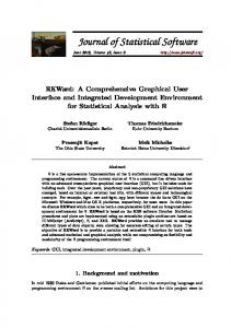
2.1. Mesh construction The basic tools for building basis function representations are provided by the low level function inla.mesh.create() and the three high level functions inla.nonconvex.hull(loc, ...), inla.mesh.2d() and inla.mesh.1d(). The latter function defines B-spline basis representations in one dimension (see Section 3.1 for an example). The remainder of this section gives a brief introduction to mesh generation for two-dimensional domains. The aim is to create the triangulated mesh on top of which the SPDE/GMRF representation is to be built. The example in Figure 1 illustrates a common usage case, which is to have semirandomly scattered observation locations in a region of space such that there is no physical boundary, just a limited observation region. When dealing with only covariances between data points, this distinction is often unimportant, but here it becomes a possibly vital part of the model, since the SPDE will exhibit boundary effects. In the R-INLA implementation, Neumann boundaries are used, which increases the variance near the boundary. If we intend to model a stationary field across the entire domain of observations, we must therefore extend the model domain far enough so that the boundary effects don’t influence the observations. However, note that the reverse is also true: if there is a physical boundary, the boundary effects may actually be desirable. The function inla.mesh.2d() allows us to create a mesh with small triangles in the domain of interest, and use larger triangles in the extension used to avoid boundary effects. This minimises the extra computational work needed due to the extension. R> m points mesh bnd mesh mesh loc.cartesian = inla.mesh.map(loc.longlat, projection = "longlat") R> mesh2 = inla.mesh.2d(loc = loc.cartesian, ...) Alternatively, a semi-regular mesh can be constructed using the more low-level command R> mesh2 = inla.mesh.create(globe = 10) where the globe parameter specified the number of sub-segments to use, when subdividing an icosahedron. The points are adjusted to lie on constant latitude circles. See Figure 3 for an example of how to plot fields defined on spherical meshes.
2.2. Mapping between meshes and continuous space One of the most important features is the inla.spde.make.A() functions, which computes the sparse weight matrices needed to map between the internal representation of weights for basis functions and the values of the resulting functions and fields. The basic syntax is
Journal of Statistical Software
11
● ●●
● ●
●
● ●
●●●
● ● ● ●● ●
● ● ●
● ●
● ● ●
● ●
●
● ●
● ● ● ●
● ● ●
●
● ●
● ● ●
●
● ●
●
● ●
●
●
●
● ●
● ●
●
●
●
●
● ●
●
● ●●
● ● ●● ● ●
●
●
●
●
●
● ●
●
●
●
●
●
●
●
●
● ●● ●
●
●
●
●
● ●
●
● ●
(a) Basic extended mesh
(b) Non-convex domain
(c) Non-convex mesh
(d) Extended non-convex mesh
Figure 1: Illustrations of meshes constructed based on a common set of domain definition points but different mesh generation parameters.
R> A spde R> R> R> R> R> + +
sigma0 mesh2 proj2a proj2b stack stack A x covariate y mesh.index st.est st.pred stack formula inla.result result plot(result[["marginals.range.nominal"]][[1]], type = "l", + main = "Nominal range, posterior density") The posterior means and standard deviations for the latent fields can be extracted and plotted as follows, where inla.stack.index() provides the necessary mappings between the inla() output and the original data stack specifications:
R> R> R> R> + R> +
index R> + R> R> R> + +
A
time R> R> R>
knots + +
stack1